HAL Id: hal-00565025
https://hal.archives-ouvertes.fr/hal-00565025
Submitted on 10 Feb 2011HAL is a multi-disciplinary open access
archive for the deposit and dissemination of sci-entific research documents, whether they are pub-lished or not. The documents may come from teaching and research institutions in France or
L’archive ouverte pluridisciplinaire HAL, est destinée au dépôt et à la diffusion de documents scientifiques de niveau recherche, publiés ou non, émanant des établissements d’enseignement et de recherche français ou étrangers, des laboratoires
A statistical-reaction-diffusion approach for analyzing
expansion processes
Lionel Roques, Samuel Soubeyrand, Jérôme Rousselet
To cite this version:
Lionel Roques, Samuel Soubeyrand, Jérôme Rousselet. A statistical-reaction-diffusion approach for analyzing expansion processes. Journal of Theoretical Biology, Elsevier, 2011, 274 (1), pp.43-51. �10.1016/j.jtbi.2011.01.006�. �hal-00565025�
A statistical-reaction-diffusion approach for analyzing expansion processes
Lionel Roquesa,∗, Samuel Soubeyranda, J´erˆome Rousseletb
aUR 546 Biostatistics and Spatial Processes, INRA, F-84000 Avignon, France bUR 633 Zoologie Foresti`ere, INRA, F-45166 Ardon Olivet, France
Abstract
In this article, we propose a method for analyzing the spatial variations in the range expansion of the pine processionary moth (PPM), an invasive species in France. Based on binary measurements – the presence or absence of PPM nests – the proposed method allows us to infer the local effect of the environment on PPM population expansion. This effect is estimated at each position x using a parameter F (x) that corresponds to the local PPM fitness. The data type and the two stage PPM life cycle make estimating this parameter difficult. To overcome these difficulties we adopt a mechanistic-statistical approach that combines a statistical model for the observation process with a hierarchical, reaction-diffusion based mechanistic model for the expansion process. Bayesian inference of the parameter F (x) reveals that PPM fitness is spatially heterogeneous and highlights the existence of large regions associated with lower fitness. The factors underlying this lower fitness are yet to be determined.
Keywords: mechanistic-statistical model, reaction-diffusion, pine processionary moth, Bayesian
inference, species range
1. Introduction
Recent experimental studies have reported a northward geographic range expansion of the pine processionary moth (Thaumetopoea pityocampa, Lepidoptera: Notodontidae, abbreviated as PPM below). In the Paris Basin, France, its range has shifted 87 km northward between 1972 and 2004, with a notable acceleration (55 km) during the last 10 years (Battisti et al., 2005; Robinet et al., 2007). Since the winter of 2005 − 2006, this expansion has been especially well documented with the establishment of a GPS-referenced map of the front winter nests all over France.
Because of its impact on forests, this expansion is likely to have important ecological conse-quences. It may also cause sanitary issues. The PPMs are entering semi-urban and urban areas; therefore, the insect has progressed from mere forest pest to urban medical threat. The threat arises from the way these organisms protect themselves against predation. When threatened, mature lar-vae release irritant hairs that cause allergic reactions in both man and warm-blooded domestic animals; reactions range from the cutaneous type to anaphylactic shock (Doutre, 2005). The con-tact of this type of insect with human and domestic animal populations that are not physiologically or behaviorally accustomed to it is likely to generate serious medical and veterinary threats in the near future.
Extensive measurements that have been carried out at different spatial scales in France show that the northern range of the PPM is far from flat. This indicates that population expansion
∗Corresponding author
is faster in some regions. Determining these regions is of crucial importance for controlling and preventing PPM expansion. In this study, we focus on a site located in the Paris Basin. Our goal is to build a map that describes the environment in terms of its local effect – whether it be favorable or unfavorable – on PPM expansion.
Our approach uses a model with a main parameter that measures the local PPM fitness at each spatial position. Like many other models in ecology this parameter results from the intertwined effects of several factors and cannot be directly measured. However, it can be estimated using observations of the population dynamics of interest (Klein et al., 2008; Soubeyrand et al., 2009a,b); here, we use observations of the position of PPM nests at the study sites.
The construction of a PPM expansion model that enables parameter estimation raises two non-classical difficulties: 1) the type of data we are dealing with – binary and incomplete observations of the presence of PPM nests; and 2) the life cycle of the PPM – the nest density evolves through a discrete-time process, but this evolution results from the dispersal and laying of adult PPMs, a continuous-time process.
We propose a mechanistic-statistical approach (Berliner, 2003; Soubeyrand et al., 2009a,b; Wikle, 2003) that combines a statistical model for the observation process with a hierarchical, reaction-diffusion based mechanistic model for the expansion of PPM nests. The statistical model bridges the gap between continuous data (nest densities) and binary data (observations) and, con-versely, provides a way to estimate the parameters of the mechanistic model based on the observed data. With a mechanistic model we are able to describe the discrete-time evolution of nests as a function of continuous-time adult dispersal and of the environmental effect on PPM fitness.
The choice of a reaction-diffusion model for adult dispersal was guided by observing the spatial genetic structure of PPM, which indicates a diffusive dispersal at the country scale (Rousselet et al, unpublished data). Moreover, the numerical integration of reaction-diffusion models is generally very fast. In the context of parameter inference, where many simulations are required, this speed is a considerable advantage compared to other approaches, such as individual based models.
In this work, we adopt a Bayesian framework for estimating the effect of the environment on PPM expansion. This framework is particularly convenient for mechanistic-statistical models that contain a latent structure because it allows the estimation of the unknowns of the model and a direct assessment of the estimation uncertainty (see e.g. Berliner, 2003; Wikle, 2003).
2. Data
2.1. Life cycle of the PPM
The biological cycle of the PPM has been known since the 18th century (R´eaumur, 1736). A complete description of this cycle can be found in Huchon and Demolin (1970). We summarize only the main features here.
The life cycle of the PPM usually lasts for one year and can be divided into two main stages: 1) the ovo-larval stage and 2) the adult stage. Throughout this paper we take the convention that the life cycle starts at the beginning of the adult stage.
Adult stage: In the study area, the adult stage starts at the beginning of the summer when
adult moths emerge from the soil and begin taking flight. Next, mating and spreading occurs. Females lay 70-300 eggs, which are usually deposited simultaneously on host trees (Huchon and Demolin, 1970). Female life expectancy ν is about 1 day (Robinet, 2006), and the duration of the flight period of adult moths is about two months.
Ovo-larval stage: Caterpillars emerge from eggs during the second half of summer. Immediately
after emergence, they build a common silk nest around which they feed gregariously on pine foliage. The position of the nest changes but remains on the same tree, stabilizing only when cold weather
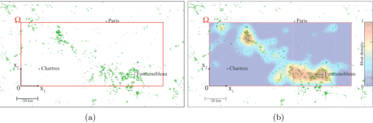
+ Paris 20 km + Chartres + Fontainebleau x 1 x 2 0 Ω (a) + Paris 20 km + Chartres + Fontainebleau x1 x2 0 Ho st de nsit y 0 1 Ω (b)
Figure 1: Location of the study site. The study site Ω is represented by a red rectangle. The coordinates of the corners of Ω are (N 48 18’ 22”,E 1 14’ 44”) for the bottom-left corner and (N 48 50’ 54”,E 3 3’ 32”) for the top-right corner. In Fig. (a), the study site is represented together with the positions of host trees (green regions). The smoothed host tree density in the study site is represented in Fig. (b).
arrives. At the beginning of spring, the caterpillars leave the nest and dig into the soil where they transform into pupae and remain for a few months until the next adult stage.
The clutch size, laying frequency and survival rates during the ovo-larval and adult stages may be influenced by environmental factors. Therefore, PPM fitness may depend on the spatial position of the individuals. In this paper we aim to estimate this local PPM fitness.
Remark 2.1. Unlike what happens in the endemic areas (Robinet, 2006), PPM populations do
not exhibit any temporal cycle outbreak in the newly colonized areas (A. Roques, unpublished data). Natural enemies have not followed the recent expansion of the PPM and quite a low rate of egg parasitism was observed in the study site (Imbert et al., in preparation).
2.2. Study site and binary measurements of the PPM range
The study site is a rectangular region Ω that is 134 km× 60 km, located in the Paris Basin (Fig. 1 (a)). This site contains urban, urban fringe, forest and agricultural areas. Preliminary large-scale observations by INRA URZF (UR633) have shown that, in 2005, PPM nests were present in the southern part of the study site (i.e. at some points (x1, x2) with x2 = 0) and were not present in its northern part (i.e. for x2= 60 km).
The PPM range has been measured during 2007, 2008 and 2009 (winters 2006-2007, 2007-2008 and 2008-2009) through direct observations of the presence of PPM nests. These measurements were conducted by INRA URZF. The study region was mapped into a lattice made of IΩ = 2010
square cells ωi of the same size 2 km × 2 km. For each year n a certain number JΩn of cells
were observed; however, observations were not exhaustive: Jn
Ω < IΩ. Moreover, only binary data
(presence or absence of PPM nests) have been recorded (Fig. 2 (a)-(c)). These data indicate a northward range expansion of the PPM, at an average speed of 4.2 km/year (4.1 km between 2007 and 2008 and 4.2 km between 2008 and 2009, see Fig. 2 (d))1.
2.3. Host trees
PPM host trees consist of several pine species. Potential host trees in the study region are essentially Pinus nigra and Pinus sylvestris. The positions of pine forests in the study site were
1During each year n, and at each longitude x
1where PPM nests have been detected, we can define the northernmost
latitude xn
2(x1) where PPM nests have been detected. The average expansion speed between years n − 1 and n
corresponds to the (possibly negative) distance xn
2(x1) − xn−12 (x1) averaged over all longitudes x1where PPM nests
+ Paris 20 km + Chartres + Fontainebleau x 1 x 2 0 Ω (a) 2007 + Paris 20 km + Chartres + Fontainebleau x 1 x 2 0 Ω (b) 2008 + Paris 20 km + Chartres + Fontainebleau x 1 x 2 0 Ω (c) 2009 20 km x 1 x 2 0 Ω 2009 2008 2007 (d)
Figure 2: (a), (b) and (c): Observation data. Blue squares in the study site Ω correspond to observed cells ωiwhere
PPM have not been detected. Red squares correspond to cells ωiwhere PPM nests have been detected. (d): Position
of the northernmost points where PPM nests have been detected during years 2007, 2008 and 2009.
available from the French National Forest Inventory database (Fig. 1 (a)). Whereas the existence of isolated trees between those forests is known, their exact positions were not available. To take these isolated trees into account host density was modeled by applying a Gaussian smoothing kernel on the forest position data (with average 0 and standard deviation 10 km) so that the tree density is never 0 over the study region. Tree density was then normalized so that its maximum value is 1 (Fig. 1 (b)).
3. Mechanistic-statistical model
The main objective of our model is to assess whether there are some regions in the study site that are more favorable to PPM expansion, and to determine the locations of these regions. The model that we propose combines a statistical model for the observation process with a hierarchical mechanistic model for the expansion of PPM nests. The PPM nest density at the end of the life cycle is represented as a function of the adult density during the whole adult stage and of environmental covariates. Adult density is modeled with a classical reaction-diffusion equation.
3.1. Statistical model for the observation process
The nature of the data forces us to use discrete space and time variables for the observation model. As explained in Section 2.2, the study site Ω was divided into IΩ square cells ωi of the
same area ρ = 4 km2. Discrete time is indexed by n = 0, . . . , N ; the interval between n and n + 1
corresponds to one year (=one cycle). We denote by Obsn(i) the binary variable that takes the
value 1 if PPM nests have been detected and 0 if no nest has been detected in the cell ωi at time
If a cell ωi has been observed during year n, the probability that Obsn(i) = 1 depends on the
local nest density in the cell ωi. We make the simplifying assumption that this probability only
depends on the average nest density Un(i) – expressed in nest units2 per unit area – in the cell ωi
at time n. Denoting by un(x) the local density of PPM nests at the end of the invasion cycle of
year n, we get: Un(i) = 1 ρ Z ωi un(x)dx. (3.1)
We assume that the detection variables are independently drawn from Bernoulli distributions con-ditionally on the average densities Un(i) through the following formula:
Obsn(i)|Un(i) ∼ Bernoulli{d(Un(i))}, (3.2)
i.e. Obsn(i) = 1 with probability d(Un(i)) and Obsn(i) = 0 with probability 1 − d(Un(i)). The
probability of successful detection thus depends nonlinearly on Un(i) through the function d.
As-suming that in each unit area each nest unit is independently detected with probability p, it follows that the function d is:
d(s) = 1 − (1 − p)ρ s. (3.3)
Note that (3.1) together with (3.3) imply that d(Un(i)) does not depend on ρ but simply on
the total nest units in ωi,Rω
iun(x)dx.
3.2. From continuous-time adult dispersal to discrete-time spread of nests
This section is devoted to the construction of a model that describes the evolution of PPM nest density. The model depends on a fitness parameter that summarizes the local effect of the environment on the emergence of PPM nests.
3.2.1. Nest density: a function of adult density and environmental factors
Because of the life cycle of PPM (see Section 2.1) the nest density evolves through a discrete-time process. However, this evolution results from the dispersal and laying of adult PPMs, which is a continuous-time process. Our aim here is to build a model which expresses nest density as a function of the adult density during the whole adult stage and of an environmental factor F (x). The mating processes are neglected in our model; thus, we only deal with female adult PPM density.
Let w∗(x, v
0,n) correspond to the cumulated (female) adult density at the position x at the end
of the adult stage, measured in time×individuals per unit area, starting from an initial density
v0,n. If f (x) measures the frequency of nest creation per individual in the absence of demographic constraints, the number w∗(x, v
0,n) × f (x) corresponds to the nest density which would be obtained
at the end of one cycle in the absence of constraints. Thus, the nest density un(x) at the end
of year n and at the position x can be computed by taking the minimum between this value
w∗(x, v
0,n) × f (x) and the local environmental capacity. Namely, we obtain:
un(x) = min (w∗(x, v0,n) f (x), Kχ(x)) , (3.4) where K is a carrying capacity (maximum PPM nest units per host unit) and χ(x) corresponds to host population density depicted in Fig. 1 (b). Without loss of generality, we can assume that the carrying capacity K is equal to one nest unit per host unit, which implies that K = 1.
2We choose to work with the number of nest units instead of the number of nests. Firstly, the number of nest
units need not be integers; this facilitates the formal setting of our method. Secondly, nest size can vary greatly and large nests are easily detected compared to smaller nests. It is therefore more natural to define the detection probability p with respect to a nest unit rather than a nest.
The nest density can be computed recursively by setting v0,n+1(x) = r(un(x))un(x), where
r(un) corresponds to the number of (female) adult individuals per nest unit. It is assumed here
that r(un) depends only on the local nest density (see Remark 2.1) through the formula:
r(un) = R1 + uun
n, (3.5)
for some R > 0. Formula (3.5) implies that the maximum number r = R of (female) adult individ-uals per nest unit is approached at high nest densities, whereas low densities lead to low values of
r. The function r thus takes an Allee effect into account (see Remark 3.2).
Assuming that the frequency of nest creation f and the host density χ do not depend on n and since w∗(x, v
0,n) depends linearly on v0,n(see the note below equation (3.11)), combining equations
(3.4) and (3.5), we obtain: un+1(x) = min ½ w∗ µ x, u 2 n 1 + un ¶ F (x), χ(x) ¾ , (3.6)
where F (x) = R f (x) measures the maximum number of (female) adults who might emerge during year n + 1 – in the absence of demographic constraint – for one (unit of adult density×unit of time) at the position x during year n. Thereafter, F (x) is called the local fitness at the position x; in this study we assume F (x) to be independent of n.
The equation (3.6) enables us to compute the nest density un(x) at each year n ≥ 1, given an
initial condition u0. We define u0 with equation (3.6), by setting, for each x = (x1, x2): u−1(x1, x2) = χ(x) e− min(0,2−x2)2.
Thus, u−1 corresponds to a virtual nest density in which hosts are considered saturated for x2 <
2 km and nest density decreases exponentially quadratically for values of x2 greater than 2. This
definition of u−1 means that PPM nests were present at the southern range of the study site one
year before the first observation.
Remark 3.1. By “in the absence of demographic constraints” we mean that the frequency of nest
creation f (x) and the local fitness F (x) do not take the environmental carrying capacity into
ac-count. The carrying capacity is incorporated in the computation of the nest density un(x) through
the terms min (·, K χ(x)) and min (·, χ(x)) in equations (3.4) and (3.6), respectively. This allows us to focus on the environmental effects other than those of saturation, which is already believed to be positively correlated with local fitness.
Remark 3.2. The Allee effect occurs when the per capita growth rate reaches its maximum at a
strictly positive population density. At low densities, the per capita growth rate may then become negative (strong Allee effect). Allee effect is known in many species (Allee, 1938; Dennis, 1989; Veit and Lewis, 1996). Experiments show that PPM clutches which are on the same tree tend to regroup in a bigger nest (ANR project “URTICLIM”, unpublished data) and that mortality inside the nest is negatively correlated with nest size (P´erez-Contreras et al., 2003). Thus, the higher the PPM nest density, the bigger the nests and the higher the survival rates are.
3.2.2. A diffusion model for the cumulated adult density
We recall the simplest diffusion equation:
∂v
where D > 0 stands for the diffusion coefficient. Starting from an initial condition v(0, x) = v0(x) ≥
0 corresponding to the initial (female) adult density at the beginning of the cycle3, the solution
v(t, x) of (3.7) describes the expected (female) adult density at time t and position x, assuming
that the individuals move according to uncorrelated random walks with constant move length in an open environment (see e.g. Okubo and Levin, 2002; Turchin, 1998). Here we assume that Ω∗ is a rectangle (0, 134) × (0, 120) which extends Ω in the northern direction. No-flux conditions are imposed at the boundaries {x1 = 0}, {x1 = 134} and {x2 = 0} meaning that as much individuals
exit the domain as individuals enter the domain at these boundaries. Absorbing conditions are imposed at the boundary {x2= 120}. In other terms:
∂v ∂x1 (t, 0, x2) = ∂v ∂x1 (t, 134, x2) = ∂v ∂x2 (t, x1, 0) = 0 and v(t, x1, 120) = 0. (3.8) In addition to dispersal we have to consider that at each time unit a fraction 1/ν of the individuals die (ν is the life expectancy). Thus, we obtain the reaction-diffusion equation for the (female) adult density v : ∂v ∂t = D∆v − v ν, t > 0, x ∈ Ω ∗. (3.9)
The cumulated population density at time t and position x is defined by
w(t, x) =
Z t
0
v(s, x) ds. (3.10)
Integrating (3.9) between 0 and t we observe that w also satisfies a reaction-diffusion equation:
∂w
∂t = D∆w − w
ν + v0(x) for t > 0 and w(0, x) = 0, x ∈ Ω
∗. (3.11)
Note that w depends linearly on v0; if ˜w satisfies ∂ ˜w/∂t = D∆ ˜w− ˜w/ν +κv0(x) for some κ > 0, with
˜
w(0, x) = 0 and the same boundary conditions as w and v, then ˜w/κ satisfies the same equation
as w. By uniqueness of the solution of this equation we get ˜w/κ = w and therefore ˜w = κw.
The cumulated adult density at the end of the adult stage is defined at each position x ∈ Ω ⊂ Ω∗ by:
w∗(x) = w(t∗, x), (3.12)
where t∗ is such that a random individual born at t = 0 has a probability smaller than 0.01 to be
still alive at t = t∗. In our computations we have used t∗= ν ln(100) = 4.6 days (see Appendix A).
4. Statistical inference
In this section, we estimate the local fitness parameter F (x) and the diffusion parameter D of the mechanistic-statistical model presented in Section 3 based on the observations of Section 2.2.
3The emergence period of adult PPMs stretches over two months (see Section 2.1). However, if we neglect the
interactions between individuals during the adult stage then it can be assumed in our computations (without loss of generality) that the emergence of all adults occurs simultaneously at the beginning of the adult stage.
4.1. Likelihood function
Let (nk)k=0,...,N correspond to observation years. We denote by Obs =©Obsnk(i), i = 1, . . . , J
nk
Ω , k = 0, . . . , N
ª
the set of all the observations and by U = {unk(x), k = 0, . . . , N } the set of nest densities during
the years (nk)k=0,...,N.
If the densities unk are governed by the model presented in Section 3.2, the set U depends deterministically on the unknown parameters F and D. The other parameters in the model being given, the set U is completely determined by F and D. Thus the conditional distribution of the observation process verifies:
P (Obs|U) = P (Obs|F, D) = L(F, D), (4.13)
where L(F, D) stands for the likelihood of the set of parameters {F, D}. Because, for k = 0, . . . , N, the sets of observations Obsnk =
© Obsnk(i), i = 1, . . . , J nk Ω ª during year nk and conditionally on unk are independent from each other, we have:
P (Obs|U) =
N
Y
k=0
P (Obsnk|unk).
Additionally, by assumption (see Section 3.1), for each k ∈ [0, N ] and for i = 1, . . . , Jnk
Ω the
observation variables Obsnk(i) depend on unk only through the average nest density Unk(i) in the cell ωi. Moreover, the variables Obsnk(i), conditionally on Unk(i), are also independent. We
therefore have: P (Obs|U) = N Y k=0 JYΩnk i=1
P (Obsnk(i)|Unk(i)). (4.14)
Using formulas (3.2), (4.13) and (4.14), we obtain:
L(F, D) = N Y k=0 JYΩnk i=1
[Obsnk(i)d(Unk(i)) + (1 − Obsnk(i))(1 − d(Unk(i)))] .
For our computations we took p = 0.9 in the definition of the function d (see eq. (3.3) and Appendix B).
4.2. Bayesian estimation of the parameters
In our computations, the study site Ω is discretized into NF rectangular subcells of the same
size, and F (x) is assumed to be constant equal to a value Fi on each cell i, for i = 1 . . . NF.
Besides, it is assumed that F is constant in Ω∗ \ Ω : F (x) = F
NF+1 for all x = (x1, x2) such
that x2 ∈ [60, 120). Thus estimating F becomes equivalent to estimating the parameters Fi for
i = 1, . . . , NF + 1.
Prior parameter distribution
In the absence of further information we assume independent uniform prior distributions in [0, F max] of the parameters Fi, and a uniform prior distribution (independent of F ) in [0, Dmax]
of the parameter D :
1st quartile 3rd quartile median 0 x1 x2 0 x1 x2 0 x1 x2 0 150
Figure 3: First, second (median) and third quartiles of the posterior distribution of the fitness parameter F in the domain Ω.
From the definition of F (x), and because each female can bear at most 300 eggs with a sex-ratio close to 1 : 1, we fixed F max = 150. The value of Dmax was set to4 30km2/day.
Posterior inference
The posterior distribution of the parameters is obtained using Bayes theorem:
P (F, D|Obs) ∝ L(F, D) π(F, D).
The posterior inference is performed by constructing a Markov chain, with a stationary distribu-tion that matches the posterior distribudistribu-tion, by using a classical Metropolis-Hastings algorithm (Hastings, 1970; Metropolis et al., 1953) that is detailed in Appendix C.
4.3. Results
Posterior distribution of the fitness parameter F
The first, second (median) and third quartiles of the posterior distribution of the fitness param-eter F are presented in Fig. 3. The distribution of F is clearly different from the prior distribution. This indicates that the observation data really do carry information about the distribution of F.
We can also observe that the distribution of the fitness F is spatially heterogeneous: the poste-rior distribution of Fi strongly depends on the position of the cell i. In particular, there are several
large unfavorable regions (black regions in Fig. 3).
Besides, the distribution of F is spatially structured in the sense that close regions tend to resemble each other. This can be assessed rigorously by using a permutation test (Manly, 1997). At each position i ∈ {1, NF}, we can compute the mean Kolomogorov-Smirnov distance between
the distribution of F at the position i and the distribution of F in the neighboring cells. Averaging this distance over all positions, we get a measure H of the similarity between the distributions of
F in neighboring cells. Considering any permutation σ of {1, NF}, we can compute a measure Hσ
of similarity between neighboring cells in the permuted coordinates (see Appendix D for a detailed
4When the diffusion coefficient is equal to D, the average dispersal distance of the individuals after τ days is
L =√π τ D km. Whenever τ = 1 (i.e. the life expectancy) we have for a low value of D L(τ = 1, D = 10−3) = 0.06 km
0 2 4 6 8 10 12 0 0.05 0.1 0.15 0.2 0.25 D Probability density
Figure 4: Posterior distribution of the diffusion parameter D.
computation of H and Hσ). Thus we can test the null hypothesis of unrelatedness between the
posterior distributions of F in neighboring cells by assessing if H is significantly low given the distribution of Hσ. The p-value of this test is the proportion of values of Hσ obtained for 104
random permutations σ that are lower than H. The obtained p-value is lower than 10−4. This
shows the similarity between posterior distributions of F in neighboring cells, i.e. the existence of a spatial structure in the posterior distribution of F.
Note that the posterior distribution of F does not seem to be strongly correlated with the host density χ(x) (Fig. 1 (b)). This is a consequence of our definition of the local fitness, which is computed “in the absence of demographic constraints” and therefore does not take the environ-mental carrying capacity into account (see Remark 3.1). Thanks to this definition, the posterior distribution of F contains more information than the mere host density map. Still, host density can have an effect on F (x) among other covariates. However, the lack of resemblance between the maps in Fig. 3 and the host density χ(x) indicates that this effect is relatively small.
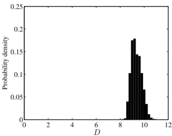
Posterior distribution of the diffusion parameter D
The posterior distribution of the diffusion parameter D is clearly different from the prior dis-tribution (Fig. 4). The posterior median of D is equal to 9.3 (mean 9.4 and standard error 0.4). This value D = 9.3 corresponds to an average dispersal distance equal to √πτ D = 5.4 km when τ = 1 (i.e. the life expectancy). This is higher than usually observed for Lepidoptera (see Kareiva
(1983) and Shigesada and Kawasaki (1997), page 55) and may indicate that the dispersal is not purely diffusive.
Model fit
Our model leads to a significantly better fit than a model without diffusion (i.e. when D = 0.). This can be assessed by computing the modal value of the posterior log-likelihood. We obtain respectively −10086 for the model without diffusion and −676 for the full model. This is a strong evidence against the model without diffusion. It is confirmed by the Deviance Information Criterion (DIC, see Spiegelhalter et al. (2002)), a Bayesian method of model comparison which is based on the posterior mean of the log-likelihood, which is higher in the case without diffusion (DICD=0= 20174) than in the full model (DICD = 1430).
Our model allows us to reconstruct the average nest densities Un corresponding to the modal
values of the parameters F, D. These densities are depicted in Fig. 5 together with the northernmost points where PPM nests have been detected, for each year of observation.
x 1 x 2 0 134 km 60 km (a) 2009 x 1 x 2 0 134 km 60 km (b) 2008 x 1 x 2 0 134 km 60 km (c) 2007 0 1 Nest density
Figure 5: Average nest densities Uncomputed for the modal values of the parameters F, D, in the domain Ω, together
with the northernmost points where PPM nests have been detected during years 2007, 2008 and 2009. Yellow areas correspond to 95% confidence intervals for the northernmost points of detection.
At first glance, it appears that the northward expansion of the PPM nest density matches well with the progression of the northernmost points of detection. To assess the goodness of fit of the model, we computed 95% confidence intervals for the northernmost points where PPM nests can be detected in the observation regions. The confidence intervals have been computed by simulating 1000 times the observation process on the nest density maps Un corresponding to the modal values
of the parameters F, D. These intervals are indicated by yellow areas in Fig. 5. We observe that most of the northernmost points of detection fall within the confidence intervals (97% of them are included in the confidence intervals).
It can be noted that since the carrying capacity has been fixed to one nest unit per host unit, the nest densities Un are lower than the host density χ(x). In particular, the nest densities are
small in the southwest corner of the study site. Note also that our model predicts the existence of some PPM nests beyond the 2009 observation region.
5. Discussion
On the basis of the binary observations of PPM nest ranges, we were able to describe the environment in terms of its effect on PPM expansion. To achieve such results, we dealt with several technical difficulties related to the type of data and to the life-cycle of the PPM.
To overcome these difficulties, we coupled a statistical model for the observation process with a hierarchical, reaction-diffusion based model for the expansion of PPM nests. This approach enabled us to compute the likelihood, at each position x of our study site, of a local fitness parameter F (x) that summarizes the effect of the environment on the emergence of new PPMs. More precisely, this parameter F (x) measures the number of PPM adults who might emerge during year n + 1 for one unit of adult density present at the position x during one unit of time in the course of year n. Variations in the parameter F (x) can therefore reflect local variations in either egg production, egg deposition rate, or in ovo-larval mortality rate. Thus the higher this parameter, the more favorable the environment is.
Using uniform prior distributions for the fitness parameter F (x) and for a diffusion parameter D, we performed a Bayesian inference of the posterior distribution P (F, D|Obs) given the observations. A comparison of the first, second and third quartiles of the distribution of F and an analysis of the distribution of D revealed that these distributions are clearly not uniform. Thus, the observations do carry some information on the distribution of the fitness and diffusion parameters.
Additionally, important gaps were observed between the fitness distributions at different loca-tions x in the study site. This shows the heterogeneous character of the environmental fitness: there are some regions in the study site which are more favorable than other regions. Interestingly, favorable and less favorable regions seem to be organized in clusters. This was confirmed by a rig-orous statistical analysis that shows that the distribution of F (x) varies smoothly with the location
x.
The median value of the posterior distribution of D is higher than usually observed for Lep-idoptera. This may indicate that the dispersal is not purely diffusive, i.e. that long-distance dispersal events may occur. This hypothesis is also supported by recent experimental data (Robi-net et al., preprint). Such a high diffusion coefficient would lead to a high speed of range expansion in a homogeneous favorable environment. However, our study shows that the environment is not homogeneous and the actual speed of range expansion (see Section 2.2) could be mainly limited by the presence of unfavorable regions (i.e. associated with low values of F (x)) such as the black regions in Fig. 3.
On the basis of these results, we plan to classify several covariates according to their effect on PPM expansion. The function F (x) can be seen as the superposition of the effects of several covariates. Covariates that are believed to play an important role on PPM expansion are, for example, the type of host trees (Huchon and Demolin, 1970), the presence of trees other than host trees, the presence of urban areas and the mean winter temperatures (Battisti et al., 2005). Note that interannual environmental variations are not taken into account in our model. Such variation can however be incorporated in our model by allowing the fitness F (x) to depend on the time variable n.
The method that we have developed here can be adapted to several other situations. The use of a statistical model for the observation process permits jumping from one type of data (as given by the model of the underlying process) to another (as given by the observations). Consequently, it allows the computation of a likelihood function for the parameters of the model given the data. The hierarchical, reaction-diffusion based approach can also be adapted to the modeling of other types of impacts caused by biological pests. The main idea is to model the observable impact (here, the presence of nests) as a function of the pest density, integrated over the whole period where
pests are active (here, the adult stage).
Additionally, the reaction-diffusion model can be replaced by other types of models such as individual based models (Gross et al., 1992; Kareiva and Shigesada, 1983; Marsh and Jones, 1988) or integral models (Hamel et al., 2010; Kawasaki and Shigesada, 2007; Kot et al., 1996). The method proposed in Section 3.2.1 for modeling the nest density as a function of adult density and environmental factors is independent of the underlying model for adult dispersal. However, as al-ready emphasized, the choice of the reaction-diffusion approach was encouraged by computational speed advantages and by an observation of the spatial genetic structure of the PPM. It is also note-worthy that reaction-diffusion models are in good agreement with the dispersal properties of some species, at least qualitatively (Murray, 2002; Okubo and Levin, 2002; Shigesada and Kawasaki, 1997; Turchin, 1998); these models can describe constant speed as well as accelerating range ex-pansions (Hamel and Roques, 2010; Roques et al., 2010). Furthermore, recent developments in the field of inverse problems show that most parameters of reaction-diffusion models can be de-termined using only spatially-incomplete measurements of the population density (Cristofol and Roques, 2008; Roques and Cristofol, 2010). Although the measurements in these papers are not of the binary type, nor are they blurred by an observation uncertainty, such a one-to-one and onto relationship between partial measurements of the population density and parameters of the model suggests that reaction-diffusion is a good framework for estimating the effects of environmental covariates.
In our reaction-diffusion model for adult dispersal (3.9) the diffusion coefficient was assumed to be constant. Non-constant diffusion operators could have been used instead of D∆v, e.g. ∆(D(x)v) (see Roques et al. (2008)), and local diffusivity D(x) could have been estimated together with
F (x). However, as in classical Fisher-KPP reaction-diffusion models in homogeneous environments
(Fisher, 1937; Kolmogorov et al., 1937) where diffusion and growth have an identical effect on the rate of expansion, D(x) and F (x) could have close effects, leading to an identifiability problem. Estimation of the parameters would also require a lengthy numerical resolution of the diffusion model, all the more time-consuming as the diffusion operator is not constant.
Appendix A: Computation of the cumulated density w∗
The solution w of (3.11) was computed using Comsol Multiphysicsr time-dependent solver,
using second order finite element method (FEM). This solver uses a method of lines approach incorporating variable order variable stepsize backward differentiation formulas. Then w∗(x) =
w(t∗, x), where t∗ is computed as described below.
Denote by V (t) the total population at time t:
V (t) =
Z
Ω∗v(t, x)dx.
A value of t∗ such that V (t∗) ≤ V (0)/100 can be computed explicitly. Integrating the equation
(3.9) over Ω∗ and using Green’s formula we get:
V0(t) = Z
∂Ω∗∇v · n dS − V /ν,
where ∂Ω∗ corresponds to the boundary of Ω∗, n is the outward unit normal to ∂Ω∗ and dS is
a surface element. The boundary conditions (3.8), together with the positivity of v in Ω∗ (which follows from the parabolic maximum principle, see Protter and Weinberger (1967)) then imply
Thus V satisfies V0(t) ≤ −V /ν and V (t) ≤ V (0)e−t
ν. Taking t∗ = ν ln(100) we get V (t∗) ≤
V (0)/100.
Appendix B: Estimation of the nest detection probability
The probability p of detecting one nest unit in a given unit area (see Section 3.1) was estimated on the basis of an additional data set: during the winter of 2008 − 2009, every tree was observed and the average PPM nest density U (i) was estimated in 100 previously observed cells ωi (say for
i = ik, with k = 1 . . . 100). This enables us to compute the likelihood of p for each p ∈ (0, 1) :
L(p) = P (Obs(ik)k=1...100|U (ik)k=1...100, p)
=Q100k=1[Obs(ik)dp(U (ik)) + (1 − Obs(ik))(1 − dp(U (ik)))] ,
where, as in (3.3), dp(s) = 1 − (1 − p)ρ s and ρ = 4 km2. A maximization of this likelihood function
permits us to estimate p ' 0.9.
The formula (3.3) for the probability d(s) of successful nest detection in a cell ω with average nest density s directly follows from the definition of the parameter p. Given the area ρ of ω, the number of nest units in ω is equal to s × ρ. Since we assume that each nest unit is independently not detected with probability (1 − p), the probability of not detecting PPM nests in the cell ω is (1 − p)ρ s. Finally, the probability of successful detection d(s), given the average density s is
therefore equal to 1 − (1 − p)ρ s.
Appendix C: Metropolis-Hastings algorithm
A Metropolis-Hastings algorithm was used to construct a Markov chain whose stationary dis-tribution is the posterior disdis-tribution P (F, D|Obs) of Section 4.2. This is an iterative rejection-sampling algorithm with steps that are detailed below:
Start at k = 0 : initialize F0= (F0
j)j=1...NF+1, D0.
while k ≤ Nh
• Draw q indexes {j1, . . . , jq} with a uniform law in [1, NF + 1].
• Draw q values ˆFj1, . . . , ˆFjq from a distribution Q( ˆFj1|Fjk1) × . . . × Q( ˆFjq|F
k jq).
• Draw ˆD from a distribution QD( ˆD|Dk).
• Set ˆFj = Fjk for j ∈ [1, NF + 1] \ {j1, . . . , jq}.
• Choose randomly with an uniform law ζ ∈ (0, 1).
• Compute δ = L( ˆF , ˆD) π( ˆF , ˆD) QD(D k| ˆD)Qq i=1Q(Fjki| ˆFji) L(Fk, Dk) π(Fk, Dk) QD( ˆD|Dk)Qq i=1Q( ˆFji|Fjki) .
• If ζ < δ, Fk+1 = ˆF and Dk+1= ˆD else Fk+1= Fk and Dk+1= Dk.
endwhile
We use the following distribution for the proposals ˆF and ˆD : for any parameter value Y we
assume that Q(X|Y ) (resp. QD(X|Y )) follows a gamma distribution with scale parameter λ > 0
(resp. λD) and shape parameter Y /λ (resp. Y /λD):
Q(X|Y ) ∼ Γ(λ, Y /λ) and QD(X|Y ) ∼ Γ(λD, Y /λD).
For our computations, we used λ = 0.5, λD = 0.1 and Nh = 105.
Appendix D: Computation H and Hσ
Recall that in Section 4.2 the study site Ω was discretized into NF rectangular subcells of the
same size, and F (x) was assumed to be constant equal to a value Fi on each cell i, for i = 1 . . . NF.
To each cell i we associate a neighborhood Vi (we use a 4-neighborhood system: j ∈ Vi if and only if the cells j and i have a common side). For each couple of positions i, j ∈ {1, NF}, we define
hi,j as the Kolomogorov-Smirnov distance between the distributions of Fi and Fj. Then, the mean
Kolomogorov-Smirnov distance between the distribution of F in the cell i and the distribution of
F in the neighboring cells is hi = Card(V1
i)
X
j∈Vi
hi,j, where Card(Vi) corresponds to the number of
neighbors of the cell i. Averaging over all cells, we define:
H = 1 NF NF X i=1 hi. (5.15)
Again, for any permutation σ of {1, NF} we can define:
Hσ = N1 F NF X i=1 hσi. (5.16) Acknowledgements
The authors are supported by the French “Agence Nationale de la Recherche” within the project URTICLIM and EMILE. They would like to thank the reviewers for their valuable suggestions and comments.
References
Allee, W.C., 1938. The social life of animals. Norton, New York.
Battisti, A., Stastny, M., Netherer, S., Robinet, C., Schopf, A., Roques, A., Larsson, S., 2005. Expansion of geographic range in the pine processionary moth caused by increased winter tem-peratures. Ecological Applications 15, 2084–2096.
Berliner, L.M., 2003. Physical-statistical modeling in geophysics. Journal of Geophysical Research 108, 8776.
Cristofol, M., Roques, L., 2008. Biological invasions: Deriving the regions at risk from partial measurements. Mathematical Biosciences 215, 158–166.
Dennis, B., 1989. Allee effects: population growth, critical density, and the chance of extinction. Natural Resource Modeling 3, 481–538.
Doutre, M.S., 2005. Occupational contact urticaria and protein contact dermatitis. European journal of dermatology 15, 419–424.
Fisher, R.A., 1937. The wave of advance of advantageous genes. Annals of Eugenics 7, 335–369. Gross, L.J., Rose, K.A., Rykiel, E.J., Van Winkle, W., Werner, E.E., 1992. Individual-based
modeling. Chapman and Hall, New York. pp. 511–552.
Hamel, F., Fayard, J., Roques, L., 2010. Spreading speeds in slowly oscillating environments. Bulletin of Mathematical Biology 72, 1166–1191.
Hamel, F., Roques, L., 2010. Fast propagation for KPP equations with slowly decaying initial conditions. Journal of Differential Equations 249, 1726–1745.
Hastings, W.K., 1970. Monte Carlo sampling methods using Markov Chains and their applications. Biometrika 57, 97–109.
Huchon, H., Demolin, G., 1970. La bio´ecologie de la processionnaire du pin. Dispersion potentielle - Dispersion actuelle. Revue Foresti`ere Fran¸caise Num´ero sp´ecial “La lutte biologique en forˆet”, 220–234.
Kareiva, P.M., 1983. Local movement in herbivorous insects: Applying a passive diffusion model to mark-recapture field experiments. Oecologia 57: 322-327. Oecologia 57, 322–327.
Kareiva, P.M., Shigesada, N., 1983. Analyzing insect movement as a correlated random-walk. Oecologia 56, 234–238.
Kawasaki, K., Shigesada, N., 2007. An integrodifference model for biological invasions in a pe-riodically fragmented environment. Japan Journal of Industrial and Applied Mathematics 24, 3–15.
Klein, E.K., Desassis, N., Oddou-Muratorio, S., 2008. Pollen flow in the wildservice tree, Sorbus torminalis (L.) Crantz. Whole inter-individual variance of male fecundity estimated jointly with dispersal kernel. Molecular Ecology 17, 33233336.
Kolmogorov, A.N., Petrovsky, I.G., Piskunov, N.S., 1937. ´Etude de l’´equation de la diffusion avec croissance de la quantit´e de mati`ere et son application `a un probl`eme biologique. Bulletin de l’Universit´e d’´Etat de Moscou, S´erie Internationale A 1, 1–26.
Kot, M., Lewis, M., van den Driessche, P., 1996. Dispersal data and the spread of invading organisms. Ecology 77, 2027–2042.
Manly, B.F.J., 1997. Randomization, Bootstrap and Monte Carlo Methods in Biology (2nd edn). Chapman and Hall, London.
Marsh, L.M., Jones, R.E., 1988. The form and consequences of random-walk movement models. Journal of Theoretical Biology 133, 113–131.
Metropolis, N., Rosenbluth, A.W., Rosenbluth, N.M., Teller, A.H., Teller, E., 1953. Equation of state calculations for fast computing machines. Journal of Chemical Physics 21, 1087–1092.
Murray, J.D., 2002. Mathematical Biology. Third Edition. Interdisciplinary Applied Mathematics 17, Springer-Verlag, New York.
Okubo, A., Levin, S.A., 2002. Diffusion and ecological problems – modern perspectives. Second edition, Springer-Verlag, New York.
P´erez-Contreras, T., Soler, J.J., Soler, M., 2003. Why do pine processionary caterpillars Thaume-topoea pityocampa (Lepidoptera, Thaumetopoeidae) live in large groups? An experimental study. Annales Zoologici Fennici 40, 505–515.
Protter, M.H., Weinberger, H.F., 1967. Maximum Principles in Differential Equations. Prentice-Hall, Englewood Cliffs, NJ.
R´eaumur, R.A.F., 1736. M´emoires pour servir l’histoire des insectes, Tome second. Imprimerie Poyale, Paris.
Robinet, C., 2006. Mathematical modelling of invasion processes in ecology : the pine processionary moth as a case study. PhD Thesis, CAMS, EHESS, Paris.
Robinet, C., Baier, P., Josef, P., Schopf, A., Roques, A., 2007. Modelling the effects of climate change on the potential feeding activity of thaumetopoea pityocampa (den. & schiff.) (lep., notodontidae) in france. Global Ecology and Biogeography 16, 460–471.
Roques, L., Auger-Rozenberg, M.A., Roques, A., 2008. Modelling the impact of an invasive insect via reaction-diffusion. Mathematical Biosciences 216, 47–55.
Roques, L., Cristofol, M., 2010. On the determination of the nonlinearity from localized measure-ments in a reaction-diffusion equation. Nonlinearity 23, 675–686.
Roques, L., Hamel, F., Fayard, J., Fady, B., Klein, E.K., 2010. Recolonisation by diffusion can generate increasing rates of spread. Theoretical Population Biology 77, 205–212.
Shigesada, N., Kawasaki, K., 1997. Biological invasions: theory and practice. Oxford Series in Ecology and Evolution, Oxford: Oxford University Press.
Soubeyrand, S., Laine, A.L., Hanski, I., Penttinen, A., 2009a. Spatio-temporal structure of host-pathogen interactions in a metapopulation. The American Naturalist 174, 308–320.
Soubeyrand, S., Neuvonen, S., Penttinen, A., 2009b. Mechanical-statistical modeling in ecology: from outbreak detections to pest dynamics. Bulletin of Mathematical Biology 71, 318–338. Spiegelhalter, D.J., Best, N.G., Carlin, B.P., van der Linde, A., 2002. Bayesian measures of model
complexity and fit. Journal of the Royal Statistical Society: Series B 64, 583–639.
Turchin, P., 1998. Quantitative analysis of movement: measuring and modeling population redis-tribution in animals and plants. Sinauer Associates, Sunderland, MA.
Veit, R.R., Lewis, M.A., 1996. Dispersal, population growth, and the Allee effect: dynamics of the house finch invasion of eastern North America. American Naturalist 148, 255–274.
Wikle, C.K., 2003. Hierarchical models in environmental science. International Statistical Review 71, 181–199.