Cavity resonators and wave guides containing periodic elements

lVADIATtOIN LAB-ORATO!-Rf M.I.T.

CAVITY RESONATORS AND WAVE GUIDES CONTAINING PERIODIC ELEMENTS

By

HERBERT GOLDSTEIN

B.S., College of the City of New York 1940

Se

APR

2

1946

SUBMITTED IN PARTIAL FULFILMET OF THE REQUIR&MES FOR THE DEGREE OF

DOCTOR OF PHILOSOPHY

FROM THE

MASSACHUSEPTS INSTITUTE OF TECHNOLOGY 1943

Signature of Author

Department of Physics, May 10, 1943

v A - AA

Signature of Professor

Charge of Research .. .. .,eu. :.v. .*.. Signature of Chairman of De artment

Section I Section II Section III Section IV Section V Appendix I Appendix II Appendix III

Resonant Modes of the Vane Magnetron... The Effect of End Zones ...

Experimental Study of a Linear Magnetron ...

1. Description of Apparatus ...

2. Discussion of Method and Results... 3. Measurement of Q ...

The Corrugated Wave Guide ...

1. Without End Zones ...

2. End Zones Present ...

The Corrugated Coaxial Line ... 1. Slots Enpty...

2. Slots Filled with Dielectric...

Tables of f and G

Measured Resonant Wave Lengths of a Linear Magnetron The Unloaded Q of a Linear Magnetron

SECRET

-SECRET

ACKNOWLEDGMENT

I wish to express my sincere gratitude to Professor I. C. Slater for having made this thesis possible, and for his

continued interest and encouragement. To the members of the Theoretical Group, especially Professors H. A. Bethe and N. H.

Frank, I am indebted for many suggestions and much helpful advice. Professor G. G. Harvey and Doctors H. Krutter and T. E. Lashof kindly supplied the experimental data for the corrugated wave

guides and coaxial lines. I also wish to thank Professor A. 1.

Heins and the Staff of the Computing Room under his supervision

I Resonant Modes of the Vane Magnetron

The resonant modes of vane type magnetrons are calculated, neglecting end effects and fringing near the vane edges. The effect of the cathode is con-sidered and found to be negligible for all except the lowest modes. Tables are presented which facilitate the computation of the resonant wave lengths over a

wide range of magnetron dimensions. The measured and computed values for three typical magnetrons differ by about 3%, presumably due to end effects. It is

shown in Section II that the fringing of the fields could not account for more than a 1% difference.

II Effect of End Zones

Several methods of calculating the end zone effect in a linear magne-tron are presented. In the first procedures appropriate tangential electric and

magnetic fields in the end zones are joined to the corresponding fields in the

oscillator cavities. These methods fail because the fields in the end zones

and the fields in the cavity which corresponds to the region between the cathode

and anode are not adequately matched. To improve this connection the currents

on the walls of this region are joined continuously to the currents in the end zone walls. The calculated end zone effect is then in qualitative agreement with experiment. The remaining discrepancy is probably due to the omission of damped modes which are important near the edges of the vanes.

Page 2

III Experimental Study of a Linear Magnetron

To investigate experimentally the effect of tne end zones a 10 slot linear magnetron cavity witn adjustable end plates has been constructed. Modes

in tne range from 6.5 to 12.5 cm. were detected and identified by means of the standing wave pattern picked up by a movable probe. The wave lengths of all the observed modes decrease as tne end zone is reduced. however for the higher modes

the decrease is slight, even at the smallest end zone used (.6 mm). Rough measure-ments of the unloaded Q were also made, and are approximately one half of the

com-puted values.

IV The Corrugated Wave Guide

The linear magnetron used as a wave guide is known as a corrugated wave guide. Formulas are derived for the guide wave length and attenuation. The com-puted wave l1nthls are within 5 of tho e r alues, but the attenuation is

about one fourth the actual value. It is shown that wave guides with relatively large end zones have the least attenuation.

V The Corrugated Coaxial Line

The corrugated coaxial line employs the same principle as the corrugated wave guide except that the slots are cut in the inner conductor. The wave length and attenuation in such a line are calculated both for empty slots and for slots filled with dielectric. Convenient approximate formulas for these quantities are presented which agree quite well with experiment. The attenuation due to losses in the dielectric is also considered.

SECRET

CAVITY RFBONATORS AND WAVE GUIDES CONTAINING PERIODIC ELBENTS

I. Resonant Modes of the Vane Magnetron

The resonant modes of slot and slot-and-hole magnetrons have been calculated by A. M. Clogston(l). This section presents similar

calculations for vane type magnetrons, i. e., in which the oscillator cavities are in the form of sectors of a cylinder.

An idealized type of vane magnetron will first be considered, a cross section of which is shown in Fig. 1. It is assumed long enough so that the end effects may be neglected. The cathode will also be omitted.

The space may be divided into two regions, the central cavity, I, and the individual oscillator cavities, II. In each region appropriate solutions of Maxwell's equations are used, obeying the boundary conditions on the metallic surfaces, which are considered ideal. Inside the oscil-lator cavities the radial component of the electric field will be neglected, that is, edge effects will not be taken into account.

The fields in each region are connected by requiring that the angular component of the electric field be continuous. The frequency at which the magnetron resonates is then determined by the condition that

the axial component of the magnetic field vary continuously from

Region I to II. Since the fields are only approximate, this condition cannot be fulfilled rigorously. One may however match the average magnetic field over the slot width.

(1)

3ECRET

Fig.

SECRET

SECRET

2 In the

jth

E .j

n r"

J,

(Mr)

N,()YrJ)

- N,

(Ur>

J,

(aY0

e

_-iw

,

5zj

aej

[J*

(

I,

-

N,

Nr

()

,

(r

)]e

)

cW =

C

X

where a is an arbitrary constant, n an integer, N the number of

oscillators. The phase factor e jIr is necessary in order that the fields have the same periodicity as the oscillators. The time dependence e

will be omitted in the following. The linear combinations of Bessel and

Neumann functions used above are cylinder functions and will be designated by C₁(k,r,r₂) and 01(k,r,r2 ) where:

C.,((K

r,f)

=IL

(

?)~(arJ

-

NV

()

Jm (r.)(

The fields may now be rewritten as:

E

ea

C,

(,r,r)J

Fej

3)

z)

In the central cavity, Region I, the appropriate solutions are standing waves. However traveling wave solutions may equally well be used, as the standing wave can always be obtained from the superposition of

waves traveling in opposite directions. The fields to be used are:

E

~

=P-T2'-b,

~

-Z

b

nte

(Jot

SECRET

3

There is also an Er component which is neglected.

The coefficients bm are determined by the conditions on E

at the boundary between the two regions. There are, at r = r ,

E

(r

E,3

(j)

where 24 is the angular width of an oscillator cavity. The Fourier coefficients b turn out as follows:

m

______

= -(IiPft

( I

55I "'V ~

-5)

)=O

The geometric series in Eq. (1-5) vanishes except when n- m=z t ,Ao,,2,--when it is equal to N. The coefficients thus become

b6 =K

- a

N,

M, C

,

e,)

I(I

-

6)

O othe w;se.

The average value of the magnetic field in I, averaged over the

slot width of the jth oscillator cavity is:

Lr=

Oli') IT

JS r(r) /

Equating this to the magnetic field in the oscillator cavity

following equation for the resonant frequencies:

f

n,

in

Y4

No

(0,

',

(

(I-'8)

c.,,T

U

-

7)

SECRET

4

The left hand side of the equation is periodic -in n with a period of

N/2. Thus the terms for n = n₁ are the same as those for n = n1 + N/2.

Since n must be integral, the number of modes is limited to N/2 (or if N is odd).

2

Actual magnetrons differ in several points from the idealized type considered here. The vanes are not wedges, but are rectangular

plates as shown in Fig. 2. The oscillator cavities may still be considered as very good approximations to sectors of a circle, but the center of the circle is now at 0' instead of 0. Then r1 and r2 in the oscillator fields are to be replaced by

/ _ d

Y2 tant

where 2d is the width of a vane. Eq. '(I-8) becomes

r

If the cathode is included in the calculation, the fields in Region I become so modified that the tangential electric field vanishes over the cathode surface. The fields are then:

-I,

0

(fr)Yr~(i

3

(I-

eo)

BJ-rh(fir)

kt(R

)

ri r,,'(r)

Jr

(e

r)

L'4'

NIr

) -

l',(MNr

) Jm(Il

r3)

(nr,){

-

V'(.Kr,

o

) J-X

L

r,,)

SECRET

/

/

/

/

/

/

/

Fig. 2

SECRET

/

/

r

SECRET

5 roots of the following equation:

'When m is large, .Tm'(kr) is small except near the vanes and the introduc-tion of the cathode will disturb the fields only slightly, and the resonant frequencies still less. Except for the lower modes the cathode has little effect, and therefore may be neglected in most cases.

For purposes of computation two functions f and G are defined by

C, (,r,'

)

/

and

si m )2

The function f can be considered as a function of x = k(r.' - r =

2 )=(r 2 - r

for different values of a parameter y = r₂'/r₁ '. For the range of x encountered in most magnetrons f is very nearly a linear function,

fz

a

li

(Y2 ~

r)

6(:

Appendix I gives tables of a and b for various values of y. G considered as a function of kr1 depends on the parameters N, n, and 05, and for n greater than 1 or 2 is quite accurately represented by a linear function

GM =.

o .

4r +

(3,

(1-15)

for the ranges involved. When n is 1 or 2, the representation is not

accurate, but may be used to give rough estimates. Tables of an and 0 are presented in Appendix I.

12)

(P-13)

SECRET

6

The resonant frequency is given by the root of

f

=G

-

(

(I-'

)

The resonant wave lengths of three magnetrons have been calcu-lated, neglecting the cathode, and are shown in Table I. For the first magnetron, which has a large cathode, the -wave lengths have also been

calculated including the cathode, using Eq. (I-11). The experimentally measured wave length, obtained from various sources, are also given in the table. Where two values are given for a mode, it indicates the mode

was split into a doublet due to the loops and probes inserted in the magnetron. It is seen that the effect of the cathode in the first tube is negligible for the n = 4 and higher modes. The cathode must have an even smaller effect in the other tubes. In almost all cases the experi-mental wave length is lower than the theoretical value. For the second

tube, the Westinghouse VA-1, part of this may be due to strap grooves near the extremity of the vanes. However the larger part of difference is the result of assuming the magnetron to be so long that the presence of the end zones may be neglected.

In the next section the effect of the finite length and end zones

SECRET

7

Table I

Resonant Modes of Three Vane Magnetrons

1. Model of the Columbia University Radiation Laboratory M-4 magnetron.

Scale factor = 7.55 ri = 1.728 cm. r2 - 3.26 cm. r3 = .957 cm. Anode length 4.18 cm.

#

2. Model of the Westinghouse VA-1 magnetron. Scale factor - 3.43

r = 1.73 cm. r2 -3.45 cm. r3 = .550 cm. Anode length = 3.36 cm. .0986 N = 18 X(Eq. 1-8') 11.92 cm. 10.80 10.38 10.05 9.96 9.84 9.78 X(exp.) 12.122 cm. 10.670 10.146, 10.115 9.857, 9.793 9.660, 9.633 9.557 9.480

U

+1.7%

SECRET

8

Table I (continued)

3. Magnetron described by Okress and Wang, P. 11, Radar Memo B-1,

Westinghouse Research Laboratories.

r = .68 cm. r2 w 1.950 cm. Anode length = .64 cm.

#

Operating Wave Length 8.05 cm.

n

SECRET

9 II. The Effect of End Zones

This section presents the results of several attempts to take into account the finite length of the oscillators and the cavities at

the ends.

To simplify the problem the circular magnetron is developed into a linear one, details of which are shown in Fig. 3. The linear magnetron may be continued indefinitely in the y-direction, in which case it will

act as a waveguide with a band of propagated wave lengths. On the other hand, it may be converted into a cavity by means of end plates in the xz plane. Such a linear magnetron will resonate only at a discrete set of frequencies determined by the requirement that the distance between the end plates be an integral number of half wave lengths in the y-direction. The modes will be labeled in accordance with the notation used for rec-tangular resonators. They will be designated by three indicesy, m, n giving the number of anti-nodes of the field in the x, y, and z directions respectively when the end cavities are reduced to zero. In all the following cases I = 0. Magnetrons operate in one of the (O,m,l) modes. The (O,m,2)

modes are characterized by a node in the z = 0 plane, and are generally of much higher frequency. They have been detected by Slater(2) and Tonks

and Crawford . The (0,m,3); (0, m, 4) etc., modes have still higher

frequencies.

The cavity may be considered as a special case of the linear magnetron used as a wave guide, for the effect of the end plates can be

T.

L. Tonks and S. N. Crawford, General Electric Research Laboratories,

rNaLI

z-z

-z-O

U

I

z

x

Zito

Section

d

-Y

'lizX

b

Plan

T

z

jAz

Elevation

Fig

3

=o

x;-SECRET

10 reproduced by an infinite set of images. The only distinction between the two is that the wave length in the y-direction in the cavity is limited to certain values.

The space will be divided into four regions as shown in Fig. 3a.

Regions III and IV constitute the end cavity or zone, Region II the

oscil-lator cavity, and Region I corresponds to the cavity between the cathode and anode. The fields in IV must be small and will not be considered explicitly. The method will be to set up appropriate solutions for the

fields in Regions I, II, and III and then connect or join them one to another.

The appropriate solutions in Region I are traveling waves propagated in the +y and -y directions. Since the wave number in the

y-direction, k , is always larger than the wave number, k, in empty space, the wave number in the x-direction must be imaginary. The relevant

compo-nents of the fields in I are

B

e

+00

E~

~

5ih

'C0c5I

-00 X

-00

with the condition

2. 2 2 2(f.)

and where k2-k Z has been designated by k ,s. The fields are transverse

z(4)

electric in the z-direction, i. e., EZ = 0. It has been shown by Slater (4

-- -

SECRET

11 that the periodicity of the fields in the oscillator cavities requires

the following relation between k and k

ym yo

/ti 'lo + --

M-r

(IT

Y

where Y is the distance between oscillators. From this Slater has also

shown that as the maximum value of k is s/Y, and the corresponding maximum wave length in the y-direction is 2Y. If the linear magnetron

is used as a waveguide k may take any value between 0 and x/Y. If

used as a cavity the possible values of k are , m -- ,2, . . . N;

where N is the number of oscillators contained in the length of the

cavity. The fields of Eq. (II-1) are suitable for that type of mode in

which the index n is odd. If the index n is even cos k z is replaced by sin kz, and sin k z by -cos k z.

Some of the components in the jth slot are:

:

b

io

_Cos

_{(X-Y-L) cos}

Mz

BH.

S

be

Cos

(')

+

Cosm

(-L)

cos,.

+

e

cos '"

,

x

-.

X -L)

cosh

IT

d

;r

coS

(11-i

t-

R

be

*

-

(

-)

N' (X-L) Cos

R,

SECRET

Y

The first term in each field corresponds to the principal mode; the second term contains the higher modes generated at the edges

of the slot at x = X, which decay exponentially in the interior of the

oscillator cavity. The third term likewise contains higher modes, due here to the edges at the top of the slot at z = z,.

The fields in I and II are connected by making some reasonable assumption as to the form of E across the slot at x = K. The coefficients

y

am, bm, and dm, which are essentially coefficients of a Fourier expansion, are then determined. The higher modes generated at the top edges are almost zero except for z close to + zl, and may therefore be neglected in performing this joining. Since the fields in I and II then depend in the same way on z, this z dependence will drop out. The joining is completed by requiring that the tangential magnetic field, averaged in some fashion, be continuous across the slot in the x = X plane. This requirement results in an equation connecting the wave numbers in the two regions. Examination of the fields shows that this relation may be written explicitly in terms of k and k I alone. That is, it will have the form

f

(X)

1

)

o0

_(1-

₆₎

SECRET

13 index) then k * is determined independently of the variation in the z-direction. The resonant frequency can then be found from

If the magnetron is of indefinite extent in the z-direction then k Z-O

and k=k x. Another limiting case occurs when Z=O, i. e., no end zones. The frequency is then given by

Y1

X

)_ '

(LITr-

7)

where n is the third index of the mode, and 2z the height of the oscillator cavities.

The particular expression to be used in Eq. (11-6) depends on the assumed form of the electric field across the slot. If the edge effects are completely neglected, and hence E is constant across the

y

slot, then Slater(5) has found that the relation is:

-

(

=

7

-

)

-x xx ray k ?IXYM K yd/a

The edge effects may be included to a high degree of

approxi-mation if one assumes the field which is calculated from the solution of the electrostatic problem. In treating the problem of a T-joint in a wave guide Frank and Chu(6) have suggested a field closely approximating the electrostatic solution which is of the following form:

AC

-

05 Z

C

Cos

The coefficients am, bm of Eqs. (II-1) and (11-4) are determined in terms of A and C. The average of the tangential magnetic field may then be

calculated in each region, and must join on at x=X. Similarly the averages

-- -

---T5)J.

14

with respect to the first Fourier component, sin , must be equal at

x - X. These two conditions result in two linear homogeneous equations for A and C. Eq. (11-6) is then given by the requirement that these equations have a non-vanishing solution.

The coefficients a must be such that E satisfies the boundary

m y

conditions on the walls and at the slots. These are

x ,, C sn x ~=0 - Y_$

d'~

dd

If both sides are multiplied by eikyn and integrated between (j

and (j + !)Y, the equation becomes:

iw~xa

e

S

in

h

A

+C

I-Cf

1 di

a(f

These integrals may be evaluated by changing the variable to 9 arc sin

+-2

SECRET

15 and using the expansion of e P sin 9 in Bessel functions .

expression is

1 2

Nw?

rd

The final

(L-

12)

-W

_6.d

_sin

|L

)

b

ba

0

₂

N

x' A

5ntllL

Y"

(/

d

,, s~in'rL

A

~C)

C0s

Y'

2

i

-

(

Here two cases must be distinguished. If m is odd,

T'

C2

C

A

bw

J

Yz.

XL

With these coefficients the z-component of the magnetic field in Region I is:

O X ) '- - ri C 2 XCaski Cosh

IT,

y

2

;E

Swh M-

X'

The average of this component across the jth slot is then

+W.2 _tQ1

)~

(]I1-1!5)

TJ.

and

bm -

^y'

*

>

(11 -13)

M

odd

(]

- m)

jo

ri "-j/

- i C

J, V%

cj/;z

sinh h X

I

SECRET

16

and the similar average, weighted by the Fourier component, sin ,

is given by Sh3 l

T r

d

(i-IL )

These are to be set equal to the corresponding averages of the field

in II, which are in fact

just

d

Y

A

t ax

L

cJ.(

X)

h,'xta-N,

-0-Imposing the condition that these two equations have non-vanishing solutions yields the desired relation between k and k ':

8

to"

nY

tav

h

hxY

)X,

-t

L

K%*

tanh

J-

I

-0

JO

J/

(.-17)

(TT

-

I

)

I

s;

4

x

1,

A

J

te

-

i C J,(hi

d)

tan

?Tx,3

kx

j Oj Y

A I (Ki

B (T) = -:1

_x

--

_Y

L" -lhe

C)4

N

j

Y

Y

S-~ U

SECRET

17

d

&

=4

_J/)

₊

U)

2)2r-8,4

For k large the cross terms S and 6 are small, vanishing identically when k = Hence the roots of Eq. (11-18) are practically the roots

of u - 0, which differs from Eq. (11-8), derived by Slater, only in having

sin k d/2 sin kM d/2

replaced by I (k d/2) d/2 . This difference does

not appreciably affect the first few terms of the series.

Table II compares the values of k', for several different values of ky , as obtained first from Fq. (11-8) and secondly from Eq. (11-18).

Table II

k, L = 1.753

cm., I

m k '(Eq. 11-8) k '(Eq.

II-8)

%

1 .2673 cm - .2690 cm.-l +.64 1.21

5 .7320 .7392 +.98 .21

8 .7736 .7810 +.96 .062

10 .7792 .7868 +.98 .000

The difference is at all times less than 1%. For small k the difference yo

arises chiefly from the cross terms 0 and b4, while for large k it is yo

due to the change in a. This is also shown by the last column in Table II which gives the relative strength of the antisymmetric portion of the field.

SECRET

18

There is some experimental evidence, to be presented later that the method used here "over corrects" for edge effects and that the true value lies somewhere between the solutions of Eq. (11-8) and of

(11-18). This is to be expected since the assumed field has an infinity of the 1/2 order at the slot edge, which is stronger than the infinity of 1/3 order of the more correct electrostatic field.

The problem of the effect of the end zones has now been reduced to finding k Z, which is to be determined by the fields in III and the

manner in which they are joined on to the fields in other regions. Several

ways have been tried.

Method A The simplest method is to proceed in the same manner as was done for Regions I and II. Set up solutions in III similar to those in I; i.e., waves traveling in the y-direction, and decaying almost exponentially in the z-direction. Choosing the same tangential electric field at the top slot, the Fourier coefficients are fixed, and

kz is found by matching the tangential magnetic field.

The fields in III are chosen transverse electric to the x-direction. The components which are needed are:

cCSi

(

)

cosh

(

(1-

1)

E

e

sink

,

(

g)

where

It is evident that the wave numbers in the y-direction must be the same as those in Region I in order that the fields have the same periodicity

SECRET

19 as the fields in the oscillator cavities. The fields in Region II are the same as in Eq. (11-4), except that now the higher modes set up near the edges at x = X may be neglected since they do not penetrate appreciably

into the oscillator cavity.

=

boe

li (X-

~

-

I

d

()

L )

(17-20)

Ej

=

b

e-

' sin

L)

jY

CosY"

l

e-

s'n

)'

We assune that the field across the slot at z + z, is

I-3 Zi -

L)

The Fourier coefficients are then:

C

-

)-

'n~Rp -~ 2 YTa i

z;',sn

where Z = - z₂, the height of the end zone,

b

K

A

.2 ;w Cos _>(H.0

b

-. -rr

CJ

and so on. We now find the average of the tangential magnetic field,

B , in III and set it equal, at the slot, to the corresponding average in II:

)1.

t~h

~

z

SECRET

SECRET

20

Similarly, joining the averages with respect to sin - we have: d

+00

Jo J

J2 ceos

c

Y 0

t~a

,02

Z

The condition that these equations have a non-vanishing solution is:

20

d(IT-22)

nx-. Zr

6

where now

d = _cl_,

Y

This is valid if the third index of the mode, n is even, cot kz is replaced by - tan k zz tanhik' _zlz adcohk zb 2

Cos

Again the cross-terms 0 and r are very small, so that the vanishing of the determinant depends on either a or S changing sign. But

6 is always positive, and a does not change sign providing k z1 4 .

This means that for the (0,m,1) type of mode the only solution is kz - 0, which corresponds to zero end effect, no matter how small the end zone.

Such a prediction is obviously at variance with the facts. For the

(O,m,2) and (0,m,5) modes solutions of Eq. (II-22), other than kZ 0, exist.

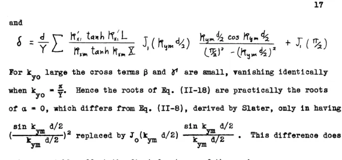
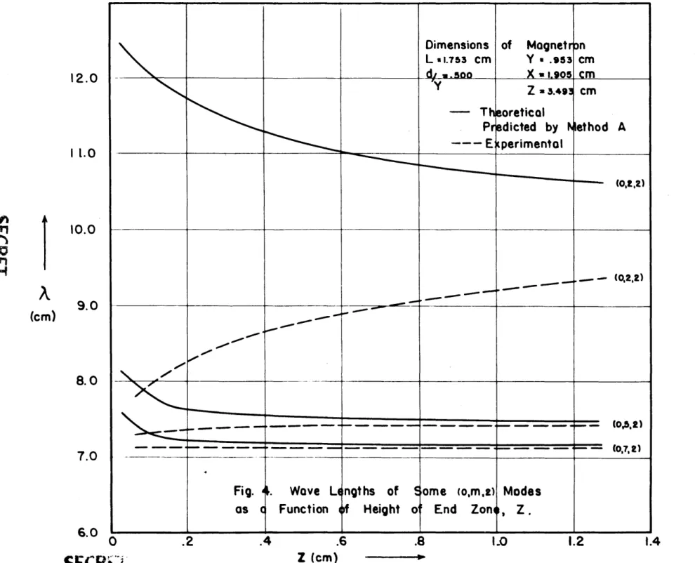
The calculated resonant wave length, X = 2x/ k ,2 + k z , for a 10 slot linear magnetron is plotted in Figs. 4 and 5 as function of the size of

12.0

11.0

.4

.6

.8

LO

1.2

1.4

Dimensions of

Magnetron

di ..

oo

X 1.0

iosCm

T oretical

P dicted by

Slethod

A

-E lperimental

Fig.

Wove Lengths of

Eome

(o,m,t) Modes

as

c

Function

of

Height o" End Zont, Z

.

(A

mn

I

10.0

9.0

(

(cm)

8.0

7.0

6.0

0

.2

10.0

9.0

L = 1.753

Cm

Y

a

.953 cm

d/.

cm

---

Theoretical

-edicted .

ethod

A

E perimental

Fig.

Wave

Lengths

of

Some

Modes

as

Function of

Height

of

End

lone,

Z.

I

x

8.0

(c m)

7.0

6.0

5.0

4.0

mi

- E

SECRET

21 the end zone, Z, for several values of m. Also shown are the results

of experiments on such a linear magnetron, to be discussed in the next

sec-tion. The predicted values do not agree qualitatively with experiment, since the measured wave length decreases as Z-9'0 whereas Eq. (11-22)

predicts increasing wave length. For large Z there is surprisingly good quantitative agreement for the (0,5,2) and the (0,7,2) modes. This agreement must be considered accidental, for it is at such values of kz that tan kzz is almost infinite. In general the method outlined does not yield a satisfactory solution of the problem.

Method B The second method tried is essentially a variant of

method A and will not be discussed in detail. It considers the problem

as one of a wave guide with a periodic array of T-Joints. The fields in the oscillator cavities are the same as those previously used except that the antisymmetrical component is neglected. In the end zone 'partial' fields, corresponding to each slot, are set up such that the tangential

electric field of each partial field matches the field in the slot and

vanishes everywhere else in the z = z plane. At large distances from its slot each partial tangential magnetic field has the form of a traveling wave corresponding to a (T.E.)1,0 mode propagated in the end

zone. In addition there are higher modes generated at the edges of the

slot which decay rapidly away from the slot. The total magnetic field

is the sum of these partial fields and the average of this total field

SECRET

22

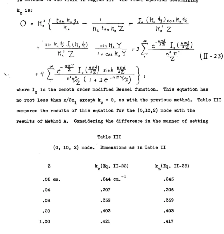
is matched to the field in Region II. The final equation determining kc is: z

0

tah

N

₂

f

_Z

1

Z

a7

where I is the zeroth order modified Bessel function. This equation has no root less than x/2z1 except kz = 0, as with the previous method. Table III compares the results of this equation for the (0,10,2) mode with the

results of Method A. Considering the difference in the manner of setting

Table III

(0, 10, 2) mode. Dimensions as in Table II

kz (Eq. 11-22) .244 cm. .307 .359 .403 .421

up the fields, the close agreement is surprising. This nothing new. kz (Eq. 11-23) .245 .306 .359 .403 .417

method thus yields Z .02 cm. .04 .08 .20 1.00

-U

SECRET

23 Method C In the previous methods the fields in the end zone

are connected with those in I only indirectly, through the oscillator

cavities. Yet the end zones and Region I really form a continuous region.

Region III can be considered as a part of I that has been bent at 90.

The error of the previous methods must lie in the omission of a factor insuring the continuity of these regions.

The simplest way of directly connecting Regions I and II is to require the continuity of the tangential magnetic field, B , at the junction of the two regions, namely, at the edge of the vanes defined by

Z = z and x - X. This condition has some simple pbysical interpretations. It states that the electric potential of the edge is the same whether

approached from Region III or Region I. Equivalently, it requires that the currents along the face of the vanes in the z-direction join on smoothly to the currents in the x-direction along the top of the vanes. It is easy to see that this condition results in a qualitatively correct answer. If the tangential electric field E is properly matched between

y

II and III, it can be shown simply from Maxwell's equations that the ve1rtical component of B is also matched. It then follows from div B = 0 that the flux of Bz at the boundary between II and III is equal to the flux of B in III, minus the small amount of flux of B 'leaking' from

y x

III into IV. Since the ratio of B to B is very small when k is small,

k 2 y

approximately k z , this leakage flux is negligible. Hence the flux

yo x

of B in the oscillator cavities is 'converted' almost entirely into_z flux of B in III. As Z decreases, the same amount of flux is crowded

y

SECRET

24 varies as sin k zz, that requires kz to increase as Z becomes smaller.

This is in rough agreement with experiment.

The calculation of kz according to this procedure will be carried out omitting edge effects, i. e., the fields in the oscillator cavities will be assumed constant across the width of the slot. The field components that are needed are;

in Region I:

a

e

in the

jth

BU

=k?

b~e

cak

x-

L)cs

and in Region III:

Z. Ccosh -gal< cas (-l

The expansion coefficients am and cm are determined as before by matching

+1v~ i .JT M;K .

the tangential component of the electric field, E , to the field in the oscillator cavities. The details of this calculation are similar to those in the previous matching between I and II and only the results need

be given:: With these

a,

Y

SECRET

s in T)'

L

C

o= -

-b

cos

z,

Y

,

}R

(f-2

7)

the edge z = z1, x = X becomes:

9

too

,m Y

s;I)X'L

eSi

(

IT-/

2 )

K , /2l

Since the matching cannot be done exactly, we match the average of B

y across the width of a vane. From Eq. (11-28) this average in Region I is

I

N

(,,X)

J

YCo

itm

-

_{C ,}

.

sinox-

si"

_(m

_{- 29)}

where D = Y - d, the width of a vane. Similarly, in Region III B at

the edge is

t0

b

0

X

,

Cos

xL

and the corresponding average is

-

_B

->9

-

.

-

e

e

-0_,

Y

tanh N,,X

sin

e

try

Ny D/2

The transcendental equation for k is found by equating these two averages: zM K ' h'mtank

h,,a

;.

t

_Z

I4V,

11/2

lw z

fl

f

-SECRET

(1[-30)

K

5j

(

,,X):..

F

_SECRET

26 If Z and the mode index m are large, so that k -~ k"zo~ km

and the hyperbolic tangents are practically 1, then the two series are

almost identical and Eq. (11-30) reduces to

S taii , = X

(1-Z

_tan

_T,'L

.

Another simple expression can be obtained if k is small, since then

k is approximately -k and kM is almost equal to k *-m In each

series the mth term therefore cancels the -mth term, leaving only the zeroth term. 'When k _yo is small

!g

0'/2D

~ ~

~

1

a

and the relation between k and k ', Eq. (11-8), can then be written as:

j o

x)

Y fi|

tan

L

With these simplifications Eq. (11-30) becomes

W~,erc

_trZ/r

₂

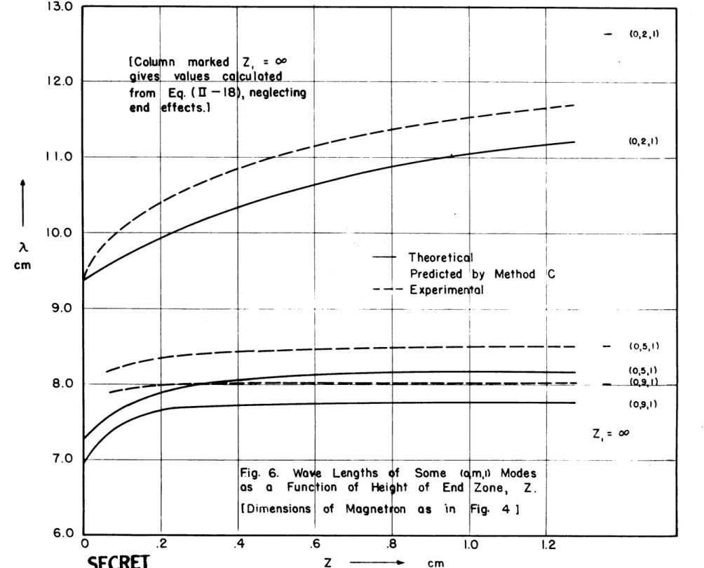
The calculated wave lengths of some (Om,1) modes in a 10 slot linear magnetron are plotted in Fig. 6 as a function of end zone height Z. They

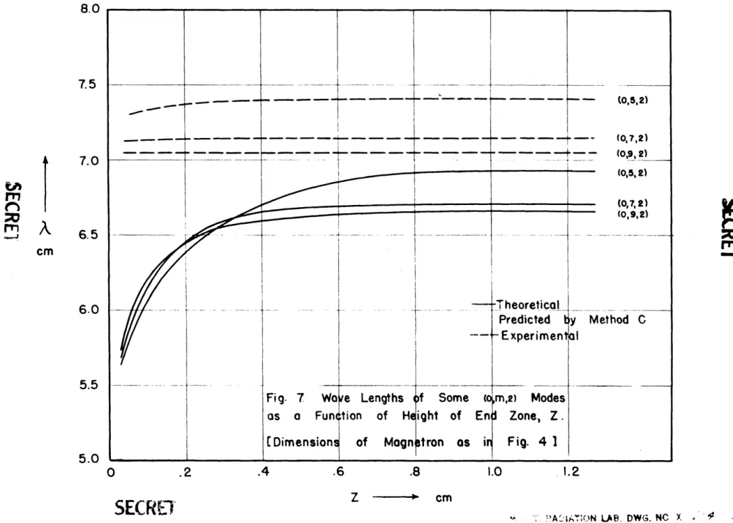
are computed from Eqs. (11-18) and 11-30). Also plotted are the experi-mentally measured wave lengths. Fig. 7 is a similar plot for (0,m,2) modes. The agreement is qualitatively correct since the calculated wave lengths decrease with decreasing Z, but the calculated values are always too small.

When the mode index m is small, the wave lengths disagree by about 4%. Since the measured end effect is only 8% at large Z for these modes, the relative error is quite large.

13.0

[Colunn

marked Z,

= 00

12.0

gives

values caculated

from Eq. (

- 18), neglecting

end effects.1

11.00

cm

---

Theore

Predic,

-W- E

xperi

9.0

8.0

7.0

Fig. 6. Wave Lengths

f

Some

as a

Function of Hei ht of E

[Dimensions

of Magnet on as

6.0

7.5

-_

I

-

zz~---

to,,2

7.0

6.5

-0

cm

6.0

---

--

--

Theoretical

Predicted

by

Method C

---

Experimental

5.5

-_-_

Fig. 7

Wo e Lengths

of

Some

to,m,2)

Modes

as

a Funetion

of

Height of End Zone, Z.

[

Dimensions

of

Magn tron as i

Fig. 4 1

5.0

-m

SECRET

27 Due to the uncertainty in the 'fringing' corrections the

magnitude of the end effect for higher modes is ambiguous. The measured wave lengths even appear to be a trifle higher than those calculated neglecting end effects. At most the end effect for these modes is about

1%. However Eq. (11-30) predicts an effect of more than 3%,

This large discrepancy is not surprising since the calculation completely neglects the higher modes generated near the edges. If we attempt to introduce these higher modes through the field given in

sin k d/2

Eq. (11-9), the chief change is to replace k 2 by T 0(k d/2), ym

which has a negligible effect. But it is evident that this in not a consistent method of taking the higher modes into account. This field corrects only for the effect of the edges at z = zl, and at x = X. However

the higher modes generated near the edge of the vane at the junction of Regions I and III must have a much larger effect. It is believed that these higher modes arise in the following manner. Eq. (11-6) gives k x as a function of k Y . Heretofore only the lowest root of this equation has been used. Due to the periodicity of tan k 'L higher solutions do exist. They have a variation in the z-direction given by

and k is therefore imaginary. These solutions thus are important only z

near z - z and decay rapidly away from these planes.

However there seems to be no simple way of including these

higher modes in the calculations, since we have no way of assigning ampli-tudes to each solution. The problem is complicated as these solutions are not orthogonal in any range. The only feasible method would seem to be a rather laborious variational procedure.

SECRET

28 III. Experimental Study of a Linear Magnetron

1. Description of Apparatus

In order to investigate experimentally the effects of the end

zones a 10 slot linear magnetron has been constructed, and its resonant modes measured.

Details of the construction are shown in Figs. 8, 9, and 10, and the important dimensions are sunmarized in Table IV.

Table IV

Dimensions of Linear Magnetron

L - 1.753 i .005 cm. d .476 ± .003 cm. Y .952 ± .002 cm. X - 1.905 + .010 cm. 2z, - 3.493 ± .003 cm. Z - 0.0 to 1.27 cm.

The slots are milled in a brass plate 1" thick fastened to a similar brass plate. This solid base reduces distortions due to strains produced in milling. At each side of the plate the vanes are cut away to form ledges

1/2 " wide. Bolted on to the ends of the plate are 1/2 " brass end-plates,

each containing five holes permitting the insertion of loops at various positions. The slots at the ends of the plate are cut half width, so that

EECRET

lan

-0

O0

O0

O

0

0--End

Plate

0O0

O

I

0A

O0

____I

I P..I

O0

O0

0

Elevation

Smd Plate

I

F

0-01

0

0

0

0

-0

0

=.o

33

-)

Plan

,Tapped

v for

Holes

Loops

-O0

Elevation

a

0

0

Fig. 8

b

I

-SECRET

9

St

&

N

g0

r

4%

N

tN ., S

f/9

0 6' Val I-4 Sm ~ -r

SECREI

29

together with their images in the end plates they constitute slots of

normal width. Fitting in notches cut at the top of each end plate are two bars stretching from one plate to the other. These cross bars help to anchor the brass plates which form the sides of the cavity. The side plates carry blocks of varying thickness, as shown in detail in Fig. 8b, which fit rather tightly between the ledge and the cross bar. The spaces

between the vanes and the blocks constitute the end zones. The size of the end zone can be changed by varying x, the thickness of the blocks. The positions of these blocks and of the end zones are clearly shown in Fig. 9. It was thus possible to vary Z in eight steps from .013 cm. to

1.27 cm. A slotted cover plate completes the cavity. Two plates were

used, one with a slot in the middle, the other with the slot displaced

1" from the center. The standing wave pattern of the fields in

cavity was measured by a probe inserted in the slot. The completely assembled linear magnetron (including the probe holder, or carriage, and tunable probe) is shown in Fig. 10.

The experimental arrangement for the measurement of the resonant wave lengths is shown schematically in Fig. 11. In the region from 6.5 cm.

to 9.7 cm, a Western Electric 1332 CT (Samuel tube) was used, while the region from 8.7 to 13.0 cm. was covered by a Western Electric 707 A (McNally tube). Various types of probes were tried. The standard non-tunable wave guide probe designed for use at 10 cm. was used, with the

bolometer element replaced by a crystal. More sensitive was the tunable

10 cm. probe, kindly lent by Dr. Krutter, shown in Fig. 10. Many of the

SEfitT

Crystol

Lossy

Cable

Vve

Meter

or

Monitor

Fig. II

SECRET

Shunt

and

Galvanometer

Oscillator

cm

Linear

Magnetron

Lossy

Cable

- -+ to

SECRET

30

tuner constructed of standard Sperry fittings, which proved most sensitive of all. Wave lengths were measured with a Radiation Laboratory Type 401 open end coaxial wavemeter, which is stated to have an absolute accuracy of .1%. Readings could be reproduced to a much smaller error, about

.02 to .03%. The galvanometer used to measure the currents in both the output loop and the probe was a Rubicon galvanometer,

sensitivity = 3.0 x 10~9 amp./mm. The greater sensitivity compared to the

more customary microammeter was essential for the investigation of the higher modes, since the fields at the probe are very weak.

Several minor changes were often made in the set up shown in

Fig. 11. Thus whenever possible the wavemeter and monitor were

simul-taneously connected to the r.f. line through a reaction coupler, essen-tially a T-joint. This arrangement, while very convenient, could not be used often as the sensitivity was then greatly reduced.

2. Discussion of Method and Results

The technique of cold resonance measurements has been described

by Slater , Tonks and Crawford and others, and need be given only

briefly. Resonances are detected by means of an output loop, similar to the input loop. The index m of the mode is given by the number of maxima

in the standing wave pattern measured by the probe. The (0,m,1) modes are distinguished from the (0,m,2) modes by the difference in the method of excitation. If the input loop is in the center, i. e., in the z - 0 plane (Fig. 3), only the (0,m,l) modes are excited, while if the loop is

---T. C. Slater, Radiation Laboratory Report 43-9

(8)L. Tonks and S. N. Crawford, General Electric Research Laboratories, report dated 7/15/42

- m

SECRET

31 placed off center both the (0,m,1) and (0,m,2) modes are generated.

Similarly, when measuring a (0,m,2) mode the slot for the probe, and the output loop must be placed off-center, as shown in Fig. 10. In practice two output loops were used, one in the middle and the other in the

outer-most hole. If the resonance could not be detected in the center loop,

it definitely belonged to a (0,m,2) mode. By these means it was often possible to distinguish a (0,m,2) mode from a nearby (0,m,1) mode even though the two were much closer than the width of the resonance curve.

Energy could be radiated from the slot in the top plate when

in the off-center position. This was prevented by a brass plate cut to fit around the probe carriage and so arranged as to cover all of the slot not covered by the probe and its holder.

Beside the slot for the probe the cavity differed from the ideal geometry of Fig. 3 by the presence of the cross bars and loops. The cross bars are in Region IV where the fields are very weak and hence,

as Slater 9 has shown, should affect the resonant frequencies only slightly. In one experiment the cross bars were temporarily removed without changing the wave length of the (0,3,1) mode by more than .05%. The loops, each less than .02 cm.a in area, likewise had neglibible

effect. Several times the input and output loops were withdrawn until they were practically flush with the wall. The currents decreased by

a factor of more than one hundred, but the resonant wave lengths remained

unchanged to within .002 cm. The width of the resonance curve was also unaffected. Because the cavity and wavemeter were simultaneously connected

to the oscillator little trouble was experienced from 'pulling'.

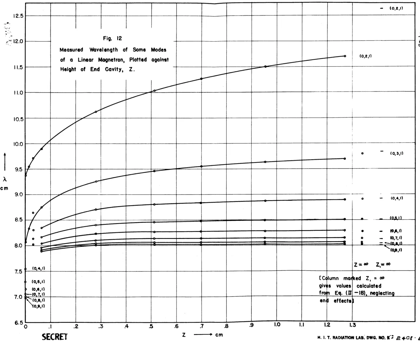
32 The results are presented graphically in Figs. 12 and 13, and the actual measurements are tabulated in Appendix II. In Fig. 12 the column of dashes marked z = co are calculated values assuming the oscillator

cavities so long that end effects may be neglected, i. e., kz = 0. The edge effects as corrected by Eq. (11-18) are included in these values.

The points marked Z = oo were experimentally measured by removing the side plates. They differ only slightly from the wave lengths for Z = 1.27 cm.

The (0,1,1) mode was never found as it must be above the range of the oscil-lator. The (0,10,1) mode could not be detected and the (0,10,2) mode

was found only for Z = 1.27 cm. and Z = co . These modes were apparently so weakly excited that they were often lost in the resonance curve of the neighboring m = 9 mode. In the two cases in which the (0,10,2) mode was

found, its amplitude was 1/8th of the (0,9,2) mode. Modes whose index n

is greater than 2 have wave lengths in general that are outside the range of the oscillator. However, a mode occurring at about 6.9 cm. is believed to be the (0,2,3) mode.

As the result of an error in machining the blocks attached to

the side plates did not make contact with the ledge, i. e., with the

x - x + L plane. The gap between the two was sometimes as much as .004". To correct the situation the blocks were silverplated to a thickness of

.006". They were then too large for the space between the crossbar and

the ledge. To insert them the crossbar was loosened slightly, until the block could slip in, and then screwed down tightly. It was hoped in that way to insure contact between the metal surfaces. A conducting grease, "Lubriplate" was also used between the surfaces. The magnetron could be taken apart and reassembled without any noticeable change in the resonant

Fig. 12

12.5

12.0

11.5

11.0

10.5

10.0

9.5

.1

.2

.3

.4

Modes

against

.5

.6

.7c

z

cm

.8

1.0

[Co

giv

fra

en i

1.1

lumn

mat

Is

values

Eq. (H

effectsl

1.2

ked

Z, =

00

calculated

-18),

neglectin

Measured

Wavelength of Some

of a Linear Magnetron, Plotted

Height of End Cavity, Z.

x

cm

9.0

8.5

-

8.0-7.5

-7.0'

6.5-0

9.5

-

9.08.5

-8.0

7.5

-70

-

6.5-

6.0-0

11.5

11.0

10.5

10.0

Measured Wavelength of Some

of a Linear Magnetron, Plotted

Height of End Cavity, Z.

.2

.3

.4

.5

Modes

against

.6

.7

.8

.9

L.O

1.1

Fig. 13

LUJ

cm

.1

1.2

SECRET

~33

frequencies. However the condition of the Lubriplate film showed that

the blocks for Z = .030 cm. still did not make contact. It will be noticed that the points for this end zone in Fig. 12 are definitely too high. For Z about .3 cm. and larger the effect of the gap is small, the correct wave length being at worst .6% lower for the (0,1,2) mode than when the gap is present. As Z decreases the error increases to several per cent for (0,m,2) modes at Z = .08 cm. In fact, elimination of the gap changed

the qualitative behaviour of the (0,m,2) modes. When the original blocks were used, it appeared that the wave lengths increased as Z became very

small. After the blocks were silverplated, it was found that the wave lengths actually decreased slightly, as shown in Fig. 13.

At very small values of Z the measurements became quite diffi-cult. The patterns measured by the probe became unsymmetrical and distorted, and slight differences between the sizes of the end zone on each side

destroyed the distinguishing symmetries of the (0,m,1) and (0,m,2) modes. The intensity of the modes also decreased quite rapidly. At Z - .030 cm.

few modes were recognizable, while at Z = .013 cm., only the (0,2,1) and (0,3,1) modes could be detected at all. It is unfortunate that

measurements could not be made in this region. As far as the measurements went the wave lengths of the higher modes did not seem to change appreciably with Z. However if the wave lengths are to reach their proper limiting values at Z = 0, they must drop sharply at least 1 cm. for a further

change of Z of .06 cm. It is possible, therefore, that the modes cross over somewhere in this region.

The limiting values for Z = 0 were measured as follows. With

r

SECRET

34 fastening the side plates to the magnetron were loosened so that a copper foil .010" thick could be inserted in the gap. The screws were then tightened as much as possible. It is certain that the tops of the vanes were in contact with the copper foil. "Lubriplate" was also applied to all surfaces. In Table V the results for the (0,m,1) modes

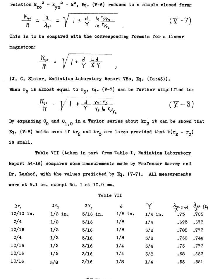
are given. Also tabulated are the calculated wave lengths found from

12 Tr

The values in the third column are calculated from k * as given by

Eq. (11-8), while those in the fourth column are corrected for edge

effects as given by Eq. (111-18).

Table V

Resonant Wave Lengths for Z = 0

Mode 0,2,1 0,3,1 0,4,1 0,5,1 0,6,1 0,7,1 0,8,1 0,9,1 Exp. 9.378 8.071 7.548 7.298 7.156 7.063 7.004 6.977 Theor.(Eq. 11-8) Theor.(Fq. 11-18) cm. 9.42 cm. 8.09 7.57 7.31 7.16 7.07 7.019 6.992 9.37 8.04 7.51 7. 26 7.12 7.03 6.97 6.95 cm.