Publisher’s version / Version de l'éditeur:
Building and Environment, 27, January 1, pp. 39-49, 1992-01-01
READ THESE TERMS AND CONDITIONS CAREFULLY BEFORE USING THIS WEBSITE. https://nrc-publications.canada.ca/eng/copyright
Vous avez des questions? Nous pouvons vous aider. Pour communiquer directement avec un auteur, consultez la première page de la revue dans laquelle son article a été publié afin de trouver ses coordonnées. Si vous n’arrivez pas à les repérer, communiquez avec nous à [email protected].
Questions? Contact the NRC Publications Archive team at
[email protected]. If you wish to email the authors directly, please see the first page of the publication for their contact information.
NRC Publications Archive
Archives des publications du CNRC
This publication could be one of several versions: author’s original, accepted manuscript or the publisher’s version. / La version de cette publication peut être l’une des suivantes : la version prépublication de l’auteur, la version acceptée du manuscrit ou la version de l’éditeur.
For the publisher’s version, please access the DOI link below./ Pour consulter la version de l’éditeur, utilisez le lien DOI ci-dessous.
https://doi.org/10.1016/0360-1323(92)90006-B
Access and use of this website and the material on it are subject to the Terms and Conditions set forth at
Influence of computational parameters on the evaluation of wind
effects on the building envelope
Baskaran, B. A.; Stathopoulos, T.
https://publications-cnrc.canada.ca/fra/droits
L’accès à ce site Web et l’utilisation de son contenu sont assujettis aux conditions présentées dans le site LISEZ CES CONDITIONS ATTENTIVEMENT AVANT D’UTILISER CE SITE WEB.
NRC Publications Record / Notice d'Archives des publications de CNRC:
https://nrc-publications.canada.ca/eng/view/object/?id=a30aee44-14c5-4c38-b68b-e38eaff9f6cd https://publications-cnrc.canada.ca/fra/voir/objet/?id=a30aee44-14c5-4c38-b68b-e38eaff9f6cdR e f
-1
.
5
U
P
r
Z
PUB
2
-- - - ..- -National Research
Conseil national
Council Canada
de recherches Canada
Institute for
lnstitut de
Research in
recherche en
Construction
construction
Influence of Computational
Parameters on the Evaluation of
Wind Effects on the Building
-
Envelope
by Appupillai Baskaran and Ted Stathopoulos
ANALYZED
Appeared in
Building and Environment
Volume 27, Number 1
p. 39-49, 1992
(IRC Paper No. 1753)
Reprinted with permission from
Pergamon Press
NRCC 33969
MAR
-
1\92
B I B L e ,
. s ~ Q U E
I
I A E
m1RC-
ImTBuilding andEnvironrnent, Vol. 27, No. 1, pp. 3949, 1992
Printed in Great Britain.
036&1323/92 $5.00+0.00 Pergamon Press plc.
Influence of Computational Parameters on
the Evaluation ofwind Effects on the
Building Envelope*
APPUPILLAI BASKARANt T E D STATHOPOULOSS
This paper sys!emoricrrlly c.mmines the iqffuellr:e qf !he comprirational parnmPfer,c on !he cotnpured wind londs nn the htrildi~~g P I I I ! P / ~ ~ Y . Paramrfers considered ificlurle: size
nf the compularinnal
domain. nundwr #f cromyuiotionnl grid nodes, criteria rcr~il for i h ~ ror~l*e~yerrcc q f n n iterating pmcess und computing rintt, r~qtri~.enren/s ,for diflercnr conlpzi!er rystems. In all fotrr eases, cornpried rea1i11.v and campuratic~~tul co.rt (C PI! lintr I arc nnu/~*=ednnc?fi)r some caws compuri.rons are oI,~o mu& wifh the ~ x p r r i m m t n l durn. 3.v using 1hi.r nna/ysi.~ o r/ir~gno.rtic system to nlonilor the computed results can be developed.
L np NX, NY, NZ
NOMENCLATURE
hybrid difference scheme coefficient at node P
building width
mean pressure coefficient building height
turbulence kinetic energy
recirculation length from leeward side of build- ing
building length
number of nodes surrounding P
total nodes on x , y and z directions fluid pressure
grid node under consideration imbalance in the conservation of mass residual source
linearized source term time
mean velocity components along x, y, z direction velocity at gradient height
velocity at roof height
distance along the co-ordinate axis height of the boundary layer
Greek symbols
ax, dy, 6z grid distances between nodes
E dissipation of turbulent kinetic energy
I I$ dependent variable, i.e. u, o, w, k, E
Abbreviations
USD Up-Stream Distance
.'
DSD Down-Stream DistanceDT Distance from the building Top
-.
DS Distance from the building SideMIPS Millions of Instructions per Second.
1. INTRODUCTION
A SYSTEMATIC approach is necessary t o understand the products of nature and their consequences in human life. Wind is not only a n integral part of human survival, it also has significant effects when it flows around build- ings. Three major wind-induced effects o n buildings (structural, environmental and energy) are listed in Fig. 1. It is the responsibility of a building engineer to design a safe and economical building taking these effects into consideration. So engineers need information regarding these wind-induced effects o n buildings during the design process. This information is available through wind load- ing standards and codes of practice, which are based o n data from various systematic wind tunnel experiments, sometimes confirmed by full scale measurements.
Improvements in computer resources offer a new and feasible tool for the evaluation and understanding of wind effects o n buildings. However, it was only recently that studies (Vasilic-Melling [I], Hanson et al. [2, 31, Summers et al. [4], Paterson and Apelt [5, 61, Murakami
et al. [7, 81, Mathews and Meyer [9], Baetke [lo], Baskaran and Stathopoulos [l I] and Baskaran [12]) have been made to simulate wind flow conditions around buildings using computers. This lack of utilization of the booming computer resources by the wind engineering research society is probably due to not only the com- plexity of the problem but also the difficulties involved in numerical modelling of the turbulence process, as explained by Hunt [13].
.-
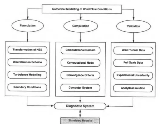
Numericallv simulated results depend o n many factors. *The authors prepared the paper on behalf of the National A diagnostic system is often necessary t o monitor the
4- Research Council of Canada, and therefore the copyright in the
computed results. Numerical modelling of wind flow Con- paper belongs to the Crown in right of Canada, i.e. to the ditions around buildings mainly consists of three stages
Government of Canada. of operation, as shown in Fig. 2. These are : formulation
'y Institute for Research in Construction, National Research
Council of Canada, Ottawa, Ont., Canada, K1A OR6. stage, computation stage and validation stage. Each stage
1 Centre for Building studies, concordia university, involves various sub-stages, some of which are displayed
Montreal, P.Q, Canada, H3G 1M8. in the figure. The diagnostic system should be capable of
A . Baskaran and T. Stathopoulos
Fig. 1. Perspective of wind induced effects on buildings.
identifying and filtering the error introduced during each of these processes.
For the formulation stage, research efforts [14] have been made in the past to identify the influence of the various approximations of the Navier-Stokes equations. Raithby [15] critically evaluated different schemes used for the convective term interpolation and three schemes
were also applied and compared for the computation of steady state recirculating flows by Leschziner [16]. Turbulence modelling has also been well scrutinized by the computational group of Imperial College of Science and Technology in London [17, 18, 191. For engineering applications, the well known k-E models are found to be the ideal choice, considering the computational cost and the accuracy of the computed results. Authors who con- tributed to Building and Environment (Vol. 24, No. 1, 1989) Special Issue, "Numerical Solutions of Fluid Prob- lems Related to Buildings, Structures and the Environ- ment" were also in favour of k--E turbulence model for the wind flow conditions around buildings.
Validation of the computed results is also an integral part of the numerical simulation. It can be performed by comparing the results with full scale measurements or, more often, by using data from wind tunnels. Summers and co-workers [4] performed a direct validation process for their simulated results. For comparison purposes, a simple wind tunnel model was fabricated and pressures and velocity were measured at the same locations as the computation [20]. Extensive comparisons in Ref. [4] clearly show the complexity involved in the validation stage, even for a simple building configuration. To exclude the modelling problems in the wind tunnel such as scale effects and turbulence intensity, Richards [21] compared the computed results using the data from a full
.
scale "experimental station" on a low-rise building. His computed results were obtained by using Spalding's com- mercial code PHOENICS [22].In this paper a systematic analysis has been made to identify the influence of computational parameters on the computed wind effects on buildings. Considered par-
I
Numerical Modelling of Wind Flow ConditionsI
1
Transformation of NSE-
Discretization Scheme-1
Turbulence Modelling-1
Boundary Conditions1
1
Computational Domain1
(
Computational Node)
( Convergence Criteria )(
computer system1
Wind Tunnel Data
Full Scale Data
( Experimental Uncertainly ) Analytical solution
+
Dlagnostlc System
A
Fig. 2. Components of a diagnostic system for the numerical modelling of wind flow conditions around buildings.
Computational Parameters and Wind Efects on Buildings
ameters include the size of the computational domain, the number of computational grid nodes, the criteria used for the convergence of an iterating process and computing time requirements for different computer sys- tems. In all four cases, both the computed results and the computational cost (CPU time) are analyzed; for some cases, comparisons are also made with the experimental data. Due to the complexity of the problem considered, observations are summarized based on the analysis of these parameters and no general guidelines are formu- lated. However, using these observations, one can develop a diagnostic system to monitor the computed results. The following section present a brief summary of the computational methodology, whereas the rest of the paper is dedicated to the analysis of the computational parameters.
2. COMPUTATIONAL METHODOLOGY
This section only outlines the computational pro- cedure; more details can be found in Baskaran [12]. By using the control volume method of Patankar and Spalding [23], the differential equations are transformed into difference form. The final algebraic equation is written :
in which P is the grid node where the dependent variable
4,
is computed, n, is the number of nodes surroundingP, a, is the hybrid difference scheme coefficient and S, is the linearized source term.
The well known SIMPLE algorithm of Patankar [24] is used to correct the velocity field and also to improve the initially assumed pressure field. The advantageous staggered grid arrangement is used. For boundary con- ditions, the wall functions of Launder and Spalding [25] are used for the velocity variables and the newly developed zonal treatment method of Stathopoulos and Baskaran [26] is used for the turbulence variable to bridge the boundary nodes with the computational domain.
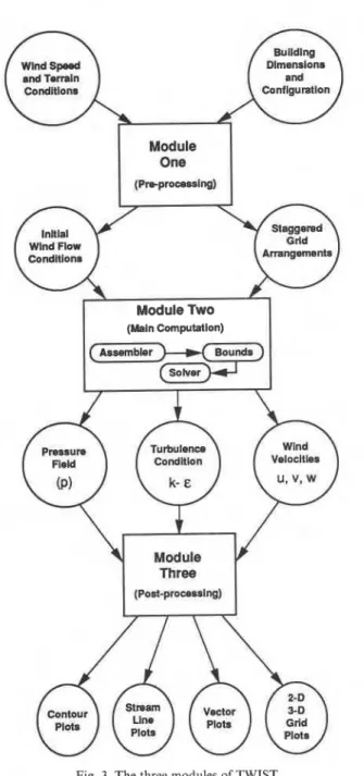
All computations were performed using the computer code TWIST-Turbulent WInd Simulation Technique- which consists of three modules respectively performing pre-processing, main computation and post-processing shown diagrammatically in Fig. 3. These three modules coded in ANSI Fortran-77 can run individually or in sequence. The post-processing module 3 frequently calls appropriate graphics subroutines during its operations. Modules 2 and 3 need more computer storage capacity in comparison with module 1, whereas module 2 takes the highest CPU time among the three. The main advan- tage of the modular structure is that the user can extend the code for any particular problem of interest, by adding new modules to an existing one.
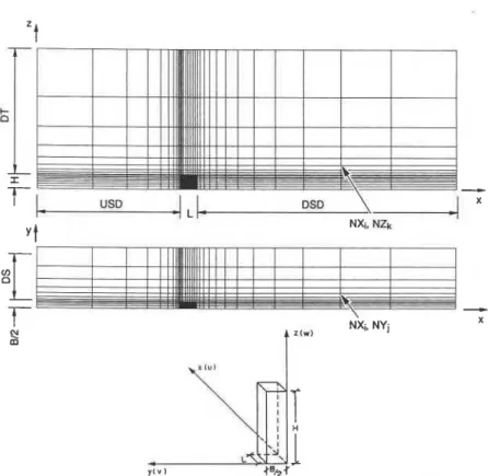
A single building model about 14 cm high and 15 x 15 cm cross-section (56 x 60 x 60 m in full scale) is con- sidered as the test case. Computations are performed for a power law inlet velocity profile having exponent 0.16, with a free stream wind speed of 12 m/s at a wind tunnel gradient height of 60 cm. Figure 4 shows a typical grid cluster for the considered test case, both in plan (xy) and
Module One (w-lnp)
1
Module TWO1
(Main Computation) bsrmbler ModuleY - d
Fig. 3. The three modules of TWIST.
sectional (xz) views ; the grid distances Sx, Sy and Sz are not equal. Indeed, a non-uniform grid is often desirable. The misconception that non-uniform grids lead to less accuracy than uniform grids has no basis. In general, an accurate solution can be obtained only when the grid distribution is sufficiently fine. There is no need to use a fine grid in regions where the dependent variable changes rather slowly, such as the velocity above the gradient height. On the other hand, a fine grid is required near the windward wall or the roof of a building for numerical approximation of the high gradients. These basic ideas are taken fully into consideration during the grid gen- eration, as can be clearly identified from the figure. More- over, by using less grid spacing near the solid boundaries and arranging for non-uniform spacing in other regions, the efficiency of the computation is increased.
A. Baskaran and T. Stathopoulos
't
USD L DSD\ A x
y t NXiPFig. 4. Computational mesh distribution and co-ordinate system used.
The co-ordinate system used in the computational pro- cedure is also indicated in Fig. 4. The x-axis carries the streamwise velocity; the lateral and vertical velocities follow they and z directions, respectively. An Up-Stream Distance (USD) from the windward wall and a Down- Stream Distance (DSD) from the leeward wall define the boundaries of the computational domain along the x direction. For other directions, distances DS and DT are used as shown in the figure. Note that (NX,, NY,) is a node in the plan view (xy direction) which has (NX*NY) total nodes. Similar explanations also apply for sectional view.
3. EFFECT OF COMPUTING PARAMETERS The effect of computing parameters is addressed by considering four main factors of the computation stage (see Fig. 2) : size of the computational domain, number of computational nodes, criteria of terminating the iteration process and the use of different computer systems. 3.1. Znjuence of domain size on the computed results
The influence of the domain size is analyzed first, because experimental data are available which can be used as preliminary information for the numerical solu- tion. Systematic studies (Hunt and Smith [27], Hunt [28]) were initiated during the early 70s for the understanding of wind generated wakes around a building and were continued by Lemberg [29], Penwarden and Wise [30] and Gandemer [3 11. Beranek [32] grouped some of these results for the determination of the influence area for wind flow around tall slender buildings, tall buildings of transitional type, which have a significantly smaller
dimension along the flow direction than along the other two directions, and long buildings. These general guide- lines are taken into account by the present study for the determination of the computational boundaries.
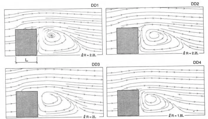
As listed in Table 1 four domain sets are considered in the analysis. The extent of the computational domain along the x, y and z directions is shown for each domain. During this exercise, other parameters namely the total number of nodes (81,600) and the convergence criterion (0.2) are kept constant. The DD2 set is selected based on the 2-D experimental study by Antoniou and Bergeles [33] and Bergeles and Athanassiadis [34] and it is con- sistent with the previous computational work of Paterson [5, 61 and Murakami et al. [7, 81. With DD2 as the base, the effects on the computed results of increasing as well as decreasing the domain size were analyzed.
Figure 5 shows the streamline plots for the four cases considered. These plots show the side view pattern of flow distribution for a plane passing along the center of the building which is exposed to normal wind flow conditions. The plots are obtained using the converged
Table 1. Specifications of the different computational domains
.-
used in the present study
.
X Y z
Set USD DSD DS DT ,
Number of nodes : 8 1,600 Convergence criterion : 0.2
Computational Parameters and Wind Efects on Buildings 43
Fig. 5. Side view of streamline plots for different computational domains.
velocity components u and w. In all four figures the incoming flow separates from the leading edges and then forms recirculations behind the building. Overall, no significant differences are noted among the four figures. However, the recirculation zone of DD4 is smaller in comparison to the others. To quantify these changes, the length of recirculation is calculated as explained in Vasilic-Melling [I], by specifying the distance from the leeward wall, to the point where ulu, = 0.0. These locations can also be easily identified from the streamline
plots; the respective recirculation lengths were equal to 2.2 L, 2.2 L, 2 L and 1.8 L for DD1, DD2, DD3 and DD4. Increasing the domain from DD2 decreases the length of recirculation. To support this description of the wake flow behavior, experimental evidence of flows over buildings, such as flow visualization techniques, will be necessary.
The induced pressure values were also analyzed for the variation in the domain distances, as shown in Fig. 6 . The windward wall positive pressures, and suctions induced
WINDWARD WALL p 6 0 m + H=SSm 754
Lf5$
50. 1%) WIND1
DDi 25. A1
DD2 01 DDg x1
DD4 01
MEASURED ILEEWARD WALL SlOE WALL
44 A . Baskaran and T. Stathopoulos
Table 2. Specifications of the different grid distributions used in the present study
- -
Set NX NY N Z Total
Domain specification : DD2
Convergence criterion : 0.2
both on the leeward and side walls are shown in the figure. All the results are presented in the form of pressure coefficients, normalized by using the dynamic pressure at the building roof height. The maximum difference among the four sets was found for the pressure nodes near the ground level of the front wall. The DD1 curve is always away from the others, irrespective of the building wall and the pressure coefficient values are not significantly affected when the domain distances are increased beyond DD2. When comparing the observations of this figure, including the experimental results, selection of DD2 domain for further examination of the problem appears to be a good choice. In addition to the changes in the numerical solution, the economic aspects of the com- putation are analyzed and discussed below.
The CPU time requirements, which are obtained under batch mode operation of the VAX11.2 computer system, are analyzed; an increase in the domain distances increases the necessary CPU time requirements.
3.2. Influence of number of nodes on the numericalsolution
In the previous section, the effect of computational domain was studied by analyzing the computed velocities and pressures. It is clear that the numerical solutions are rather insensitive for domains beyond DD2. The CPU time requirement also favors the DD2 domain selection. Thus this section presents the influence of the number of grid nodes on the numerical solution, keeping the domain constant as DD2. Four additional sets of grid systems are generated as shown in Table 2, by increasing as well
as decreasing the grid set NN4 that was used in the previous section. Table 2 also provides the number of nodes for each direction. As the total number of nodes of the computation increases, the number of nodes in each direction also increases. The number of nodes along the longitudinal direction (x) increases more than the number along the other two directions.
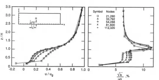
A typical location at a distance 0.05 L from the wind- ward wall of the building was selected to analyze the local effect of nodes on the velocity and turbulence ; the results are shown in Fig. 7. The vertical axis shows the node distance from the ground level normalized by the building height. Longitudinal velocity and square root of kinetic energy are normalized by the gradient velocity. Such non- dimensional values are shown in the horizontal axis. In both cases, the differences due to grids diminish with distance from the ground. Maximum turbulence values occur at z/H = 1.0, where the flow has high gradients due to its separation from the leading edge. The effect of the number of nodes on the velocities is clearly shown and this effect directly influences the computed turbulence values; these values are increased when the number of nodes are increased. On the other hand, for both vari- ables only minimum changes are observed when the grids increase beyond 81,600 (NN4). Similar observations have been made for the other locations of the flow domain.
Pressure values in coefficient form have also been com- puted for different grid systems. Among the three walls, the influence of the nodes is pronounced for the side wall, where the flow is complex. As noted for the velocities and turbulence, the set NN4 is numerically optimum if one considers all the walls. When comparing the results from various grid sets with experimental data, even the NN3 grid set may be considered sufficient for the compu- tations. However, further investigations and repetitive runs are necessary to generalize these observations.
Examination of the CPU time requirement in this case shows that the CPU time increases with an increase in the number of nodes. This may be due to additional operations needed by the process, to settle down. A simi- lar increase in the CPU time was also observed for each
2 0 0.2 0.4 0.6 0.8 1.0 0 5 10
u l ug
-
.Is;
,%ug
Fig. 7. Computed longitudinal velocity and turbulence intensity upstream of the building for different number of computational nodes.
Computational Parameters and Wind Eflects on Buildings
45
iteration and this can easily be explained by considering the increased number of arithmetical operations. More- over, the CPU time required is also influenced by the number of iterations performed, which itself increases with the number of nodes.
3.3. Effect of error level on the computed solution
For pressure-coupling schemes such as SIMPLE, the convergence of the numerical solution mainly depends on the under-relaxation factors and the acceptable error level of the solution. Patankar and Spalding [23], Gos- man and Pun [35] and Patankar [24] performed sen- sitivity analysis for the under-relaxation factors. A set of optimum values were recommended for separated flows with recirculations and these factors were used in the present computation. Therefore, the influence of the under-relaxation factors on the computed result is not examined. Before presenting an acceptable error level for the numerical solution, it is useful to explain the inter- relation of the term with the iterating procedure.
Conventionally, an iterating process is said to have converged when further iterations do not produce any change in the values of the dependent variables. Such a criterion may sometimes be misleading [3, 231. When a heavy under-relaxation factor is used, the change in the dependent variable between successive iterations is slowed down. This may create a false convergence image, even though the current working solution is far from convergence. One way to overcome this numerical illusion is by monitoring how well the discretized equa- tions are satisfied by the current value of the dependent variable and .this can be conveniently performed as follows :
The residue of a particular iteration for node P can be obtained from equation (1) as :
For a fully satisfied discretized equation, the L.H.S. of equation (2) has zero or near zero value. When
4,
takes the velocity variable (u, v and w) the calculated R, rep- resents an imbalance in conservation of momentum. Since for the present study, the continuity equation is solved by using the SIMPLE algorithm, R, will represent an imbalance in the conservation of mass. Similarly, with the turbulence variable (k or E ) , Rg represents an imbal-ance in turbulence quantities.
In the present study, the convergence criterion was obtained based on the normalized error. Using equation (2), R, for each node is calculated and at the end of each iteration the summation of R, for all nodes is obtained. This is the total error of the iteration for the respective variable. The total error obtained for the first iteration is called the initial error of the computation. Then the normalized error is obtained by dividing the total error of each iteration by the initial error. For example, a normalized error of 0.7 reveals that the iteration process reached a stage where the initial error is reduced by 30%. Such error levels are displayed in the vertical axis of Fig. 8, which has three curves representing the maximum value among the velocity variables (imbalance in the momentum), the error in pressure (imbalance in the con-
servation of mass) and the maximum value among the turbulence quantities. For the considered building geometry, the error is always higher in pressure than in the other variables. The same trend has been found for other buildings tested and this is probably due to the fact that a zero value is initially assumed for the unknown pressure field [24]. This is why most of the studies using the SIMPLE algorithm follow a convergence criterion based only on the imbalance of conservation of mass.
Another interesting feature observed in Fig. 8 is the reduction in error factor during the initial stage of the iteration process. A significant reduction of about 60% is found within the first 20 iterations ; this steep gradient in reduction tends to slow down for further iterations. An increase of about 30 iterations (from 50 to 80) only reduces the normalized error to about 0.05. Therefore, termination of the process after 50 iterations was found to be reasonable. However, its consequences on the numerical solution as well as on the computational cost must be discussed.
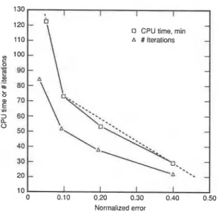
Computations were performed based on four con- vergence criteria (0.4, 0.2, 0.1 and 0.05) without speci- fying any upper limit on the number of iterations. The DD2 computational domain and the NN4 grid set were used. The convergence criteria have a more pronounced effect on the computational cost as shown in Fig. 9. As expected, both the iterations and the CPU time increase when the normalized error levels are reduced. Based on the available limited data points, the curve can be divided into two segments at a point 0.1 on the x axis. The curve is steeper for the x axis region up to 0.1 in comparison to the region beyond 0.1. Thus the computational cost will increase significantly if one requires an error level less than 0.1.
Furthermore, the computed pressure and velocity values were analyzed as previously and found insensitive for the error factor beyond 0.1. Differences were noted between the results of 0.4 and 0.1 while only marginal changes were found in the computed results for 0.2 and 0.1 sets. Thus selecting 0.1 as the normalized error factor is reasonable, considering both the computed results and the cost. However, further research efforts are necessary to validate this observation by changing the other parameters, such as building height and inlet velocity profiles.
3.4. Influence of various computer systems
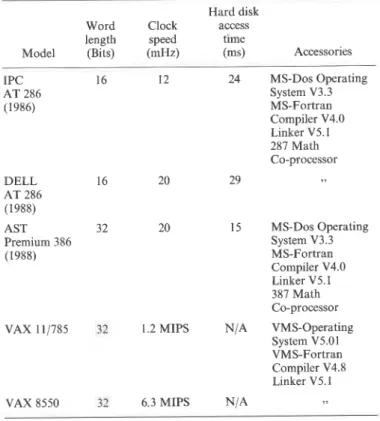
Computational runs have been carried out on three different micro-computers, namely AST Premium 386120, DELL 286120 and IPC 286112, as well as on two mainframes VAXl1.2 and VAXl6.3. The specifications of the computer systems used in the present study are given in Table 3.
Keeping the size of the computational domain constant, the number of control volumes inside the domain has been varied to establish the parameters for economical computation. Simulations were made on each computer system based on its capacity limits. Figure 10 presents the results; the CPU time needed only for module 2 is plotted as a function of the number of grid nodes (see Fig. 3). The CPU time for the microcomputers represents the direct, continuous access time whereas the CPU time for VAX machines is taken under batch mode
46 A. Baskaran and T. Stathopoulos 1 .O 0.9 0.4
Cn
0.7 k 0.6 Le
r=i 0 0.5::
-
-
0E
0.4 2: 0.3 I . 0.2 0.1 0.0o
20 40 60 ao loo Number of IterationsFig. 8. Reduction in the normalized error level for different variables of computation.
*
.
- b 1- L 130 , II I DELL takes less CPU time. It is also interesting to note
120- 4 that both DELL and AST have the same speed but the
CPU time, min AST, with longer word length, consumes less CPU time.
A # iterations
-
The VAX machines operate with the unique page fault-
-
ing and virtual memory address technology. However,-
the difference in MIPS (millions of instructions per second) does not directly affect the CPU time. In fact,-
-
600 50-
VAX / 6.3 40-
A V A X / l . P 30-
o AST386120 x DEU286120 20-
+ IPC286t12 I 0.10 0.20 0.30 0.40 0.50 Normalized error a 0 Fig. 9. Effect of normalized error on the CPU time and on thenumber of iterations. 200
100
operation. Microcomputers with longer word length and o
0 A I
higher clock speed consume less CPU time, as expected. I I i
On the other hand, the hard disk access time does not 2 0 0 0 30000 40000 50000 60000 70000 80000
affect the CPU time, due to the iterating nature of the Number of nodes
problem. Both IPC 286112 and DELL 286120 have the Fig. 10. CPU time taken by TWIST for test runs with different
Computational Parameters and Wind Efects on Buildings
Table 3. Specifications of the computer systems used in the present study
DELL 16 20 AT 286 (1988) AST 32 20 Premium 386 (1988) Hard disk
Word Clock access
length speed time
Model (Bits) (mHz) (ms) IPC 16 12 24 AT 286 (1986) Accessories MS-Dos Operating System V3.3 MS-Fortran Compiler V4.0 Linker V5.1 287 Math Co-processor 15 MS-Dos Operating System V3.3 MS-Fortran Compiler V4.0 Linker V5.1 387 Math Co-processor
VAX 11/785 32 1.2 MIPS N/A VMS-Operating
System V5.01 VMS-Fortran Compiler V4.8 Linker V5.1
VAX 8550 32 6.3 MIPS N/A
the following relationships have been formulated for the CPU time required to run the test case :
A simulation takes about 20 minutes (CPU time) to
run in the VAXl6.3 with 54,288 grid nodes. From the discussion two features become evident; one is that microcomputers require a CPU time 9 to 36 times higher than the time necessary for the same run in the VAX machines. Secondly, the CPU time required for com- putation increases quasi-linearly with the number of grid nodes.
As discussed in the previous section, another sig- nificant computing parameter is the error level of con- vergence. Figure 11 displays the largest normalized error level value among the six variables (u, v, w, p, k, E ) for
the respective number of iterations with 54,288 nodes in the computational domain. Clearly, the CPU time required for different computers increases when the error levels are reduced. Furthermore, the smaller the com- puter system the more drastic this increase appears to be. It can be concluded that the error levels have direct influence on the number of iterations required and hence on the CPU time.
Computed pressures and velocities have also been analyzed and no significant difference has been noticed among the results of the various systems. In fact, the 32
Normalized Error, % 40 20 5 2 I I I VAX 16.3 o AST386 120 x DELL286120 C 'E
2
300-
0 200-
0 0 0-0 I I 50 100 150 200 Number of iterationsFig. 11. CPU time taken by TWIST for test runs with different number of iterations.
bit machine with Intel 387 math co-processor computes exactly the same numerical results as the VAX machines.
4. CONCLUSIONS
A systematic analysis has been performed to identify the influence of the computing parameters in the numeri- cal modelling of wind flow conditions around buildings. This will be useful in developing a diagnostic system
48 A . Baskaran and T. Stathopoulos
for the computed results. Based on this analysis, the more than the size of the computational domain.
following conclusions can be made : (2) The error of the unknown pressure field dominates
the convergence of the iterating process.
(I) The number of computational nodes affects the (3) Economical computations can be achieved by using
computed results as well as the computational time 32 bit machines with high clock speeds.
REFERENCES
1. D. Vasilic-Melling, Three Dimensional Turbulent Flow Past Rectangular Bluff Bodies, Ph.D. Thesis, Imperial College of Science and Technology, London (1977).
2. T. Hanson, D. M. Summers and C. B. Wilson, Numerical modelling of wind flow over buildings in two dimensions, Int. J. Num. Meth. Fluids 4 , 2 5 4 1 (1984).
3. T. Hanson, D. M. Summers and C. B. Wilson, A three-dimensional simulation of wind flow around buildings, Int. J. Num. Meth. Fluids 6, 113-127 (1986).
4. D. M. Summers, T. Hanson and C. B. Wilson, Validation of a computer simulation of wind flow over a building model, Bldg Envir. 21, 97-1 11 (1986).
5. D. A. Paterson and C. J. Apelt, Computation of wind flows over three-dimensional buildings, J.
Wind Engng Ind. Aerodyn. 24, 193-213 (1986).
6. D. A. Paterson and C. J. Apelt, Simulation of wind flow around three-dimensional buildings, Bldg
Envir. 24, 39-50 (1989).
7. S. Murakami, A. Mochida and K. Hibi, Three dimensional numerical simulation of air flow around a cubic model by means of large eddy simulation, J. Wind Engng Ind. Aerodyn. 25, 291-305 (1987). 8. S. Murakami and A. Mochida, Three-dimensional numerical simulation of turbulent flow around
buildings using k-E turbulence model. Bldg Envir. 24, 5 1 4 4 (1989).
9. E. H. Mathews and J. P. Meyer, Numerical modelling of wind loading on a film clad greenhouse,
Bldg Envir. 22, 129-134 (1987).
10. F. Baetke, Numerische Berechnung der Turbulenten Umstromung eines kubischen Korpers, Ph.D. Thesis, Technische Universitat Miinchen, Germany (1986).
11. A. Baskaran and T. Stathopoulos, Computational evaluation of wind effects on buildings, Bldg Envir.
24, 325-333 (1989).
12. A. Baskaran, Computer Simulation of 3D Turbulent Wind Effects on Buildings, Ph.D. Thesis, Concordia University, Montreal, Canada (1990).
13. J. C. R. Hunt, Studying turbulence using direct numerical simulation: 1987 Center for Turbulence, NASA Ames/Stanford Summer Programme, J. Fluid Mech. 190, 375-392 (1988).
14. A. D. Gosman and K. Y. M. Lai, Finite-Difference and Other Approximations for the Transport and Navier-Stokes Equations, Proceedings of IAHR Symposium on Refined Modelling of Flows, Paris (1982).
15. G. D . Raithby, A critical evaluation of upstream differencing applied to problems involving fluid flow, Comp. Meth. Appl. Mech. Engng 9,75-103 (1976).
16. M. A. Leschziner, Practical evaluation of three finite difference schemes for the computation of steady-state recirculating flows, Comp. Methods Appl. Mech. Engng 23, 293-312 (1980).
17. B. E. Launder and D. B. Spalding, Lectures in Mathematical Model of Turbulence, Academic Press, London (1972).
18. W. Rodi. The Prediction oTFree Turbulent Botmdary Layers by Use of a Two-Equation Model of T~srbulcnce. Ph.D. Thesis, Imperial College of Science and Technology, London (1972).
19. D . R. Spillding. Turbulence Modcls. A Lecture Course, Report No. CFQ/8?/4. CumputatiooaI Fluid Dynamics Unil. Imperial College of Scieilce and Technology, London ( 198').
20. T. W. Everett and T. V. Lawson, Wind-Tunnel Measurements of Pressure and Velocity around a Simple Building in n Turbulent Shear Flow to Allow Validation or Values derived from a Computer Solution ol' the Navicr-Stokes Equations. Department of Aeronautical Engineerins, Rep. No.
TVL/R4O I . Bristcd University ( 1 984).
Z I . P. J. Richards, Computational Modelling of Wind Flow around Low-Rise Buildings Using PHOENICS, Report No, DN1508, AFRC Institute of Engineering Research, Wrest-Park, Silsoe, Bedford, U.K. (1989).
22. D. B. Spalding, A general purpose computer program for multi-dimensional one and two-phase flow,
Math. and Comp. Simulation XXIII, 267-276 (1981).
23. S. V. Patankar and D. B. Spalding, A calculation procedure for heat, mass and momentum transfer in three-dimensional parabolic flows, Int. J. Heat Mass Transfer 15, 1787-1806 (1972).
24. S. V. Patankar, Numerical Heat Transfer and Fluid Flow, McGraw-Hill, London (1980).
25. B. E. Launder and D. B. Spalding, The numerical computation of turbulent flows, Comp. Methods
App. Mech. Engng 3,269-289 (1974).
26. T. Stathopoulos and A. Baskaran, Boundary treatment for the computation of 3D turbulent con- ditions around buildings, J. WindEngng Ind. Aerodyn. 35, 177-200 (1990).
27. J. C. R. Hunt and G. P. Smith, A Theory of Wakes behind Buildings and some Provisional Exper- imental Results, C.E.G.B. Lab. Note, RD/L/N3169, Central Electricity Research Laboratories, Leatherhead, England (1969).
28. J. C. R. Hunt, Further Aspects of the Theory of Wakes behind Buildings and a Comparison of the Theory with Experimental Results, C.E.G.B. Lab. Note, RD/L/R1665, Central Electricity Research Laboratories, Leatherhead, England (1970).
29. R. Lemberg, On the Wakes behind Bluff Bodies in a Turbulent Boundary Layer, Ph.D. Thesis, University of Western Ontario, Canada (1973).
30. A. P. Penwarden and A. F. W. Wise, Wind Environment Around Buildings, BRE Report, HMSO, U.K. (1973).
31. J. Gandemer, Wind Environment around Buildings : Aerodynamic Concepts, Proceedings of the 4th
Computational Parameters and Wind Efects on Buildings
32. W. J, Beranek, General Rules for the Determination of Wind Environment, Proceedings of the 5th Znt. Conf. on Wind Engng, Fort Collins, Colorado, U.S.A., 1 (1979), 22S235.
33. J. Antoniou and G. Bergeles, Development of the reattached flow behind surface-mounted two- dimensional prisms, Transactions of ASME, J. Fluids Engng 110, 127-133 (1984).
34. G. Bergeles and N. Athanassiadis, The flow past a surface-mounted obstacle, Transactions of ASME, J. Fluids Engng 105,461463 (1983).
35. A. D. Gosman and W. M. Pun, KASE Problems for the TEACH Computer Programs, Report No, HTS/74/3, Department of Mech. Engng, Imperial College of Science and Technology, London (1974).