HAL Id: hal-01061520
https://hal.archives-ouvertes.fr/hal-01061520
Submitted on 7 Sep 2014
HAL is a multi-disciplinary open access
archive for the deposit and dissemination of
sci-entific research documents, whether they are
pub-lished or not. The documents may come from
teaching and research institutions in France or
abroad, or from public or private research centers.
L’archive ouverte pluridisciplinaire HAL, est
destinée au dépôt et à la diffusion de documents
scientifiques de niveau recherche, publiés ou non,
émanant des établissements d’enseignement et de
recherche français ou étrangers, des laboratoires
publics ou privés.
Identification of Time-Non Local Models under Diffusive
Representation
Céline Casenave
To cite this version:
Céline Casenave. Identification of Time-Non Local Models under Diffusive Representation. 4th IFAC
symposium on system, structure and control, Sep 2010, Ancona, Italy. pp.378-385,
�10.3182/20100915-3-IT-2017.00062�. �hal-01061520�
Identification of Time-non local Models
under Diffusive Representation
C. Casenave∗
∗CNRS; LAAS; 7 avenue du colonel Roche, F-31077 Toulouse, France,
Universit´e de Toulouse; UPS, INSA, INP, ISAE; LAAS; F-31077 Toulouse, France (e-mail: [email protected]).
Abstract: In this paper, we show how the so-called diffusive representation can be used in
order to identify nonlinear Volterra models of the form H(∂t)X = f (u, X) + v. Several methods
are described, all being based on a suitable parameterization of H(∂t) by means of its
γ-symbol. Following this idea, the complex dynamic nature of H(∂t) can be summarized by a
few parameters on which the identification of the dynamic part of the model will focus. For illustration, we implement the methods on a concrete numerical example.
Keywords: Least squares identification, Sampled data, Operators, Convolution integral,
Continuous time systems, Dynamic systems, Distributed-parameter systems 1. INTRODUCTION
Numerous models of physics involve dynamic convolution operators of the form:
u7→ H(∂t)u, [H(∂t)u](t) =
∫ t
0
h(t− s) u(s) ds, (1) where h is the impulse response of H(∂t). Identifying such
an operator means identifying one of its characteristic quantities. As the operator to be identified is linear, a convenient and rather general approach consists in working in the frequency domain where any causal operator can be well-defined by its symbol H(iω), that is the Fourier transform of its impulse response. Then, the problem of identifying H(iω) can be classically solved from physical measurements by means of Fourier techniques. Note how-ever that purely frequency identification presents some well-known shortcomings. In particular, the so-identified symbol H(iω) is in general ill adapted to the construction of efficient time-realizations. This is partly due to exces-sive numerical cost of quadrature approximations resulting from the intrinsic convolution nature of the associated operator, sometimes with long memory (Rumeau et al. [2006]) or even delay-like behaviors (Montseny [2007]). Another shortcoming is that frequency methods are incom-patible with real-time identification (and so with pursuit when the symbol has the ability to evolve slowly). But above all, the number of unknown parameters is excessive, what makes the problem excessively sensitive to measure-ment noises.
In opposite, time domain identification techniques do not present such drawbacks. However, their scope is in general not so wide. See for example (Monin and Salut [1996]) for an interesting optimal method based on ARMA lattices. By means of diffusive representation, it is possible to use the notion of symbol in the time-domain to identify a small number of unknown parameters, sufficient to get a good accuracy. Indeed, the diffusive representation theory
is devoted to state realizations of causal integral operators which can be characterized by a suitable distribution called the γ-symbol. Instead of identifying the symbol H(iω) of the operator, we then identify its γ-symbol µ, which is linearly involved.
Identifying the γ-symbol of a convolution operator presents numerous advantages:
• an input-output stable differential formulation; • recursive identification algorithms, compatible with
real-time identification or even pursuit, can be build;
• as for frequency methods, the rational and non
ratio-nal operators are considered without distinction and can be identified by the same identification process. The paper is organized as follows. In section 2, we present a simplified version of the diffusive representation. In section 3, we describe the method of identification of a dynamic operator by means of its γ-symbol. Then in section 4, we present two methods of identification of Volterra models. Finally, in section 5, we implement the methods described on a concrete example.
2. DIFFUSIVE FORMULATION OF CAUSAL CONVOLUTION OPERATORS
A complete statement of diffusive representation will be found in (Montseny [2005]). Various applications and questions relating to this approach will be found for ex-ample in (Audounet et al. [1998], Carmona and Coutin [1998], Degerli et al. [Ap. 1999], Garcia and Bernus-sou [1998], Lenczner and Montseny [2005], Levadoux and Montseny [2003], Montseny [2007], Mouyon and Imbert [2002], Rumeau et al. [2006]).
2.1 Mathematical framework
We consider a causal convolution operator defined, on any continuous function u :R+→ R, by:
u7→ ( t7→ ∫ t 0 k(t− s) u(s) ds ) . (2)
We denote K the Laplace transform of k and K(∂t) the
convolution operator defined by (2). Let ut(s) = 1
]−∞,t](s) u(s) be the restriction of u to its
past and ut(s) = ut(t− s) the so-called ”history” of u.
From causality of K(∂t), we deduce:
[K(∂t)(u− ut)](t) = 0 for all t; (3)
then, we have for any continuous function u: [K(∂t) u](t) =
[
L−1(KLu)](t) =[L−1(KLut)](t). (4)
We define Ψu(t, p) := ep t(Lut) (p) = (Lut) (−p); by
computing ∂tLut, Laplace inversion and use of (4):
Lemma 1. Ψu is solution of the differential equation:
∂tΨ(t, p) = p Ψ(t, p) + u, t > 0, Ψ(0, p) = 0, (5)
and for any b> 0: [K(∂t) u] (t) = 1 2iπ ∫ b+i∞ b−i∞ K(p) Ψu(t, p) dp. (6)
Let γ be a closed1 simple arc in C−; we denote Ω+
γ the
exterior domain defined by γ, and Ω−γ the complementary
of Ω+γ. Assume there exists αγ ∈]π2, π[ and a ∈ R such
that:
ei[−αγ, αγ]R
++ a ⊂ Ω+γ. (7)
By use of standard techniques (Cauchy theorem, Jordan lemma), it can be shown:
Lemma 2. For γ such that K is holomorphic in Ω+γ, if
K(p)→ 0 when p → ∞ in Ω+ γ, then: [K(∂t) u] (t) = 1 2iπ ∫ ˜ γ K(p) Ψu(t, p) dp, (8)
where ˜γ is any closed simple arc in Ω+
γ such that γ ⊂ Ω−γ˜.
We now suppose that γ, ˜γ are defined by functions of
the Sobolev space2 W1,∞
loc (R; C), also denoted γ, ˜γ and
such that γ(0) = 0. We use the convenient notation
⟨µ, ψ⟩ = ∫ µ ψ dξ; in particular, when µ is atomic that
is µ =∑kakδξk, we have:⟨µ, ψ⟩ =
∑
kakψ(ξk).
Under hypothesis of lemma 2, we have (Montseny [2005]):
Theorem 3. If the possible singularities of K on γ are
simple poles or branching points such that|K ◦ γ| is locally integrable in their neighborhood, then:
1. with ˜µ = 2iπγ˜′ K◦ ˜γ and ˜ψ(t, .) = Ψu(t, .)◦ ˜γ:
[K(∂t) u] (t) = ⟨ ˜ µ, ˜ψ(t, .) ⟩ ; (9) 2. with3 γ˜ n → γ in Wloc1,∞ and µ = γ˜ ′
2iπ lim K◦ ˜γn in the
sense of measures:
[K(∂t) u] (t) = ⟨µ, ψ(t, .)⟩ , (10)
where ψ(t, ξ) is solution of the following evolution problem on (t, ξ)∈ R∗+×R (of diffusive type):
∂tψ(t, ξ) = γ(ξ) ψ(t, ξ) + u(t), ψ(0, ξ) = 0. (11)
1 Possibly at infinity 2 W1,∞
loc (R; C) is the topological space of measurable functions f :
R → C such that f, f′∈ L∞
loc(that is f and f′ are locally bounded
in the almost everywhere sense).
3 This convergence mode means that on any bounded set P , ˜γ
n|P−
γ|P → 0 and ˜γn′|P− γ′|P → 0 uniformly.
Definition 4. The measure µ defined in theorem 3 is called γ-symbol of operator K(∂t). The function ψ solution of
(11) is called the γ-representation of u.
Remark 1. Note in particular that thanks to (10), the
Dirac measure δ is clearly a γ-symbol of the operator
u7→∫0tu(s) ds, denoted ∂t−1. We indeed have (∂t−1u)(t) =
⟨δ, ψ(t, .)⟩ = ψ(t, 0), with ∂tψ(t, 0) = u, ψ(0, 0) = 0.
Beyond the measure framework, the general space of γ-symbols is a quotient space of distributions, denoted ∆′γ; it is the topological dual of the space ∆γ ∋ ψ(t, .) (Montseny
[2005]). The composition product of operators has an equivalent in ∆′γ, denoted ♯γ or simply ♯: if µ and ν are
respective γ-symbols of H(∂t) and K(∂t), then µ♯γν is
a γ-symbol of H(∂t)◦ K(∂t). Note that the product ♯γ is
inner, commutative and continuous4 in ∆′
γand so (∆′γ, ♯γ)
is an algebra (of γ-symbols) isomorphic to a commutative algebra of causal convolution operators.
Formulation (11,10) can be extended to operators H(∂t)
of the form H(∂t) = K(∂t)◦ ∂tn where K(∂t) admits a
γ-symbol in ∆′γ; such operators are said to be γ-diffusive of degree n. Formally we have:
[K(∂t) ◦ ∂tnu](t) =⟨µ, ∂ n
tψ(t, .)⟩ , (12)
with ψ(t, ξ) solution of (11) and µ the γ-symbol of K(∂t).
In the same way, ∆′γ can be extended to an algebra, denoted Σγ, composed of the symbols of operators
γ-diffusive of degree n∈ N, the γ-symbols ν of K(∂t)◦ ∂tn
being characterized by the relation:
µ = ν♯δn (13) where δn= δ♯δ♯...♯δ | {z } n times ∈ ∆′ γ is a γ-symbol of ∂−nt .
The inversion of γ-symbols cannot be defined in ∆′γ because this algebra is not unitary; this operation is nevertheless well-defined in Σγ. If µ∈ Σγ is a γ-symbol of
K(∂t) such that K(∂t)−1◦ ∂−nt has a γ-symbol ν ∈ ∆′γ,
then ν = µ−1♯δn and we have:
[K(∂t)−1u](t) =
⟨
µ−1♯δn, ∂tnψ(t, .)⟩, (14) with ψ solution of (11). Note in particular that operator
∂t−1 defined above is the unique inverse of the derivative operator ∂t. See (Casenave [2009]) for details about the
inversion of γ-symbols.
2.2 Summary
Let γ be a closed simple arc inC− verifying the property (7). An operator H(∂t) γ-diffusive of degree n admits the
following state-realization:
∂tψ(t, ξ) = γ(ξ)ψ(t, ξ) + u(t), ψ(0, .) = 0, (15)
(H(∂t)u)(t) = < µ, ∂tnψ(t, .) >∆′γ,∆γ, (16)
where µ ∈ ∆′γ is the γ-symbol of K(∂t) := H(∂t)◦ ∂−nt ;
the essential conditions the operator has to satisfy to admit such a representation are:
• K holomorphic in Ω+
γ, (17)
• K(p) → 0 when |p| → +∞ in Ω+
γ, (18)
4 In the sense of the strong topology of ∆′
K being the Laplace-symbol of K(∂t) given by:
K(p) =H(p)
pn . (19)
Thanks to the sector condition (7) verified by γ, the state realization is of diffusive type: so, cheap and precise numerical approximations of (15,16) can be easily built.
2.3 About numerical approximations
The state equation (11) is infinite-dimensional. To get nu-merical approximations, we considerML a sequence of
L-dimensional spaces of atomic measures on suitable meshes
{ξL
l }l=1:Lon the variable ξ; L-dimensional approximations
µL of the γ-symbol µ∈ ∆′
γ are then defined in the sense
of atomic measures, that is:
µL=∑L l=1µ L l δξL l, µ L l ∈ C. (20)
If ∪LML is dense in the topological space ∆′γ (that is,
concretely, if ∪L{ξlL} is dense in R), then we can have
(Montseny [2005]): ⟨
µL, ψ⟩ −→
L→+∞⟨µ, ψ⟩ ∀ψ ∈ ∆γ; (21)
so, we have the following L-dimensional approximate state formulation of K(∂t) (with γ-symbol µ):
∂tψ(t, ξlL) = γ(ξ L l) ψ(t, ξ L l ) + u(t), l = 1 : L, ψ(0, ξ L l ) = 0 [K(∂t) u](t)≃ ∑L l=1µ L l ψ(t, ξ L l ). (22) One of the properties of the approach presented above is that most of non rational operators encountered in practice can be closely approximate with small L (see for example (Montseny [Nov. 2004])). In the context of identification of dynamic operators, this will be a great advantage because only a few numerical parameters µL l
will have to be identified from experimental data, while the property (21) will ensure the well-posedness and the robustness of the problem as soon as the operator to be identified admits a γ-symbol in Σγ.
3. IDENTIFICATION OF AN OPERATOR BY MEANS OF ITS γ-SYMBOL
We consider here the problem of identification of an integral operator H(∂t) :
X 7−→ v = H(∂t)X. (23)
Let vm and Xm be some (direct or indirect and possibly
noisy) measurements of the output v and the associated input X; the problem consists then in identifying the γ-symbol of H(∂t) from these data.
3.1 Principle
Assume that H(∂t) is γ-diffusive of degree n and let µ be
the γ-symbol of K(∂t) = H(∂t)◦ ∂t−n. We then have (see
section 2): v = H(∂t)X =⟨µ, ∂tnψX⟩ = ⟨ µ, ψ∂n tX ⟩ . (24) By denotingA∂n
tX the operator defined by:
A∂n tX : µ7−→ ⟨ µ, ψ∂n tX ⟩ , (25)
we get a new formulation, linear with respect to µ:
v =A∂n
tXµ, (26)
and which can also be written:
vm=A∂n
tXmµ + ϵ(µ), (27)
where ϵ(µ) is the error equation. The least squares estima-tor ˆµ of µ is then given by:
ˆ
µ = arg min
µ∈E∥ϵ(µ)∥
2
F, (28)
where E is an Hilbert subspace of ∆′γ and F another
Hilbert space chosen a priori. The solution of (28) is formally obtained by:
ˆ
µ =A†∂n
tXmvm, (29) where A†∂n
tXm designates the pseudo-inverse of A∂
n tXm (Ben-Israel and Greville [2003]).
In the sense of the hilbertian norm of F, the estimator ˆ
µ is optimal. When the measurement Xm is noisy, the
estimator ˆµ is also biased becauseA†∂n
tXm depends on the measurement noise. To mitigate this problem, it can be in-teresting to consider some classical bias reduction methods as the ones used in time-continuous system identification. By denoting K(∂ˆ t) the operator of γ-symbol ˆµ and
ˆ
H(∂t) = ˆK(∂t)◦ ∂tn, the identified model is then written
v = ˆH(∂t)X, or, under diffusive formulation:
{∂ tψ = γ ψ + ∂tnX, ψ(0, .) = 0 v =⟨µ, ψˆ ∂n tX ⟩ . (30)
Remark 2. Note that in the case where vm= v (no output
measurement noise), we can get an unbiased estimation by identifying the operator H(∂t)−1 of input v and output
X instead of H(∂t). We suppose H(∂t)−1 is γ-diffusive
of degree n′ and we denote ν ∈ ∆′γ the γ-symbol of
K(∂t) = H(∂t)−1◦ ∂−n
′
t . We then have:
X =H(∂t)−1v =A∂n′
t vν, (31)
and so get, after identification: ˆ
ν =A†
∂n′ t v
Xm. (32)
The identified model then writes v = ˆK(∂t)−1◦ ∂−n
′
t X,
that is, under diffusive formulation: {∂ tψ = γ ψ + ∂tnX, ψ(0, .) = 0 v = ⟨ (ˆν)−1♯δn′+n, ψ∂n tX ⟩ . (33)
The computation of (ˆν)−1♯δn′+n can be numerically per-formed as shown in (Casenave [2009]).
More information about this identification method will be found in (Casenave and Montseny [2009b, 2010]).
3.2 Prefiltering with an invertible convolution operator
The identification model (26) can be equivalently trans-formed by composition with any invertible causal convo-lution operator Q(∂t):
Q(∂t)v = Q(∂t)◦ H(∂t)X = H(∂t)◦ Q(∂t)X. (34)
By denoting ˜v = Q(∂t)v and ˜X = Q(∂t)X, the model is
then written:
˜
When applying the identification method to model (35), the estimator of µ is written:
ˆ
µ =A†
∂n
tX˜mv˜m, (36) with ˜Xm= Q(∂t)Xm and ˜vm= Q(∂t)vm.
When n̸= 0, this transformation is necessary to make the identification process possible, otherwise, the amplification of the noise measurement of the term ∂tnXm in (28) and
(29) would make the identification impossible. So, the operator Q(∂t) has to be chosen so that the measurement
noise is not amplified by the term ∂tnX˜m. It has to
suf-ficiently attenuate high frequencies (i.e. |Q(iω)| ∼
H.F
1
ωn),
without amplifying low and middle ones (i.e. |Q(iω)| ∼
L.F
1). Basically, it behaves like a nth order low-pass filter; here we simply consider the filter Q(∂t) with transfer function:
Q(p) = σ
n
(p + σ)n, (37)
where σ > 0 (the cutoff frequency) will be chosen in such a way that∥ϵ(µ)∥2F is as ”small” as possible.
Remark 3. The transfer function Q(p) could also be
opti-mized in order to minimize the estimation error.
3.3 Case of multiple trajectories
Consider a set of input trajectories Xj, j = 1 : J and the
associated output trajectories vj = H(∂
t)Xj. Let vjmand
Xmj be some measurements of vj and Xj. Then, without
any change of notations, model (26) can be extended to the general case of multiple trajectories simply by defining:
v = (v1, ..., vJ)T, X = (X1, ..., XJ)T, vm= (vm1, ..., v J m) T, X m= (Xm1, ..., X J m) T, andA∂n tX: µ7−→ < µ, ψ∂n tX1 > .. . < µ, ψ∂n tXJ > . (38) 3.4 Recursive formulations
Recursive formulations of (29) can be established under the form (Garcia and Bernussou [1998]):
ˆ
µt= ˆµt−∆t+ Kt−∆t(vm− A∂n
tXmµˆt−∆t)|[0,t]; (39) such formulations allow real-time identification (or even the pursuit of µ in case of slowly varying operators
H(t, ∂t)).
3.5 In the numerical point of view
Let (v, X) be such that v = H(∂t)X. We consider a
discrete data set {vk
m, Xmk}k=0:K where vkm and Xmk are
the respective measurements of v and X at time instant
tk. We also denote vm and Xm the continuous measured
trajectories such that vm(tk) = vmk and Xm(tk) = Xmk.
The time instants tk are given by:
t0= 0, tk= tk−1+ ∆tk, k = 1 : K. (40)
We consider a discretization {ξL
l }l=1:L of the variable ξ
and the associated L-dimensional approximation µL of µ
given by (20). At time instant tk, we consider the following
identification model of finite dimension:
vmk = φTm(tk) µ + ϵ(tk, µ), (41) where : • µ = (µL 1, ..., µLL) T, • φT m(tk) = [Ψk1, ..., ΨkL] with Ψkl = ψ∂n tXm(tk, ξ L l),
• and ϵ(tk, µ) is the error equation at time tk.
The least squares estimator ˆµ is then given by:
ˆ µ = arg min µ∈CL K ∑ k=1 ϵ2(tk, µ)∆tk, (42) that is: ˆ µ = [K ∑ k=1 φm(tk) φTm(tk)∆tk ]−1∑K k=1 φm(tk) vkm∆tk. (43) 3.6 On the choice of γ
To choose the contour γ on which depends the problem (28), recall first that γ has to verify the sector condition (7), and then that the transfer function K of K(∂t) =
H(∂t)◦ ∂t−n has to be analytic in Ω+γ (see(17)). So all
the singularities of K have to be inside the domain Ω−γ delimited by γ. However, as the operator H(∂t) is
unknown, so is the position of the singularities of K. As a consequence the contour γ will be chosen in such a way that the domain Ω−γ is sufficiently big to contain all the
singularities of K. In practice, we often take a contour of sector type:
γ(ξ) =|ξ| ei sign(ξ)(π2+α), (44) with α∈]0,π2] a sufficiently ”small” angle.
Note that, however, the more γ is close to the axis iR (stability limit axis), the finer (and so the more expensive numerically) the discretization in ξ has to be in order to get a good approximation of the model. So in practice, we first identify the system with a small value of angle α and a great value L. Then, if the identification results are good with these values, we can iterate the process with a greater angle α (α6π2) and a smaller L.
Note that in practice, the available information about the operator H(∂t) can help us in the choice of γ.
Some indications about the choice of the discretization points ξL
l can be found in Montseny [2005]. Note however
that, from the discrete data {vmk, Xmk}, we can identify
the impulse response H(iω) only in the frequency band [2πt
K;
2π
2∆t], where ∆t = max(∆tk). Consequently, the band
[ξL
1; ξLL] covered by the discretization in ξ will be chosen in
such a way that5 [t2π
K;
2π
2∆t]⊂ γ([ξ
L
1; ξLL]) .
4. IDENTIFICATION OF VOLTERRA MODELS Now we consider a nonlinear Volterra model of the form:
H(∂t)X = f (u, X) + v, (45)
where H(∂t) is a causal convolution operator and f is
a nonlinear function. The problem under consideration
5 The quantity|γ(ξ)| is comparable to a frequency. In the case of a
consists in identifying both operator H(∂t) and function
f from some measurements um, vm and Xm of u, v
and X. We will describe two identification methods: with the first one, H(∂t) and f are identified simultaneously,
whereas with the second one, H(∂t) is first identified alone
after cancellation of the non linear term f in the model. Only the theoretical principles of these two methods are described; the numerical implementation is similar to the one described in section 3.5.
Suppose H(∂t) is γ-diffusive of degree n and let µ be the
γ symbol of K(∂t) = H(∂t)◦ ∂t−n. Then, (45) can be
rewritten:
A∂n
tXµ = f (u, X) + v. (46)
4.1 Simultaneous identification of H(∂t) and f
We consider a topological basis {gp⊗ kq}
p,q=1:+∞ of a
tensorial product of Hilbert spaces to which f belongs. We so have:
f =∑
p,q
gp⊗ kqapq, with a := (apq)p,q ∈ ℓ2. (47)
The Volterra model (45) can then equivalently be ex-pressed under the linear form:
Gu,X(µ, a) = v, (48)
withGu,X the operator defined by:
Gu,X : (µ, a)7→ A∂n tXµ−
∑
p,q
gp(u) kq(X) apq. (49)
The least squares estimator (ˆµ, ˆa) of (µ, a) is defined by:
(ˆµ, ˆa) = arg min
(µ,a)∈E×ℓ2∥ϵ(µ, a)∥
2
F, (50)
where ϵ(µ, a) = Gum,Xm(µ, a)− vm is the error equation. Formally we so get:
(ˆµ, ˆa) =Gu†
m,Xmvm. (51) When n̸= 0, a prefiltering with a convolution operator (see section 3.2) is necessary so that the noise is not amplified. For complementary details about this method, we will refer to (Casenave and Montseny [2008]).
4.2 Identification of H(∂t) after cancellation of f
For simplicity, we here suppose that f (u, X) = f (X). Let also assume that n < 2 (note that in other cases, the identification method presented here-after can not be applied due to the amplification of the measurement noise6 by operator ∂n
t: a prefiltering with a convolution
operator cannot mitigate the problem because the method is based on the fact that f is a function, which is not the case of Q(∂t)◦ f).
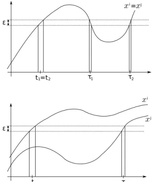
Let ε∈ R+and (x, y)∈(C0([0, T ]; X))n×(C0([0, T ]; Y))n
with X, Y two Banach spaces; we denote: Ωx,ε:= ∪ i,j=1:n{(i, j)} × Ω i,j x,ε, (52) where Ωi,j x,ε := { (t, τ )∈ [0, T ]2; xi(t)− xj(τ ) 6ε} (see
figure 1 for some examples).
6 In the case where n = 1, we have ψ
∂tX = ∂tψX = γψX+ X; so
the measurement noise is not amplified by the computation of ψ∂tX.
Fig. 1. Examples of (t, τ ) in Ωi,ix,ε (top) and in Ωi,jx,ε (bottom)
Definition 5. The ε-cancellation operator Dεis defined by:
(x, y)7→ Dε(x, y) : Ωx,ε → Y
(i, j, t, τ ) 7→ yi(t)− yj(τ ). (53)
Proposition 4. (1) Dε is continuous.
(2) For any continuous function f : X0⊂ X → Y, we have
the cancellation property:
D0(x, f◦ x) = 0. (54)
Thanks to proposition 4 and by application of operator D0(X, .) to both members of the equation, model (45) is
rewritten: { ⟨ µ, D0 ( X, ψ∂n tX )⟩ = D0(X, v) ⟨ µ, ψ∂n tX(0, .) ⟩ − f(X(0)) = v(0). (55)
The interest of this new formulation is that, on the one hand, up to the quantity f0 := f (X(0)), the model is
independent of f , and on the other hand, both µ and f0
are linearly involved. Formally, these unknowns can then be determined by means of the pseudo-inverse of operator:
Y0: (µ, f0)7→ ( ⟨ µ, D0(Xm, ψ∂n tXm) ⟩ ⟨ µ, ψ∂n tXm(0, .) ⟩ −f0 ) . (56)
In general however, on the one hand the set ΩXm,0 may
be too poor to get the strict equivalence of (45) and (55) and, on the other hand, the available data Xmand vmare
noisy. In practice, we so consider the weakened problem: min
(µ,f0)
∥ϵ(µ, f0)∥ 2
, (57)
where the equation error ϵ(µ, f0) is given by:
ϵ(µ, f0) =Yϵ(µ, f0)− ( Dε(Xm, vm) v(0) ) , (58) with: Yϵ: (µ, f0)7→ ( ⟨ µ, Dε(Xm, ψ∂n tXm) ⟩ ⟨ µ, ψ∂n tXm(0, .) ⟩ −f0 ) . (59)
The estimator (ˆµ, ˆf0) of (µ, f0) is then defined by: (ˆµ, ˆf0) =Yε† ( Dε(Xm, vm) vm(0) ) . (60)
By means of standard regression methods, the function f can then be easily estimated from its ”pseudo graph”:
Pf = ∪ k {( Xmk,⟨µ, ψˆ ∂n tXm(tk, .) ⟩ − vk m )} . (61)
The hypothesis made on f and n are more restrictive than those made for the method of simultaneous identification of f and H(∂t). Nevertheless, this method presents some interesting advantages. First, as the identification of f is uncoupled from the one of H(∂t), it is possible to adapt the choice of basis functions to the behavior of function f given by its pseudo-graph. Second, this method can also be used when the function f changes from one data set to the other. This identification method is still under study: more information about it will be found in (Casenave and Montseny [2009a]).
4.3 Iterative method
The identified quantities ˆµ and ˆf can be used as initial
values for an iterative identification method in order to improve the estimation quality. For example, let’s assume that the estimated operator ˆH(∂t) is exact; we can identify
the function f again, this time independently from H(∂t).
From the so-identified function denoted ˆf1, we identify
H(∂t), and we then reiterate until the quality of the
estimation becomes sufficient. Note that the convergence of such a method is still under study.
4.4 Identified model
The physical system under consideration can be de-scribed by the model H(∂ˆ t)X = f (u, X) + v whereˆ
ˆ
H and ˆf are deduced from the identified parameters.
Furthermore, by assuming that ˆH(∂t)−1 is γ-diffusive
of degree n′, we deduce from the equivalent expression
X = H(∂ˆ t)−1
( ˆ
f (u, X) + v
)
the following input-output state realization : ∂tψ = γ ψ + ˆf ( u, ⟨ (ˆµ)−1♯δn+n′, ψ ⟩) + v, ψ(0, .) = 0, X = ⟨ (ˆµ)−1♯δn+n′, ∂tn′ψ ⟩ , (62) which is available up to the computation of (ˆµ)−1♯δn+n′
which can be numerically performed as shown in (Casenave [2009]).
5. APPLICATION TO A MODEL OF FLAME In this section, we illustrate the identification methods presented above by implementing them on data elabo-rated from numerical simulations of a complex dynamic phenomenon (Joulin [1985]).
5.1 The model under consideration
In (Joulin [1985]), Joulin elaborated a Volterra model to describe, in suitable thermodynamic conditions, the
0 0.5 1 1.5 2 2.5 3 3.5 0 0.5 1 1.5 time t
(a) Source (- - -) and radius of the flame (—) with E = 1.7390.
0 1 2 3 4 5 6 7 0 1 2 3 4 5 6 7 time t
(b) Source (- - -) and radius of the flame (—) with E = 1.7393.
0 1 2 3 4 5 6 0 2 4 6 8 10 12 time (s)
(c) Trajectories X used for identification.
Fig. 2.
evolution of a spherical flame initiated by a source at point 0 in a mixture of reactive species. Under some reasonable physical hypothesis, such a phenomenon can be described by a system of two partial differential equations relating to the temperature and the mass density of the mixture. By considering the reactive zone as a thin sheet located on a sphere with radius X(t), Joulin has established that when the flame is developing in free space, X is solution of the following nonlinear singular Abel-Volterra equation7
(e(t) designates the source strength at time t):
X(t)∂
1 2
t = 2 X(t) ln X(t) + 2 e(t) ∀t > 0, (63)
with the additional conditions: X(0) = 0, e> 0, X > 0 (whose physical interpretation is obvious). By denoting
H(∂t) = 12∂ 1 2 t, f (u, X) := ln X = f (X) and u = e X, (63)
can be formally rewritten under the form (45). We have:
• H(p) p = 1 2p− 1 2 holomorphic inC r R−, • and H(p) p → 0 when |p| → 0 in C r R−;
so H(∂t) is γ-diffusive of degree 1 for any γ of the sector
form (44).
As shown in (Audounet et al. [1998]), the evolution prob-lem (63) is well-posed, that is the solution X exists, is unique and depends continuously on e. It has also been shown that there exists a threshold relating to the power of the source e, beyond which the flame is developing whereas a quenching occurs below, as it is highlighted in Fig 2a and 2b, the source function used for the simulation being given as in (Audounet et al. [1998] by:
e(t) = E t0.3(1− t) 1[0,1](t). (64)
In real conditions, various perturbations are involved in the evolution of X (due for example to the loss of spatial symmetries), and both the convolution operator H(∂t) and
the function f will be more or less far from the ideal ones. So, an identification process can be justified if accuracy of the model is required.
5.2 Numerical identification results and comments
We consider in the sequel the problem of identification of
H(∂t) and/or f from data (em, Xm) obtained from highly
accurate numerical simulations of (63) (Montseny [2010]). The data are composed of 9 discrete simulated trajectories (ej,k
m , Xmj,k)k=0:K, j = 1 : 9 (see figure 2c), associated
with 9 different sources ej of the form8 (64) with E = 1.5, 1.6, 1.7, 1.73, 1.74, 1.75, 2.0, 3.0 and 5.0 respectively. The time step ∆t is constant and equals to 10−5 and the final time is given by tK= 6 (K = 6× 10⁵).
The inputs are supposed to be known:
ej,km = e
j
(tk), (65)
and the outputs are corrupted by additive measurement noise:
Xmj,k= Xj(tk) + vj,k, (66)
where {vj,k} is a numerical white noise with zero mean
and of standard deviation s = 10−1.
To identify H(∂t), we use L = 80 values ξlL geometrically
spaced to cover 5 decades from 100to 105, and we consider a contour γ of the form (44) with α = π4. To identify f , we use 30 basis functions kq, q = 1 : 30, of hat type and
one function basis g1= 1.
The frequency response of the identified operator ˆH(∂t)
and the curve of the identified function ˆf are given in
figure 3 when f is supposed to be known (see section 3), when f and H(∂t) are simultaneously identified (see
section 4.1) and when H(∂t) is first identified alone after
cancellation of f (see section 4.2). For the 3 methods, the identification of H(∂t) is good in the frequency band
[100, 102] ⊂ [K ∆t2 π ,2 ∆t2 π] = [1.05, 3.14 105] (in the free noise case, this frequency band covers 4 decades). The identification of f is also good, even around the singularity of the function f at X = 0. Note however that the greater
8 Note that the source function is physically realistic but rather poor
from the point of view of information, which strengthen the difficulty of the problem. 10−2 10−1 100 101 102 103 104 105 −50 −30 −10 10 30 50 pulsation ω (rad.s−1) magnitude (dB) 10−2 10−1 100 101 102 103 104 105 −180° −90° 0° 90° 180° pulsation ω (rad.s−1) phase (degree) 0 1 2 3 4 5 6 −7 −6 −5 −4 −3 −2 −1 0 1 2 X function f simultaneous identification theoretical
identification when f is known identification after cancellation of f
simultaneous identification theoretical
identification after cancellation of f
Fig. 3. Identification results.
the value of X is, the larger the difference between f (X) and its estimate ˆf (X) is; this is partly due to the fact that
there are more data Xj,k
m with value near from zero than
others.
6. CONCLUSION
In this paper, we have shown how to use the diffusive representation in order to identify the dynamic part of a system. Thanks of the linearity of the γ-symbol in the state realization of the operator H(∂t), we can identify
it by means of classical least squares methods. Several questions must yet be studied in order to improve the results. For example, among the most significant, the involved hilbertian norms should be judiciously chosen and adapted to the specific properties of the class of models under consideration; indeed, this choice is crucial in terms of sensitivity with respect to perturbations of any nature. The estimation bias could also be reduced. All these questions are currently under study.
REFERENCES
Audounet, J., Giovangigli, V., and Roquejoffre, J. (1998). A threshold phenomenon in the propagation of a point source initiated flame. Physica D: Nonlinear
Phenom-ena, 121(3-4), 295–316.
Ben-Israel, A. and Greville, T. (2003). Generalized in-verses: Theory and applications. Springer Verlag, New
York, USA.
Carmona, P. and Coutin, L. (1998). Fractional brownian motion and the markov property. Electronic
Communi-cations in Probability, 3, 95–107.
Casenave, C. (2009). Repr´esentation diffusive et inversion op´eratorielle pour l’analyse et la r´esolution de probl`emes dynamiques non locaux. Ph.D. thesis, Universit´e Paul Sabatier, Toulouse.
Casenave, C. and Montseny, G. (2008). Identification of Nonlinear Volterra Models by means of Diffusive Representation. In 17th IFAC World Congress, 4024– 4029. Seoul (Korea).
Casenave, C. and Montseny, G. (2009a). Diffusive Iden-tification of Volterra Models by Cancellation of the Nonlinear Term. In 15th IFAC Symposium on System
Identification, SYSID 2009. Saint-Malo (France).
Casenave, C. and Montseny, G. (2009b). Optimal Iden-tification of Delay-Diffusive Operators and Application to the Acoustic Impedance of Absorbent Materials. In
Topics in Time Delay Systems: Analysis, Algorithms and Control, volume 388, 315. Springer Verlag, Lecture
Notes in Control and Information Science (LNCIS). Casenave, C. and Montseny, G. (2010). Identification and
State Realization of Non-Rational Convolutive Models by Means of Diffusive Representation. Submitted to IET
Control Theory & Applications.
Degerli, Y., Lavernhe, F., Magnan, P., and Farre, J. (Ap. 1999). Bandlimited 1/fα noise source. Electronics
Letters, 35(7), 521–522.
Garcia, G. and Bernussou, J. (1998). Identification of the dynamics of a lead acid battery by a diffusive model.
European Series on Applied and Industrial Mathematics (ESAIM): Proceedings, 5, 87–98.
Joulin, G. (1985). Point-source initiation of lean spherical flames of light reactants: an asymptotic theory.
Com-bustion science and technology, 43(1-2), 99–113.
Lenczner, M. and Montseny, G. (2005). Diffusive realiza-tion of operator solurealiza-tions of certain operarealiza-tional partial differential equations. CRAS - Math´ematiques, 341(12),
737–740.
Levadoux, D. and Montseny, G. (2003). Diffusive formula-tion of the impedance operator on circular boundary for 2D wave equation. In The Sixth International
Confer-ence on Mathematical and Numerical Aspects of Wave Propagation. Jyv¨askyl¨a (Finland).
Monin, A. and Salut, G. (1996). ARMA lattice identifi-cation: a new hereditary algorithm. IEEE Transactions
on Signal Processing, 44(2), 360–370.
Montseny, E. (2010). Desingularization of non local dy-namic models by means of operatorial transformations and application to a spherical flame model. Submitted to
4th IFAC Symposium on System, Structure and Control.
Montseny, G. (2005). Repr´esentation diffusive. Hermes
Science Publ.
Montseny, G. (2007). Diffusive representation for oper-ators involving delays. In Applications of Time-delay
Systems, 217–232. Springer Verlag, Lecture Notes in
Control and Information Science (LNCIS).
Montseny, G. (Nov. 2004). Simple approach to approxi-mation and dynamical realization of pseudodifferential time-operators such as fractional ones. IEEE Trans on
Circuits and System II, 51(11), 613–618.
Mouyon, P. and Imbert, N. (2002). Identification of a 2d turbulent wind spectrum. In Aerospace Science and
Technology, volume 6, 3599–605. Kansas City (USA).
Rumeau, A., Bidan, P., Lebey, T., Marchin, L., Barbier, B., and Guillemet, S. (2006). Behavior modeling of a cacu3ti4o12 ceramic for capacitor applications. In
IEEE Conference on Electrical Insulation and Dielectric Phenomena. Kansas City (Missouri USA).