February 1978 ESL-P-799
CERTAINTY EQUIVALENT SOLUTIONS OF QUADRATIC TEAM PROBLEMS BY A DECENTRALIZED INNOVATIONS APPROACH*
by
Steven M. Barta** Nils R. Sandell', Jr.-***
-Abstract
This paper considers a team decision problem with a quadratic loss function. It is shown that the optimal solution satisfies a certainty equivalence type separation theorem. When the state and the agents' information vari-ables are continuous-time stochastic processes, the solution to the estima-tion part of the decision rule is characterized by an integral equaestima-tion. By introducing a decentralized innovations process, this equation is solved. If the state is generated by a finite-dimensional linear system and each agent has a (possibly) distinct linear noise corrupted observation of the state, then the optimal decision rules are generated recursively from a decentralized linear filter. Also, a second-guessing paradox is resolved.
*Research supported by the National Science Foundation under grant NSF/ENG-77-19971 and by the Department of Energy under grant ERDA-E(49-18)-2087. **Room 35-437, Electronic Systems Laboratory, M.I.T., Cambridge, Mass. 02139
The optimal actions in a general stochastic control problem serve the dual functions of estimating unknown states of the system and of guiding
the system to achieve desired performance.l When it is possible to divide ex-plicitly the optimal control law into an estimation part and a decision part, the law obeys a separation principle. The best known example of such a
result is the optimal solution to the Linear-Quadratic-Gaussian (LQG) problem with classical information pattern.
Though in many cases it is difficult to compute the optimal control even if it satisfies a separation theorem, the structural insight gained from a separation result is valuable in designing a suboptimal controller. In particular, estimation and decision schemes might be designed independently and then combined to form a reasonable overall control law. Moreover, if the estimation problem is solved by a finite-dimensional sufficient statistic which may be updated recursively, then large scale data reduction is possible.
The Kalman filter estimate, for example, is a sufficient statistic for the LQG problem with classical information pattern. Thus, although the optimal
trol law is a functional of all past data, the information necessary for con-trol is summarized in the estimate.
There have been several generalizations of the LQG result, but most 2
attention has been focused on classical information patterns. Though dynamic systems are often accurately described by classical information patterns, in many situations decision-making is decentralized among several agentseach of whom acts on the basis of different information. These decentralized systems
1
See Fel'dbaum [6] for a pioneering treatment of the dual effect. For more recent results, see Aoki [1] and Bar-Shalom and Tse [4].
2
-2-have nonclassical information patterns . When agents have a common objective, we have a team decision problem. For dynamic teams, optimal recursive
solutions have been determined only in a few cases. Sandell and Athans [16] present a recursive solution for the 1-step delay problem and discuss control sharing information patterns. Kurtaran and Sivan [11] and Yoshikawa (21]
also solve the 1-step delay problem.
One-step delay problems are examples of systems with partially nested information.5 Ho and Chu [7] prove that if the state of a partially nested system has linear dynamics, if the criterion is quadratic, and if all random variables are Guassian, then the optimal solution is a linear function of the observations. It is not known, however, for which partially nested sys-tems separation principles hold nor which syssys-tems admit recursively generated sufficient statistics.
In this paper we study the optimal solutions for a class of team decision problems with a criterion which is a quadratic function of the decisions and of a random variable called the state. The state and information variables are unaffected by the decisions, and, therefore, these systems are a subset of the class of partially nested systems.
In Section II, we prove the optimal solution may be separated into an estimation part and a decision part. The estimates form a set of sufficient statistics for a set of problems in the sense that, under decentralized
3
See Radner [14] and Marschak and Radner [13] for an introductory discussion of the static case. Witsenhausen [18,191 and Ho and Chu [7] consider
dynamic problems. 4
In several other decentralized problems, as in for example Chong and Athans [ 5], solutions have been found which were a priori restricted to be recursive. In general these solutions are suboptimal with respect to
classes of control laws which include nonrecursive schemes. In this paper, optimal recursive solution means there does not exist a nonrecursive solution w'hich improves performance.
5If a decentralized problem has partially nested information, then control actions propagate at a rate no greater than information. Therefore, there is no need to communicate information through the controls. See Ho and Chu-[7].
information, these estimates are inserted where the known state appears in
the optimal decision rule under complete information, i.e. under certainty.
Thus, we have a certainty equivalence separation theorem. In this section
we also introduce a matrix notation to emphasize the parallelism between
this team problem and classical quadratic loss decision theory, and we
characterize the estimate in terms of an orthogonal projection.
Section III considers the same objective function as in II, but here we
impose an explicit temporal structure by assuming the state and information
variables are continuous-time stochastic processes. The orthogonal projection
characterization of the optimal linear solution yields an integral equation
which we call the decentralized Wiener-Hopf equation. By generalizing the
classical linear innovations theorem, we solve the equation. When all random
variables are Gaussian, we prove our solution is optimal over the class of
all (linear and nonlinear) causal functionals.
In Section IV, we specialize to the case where the state is generated
by a finite-dimensional linear system and the observations are linear in the
state.
Here the team estimates are generated from a set of finite-dimensional
recursive equations reminiscent of the Kalman-Bucy filter.
Section V contains the
conclusion.-Notation:
(a) If P. (i=l), ,,,fN1
iS an mi.
x n matrix, then let
-4-P1
0
diag [P1,i .. PN ]
0 PN
be a matrix with blocks P. on the diagonal and the 0 matrices chosen so that N
diag[P1 ... ,PN] is MXnN, where E mi M. i=l
(b) If EJxl2 < o for a random variable x, then x is a second-order random variable. A second-order process {x(T), 0 < T < T is such that x(T) is a second-order random variable for all T E [0,T]. All processes and random variables in this paper are assumed to be second-order, unless we specify
II. Static Quadratic Teams
In the quadratic team decision problem, there are several agents or decision-makers each of whom selects a control action as a function of the available information so that the expected value of a quadratic function is minimized. The situation is static when no explicit temporal ordering is imposed on either the decision or the information variables. To make these informal remarks precise, define a probability space (Q,~,~). The team problem is to minimize the Bayes loss
Jl(U) = E[(u-Lx)' Q -Lx)], (1)
where Q = Q'> 0 is an MXM matrix, x is an n-dimensional random vector, L is an Mxn matrix, u is a vector composed of M scalar components u.; and the expectation is taken with respect to the probability measure If. The compon-ents u. of the decision vector are restricted to be functions of a set of measurable information functions Yi. :Q Si, where Si is a vector space. Si might, for example, be Rm or if the information is a stochastic process, it may be L2 [O,T]
m
. Equivalently, we may say u. is S.-measurable, where i is
1 1
the sigma-field generated by Yi. Note that Yi - Y i4j,is not excluded.
The interpretation of this is simply that some agents may make vector- decisions. The problem of minimizing (1) is basically the problem treated by Radner [14]. To derive a certainty equivalent solution and a set of sufficient statistics, we consider a slightly more general problem. Define the nMXM partitioned matrices d1 D L (2)
LdM_
and X E diag [x, ..., x], (3) 6-6-where d. is an nxM matrix and column i (i=l,...,M) of D is restricted to be a
1
function of Yi.
Now let the team loss function be
J
2(D)
=
tr E[(D-X)Q(D-X) ]
(4)
where tr is the trace operator. By writing out (4), we find that row (j(j=l,...,n)
of block i(i=l,...,M) is the matrix D corresponds to the decision vector u in a
team problem of the form min Jl(u), where L has a 1 in element (i,j) and zero
elsewhere.
Thus minimizing J
2(D) is equivalent to solving nM separate team
problems of the form min Jl(u).
The reason problems of the form min J
1(u) may
be solved by solving min J
2(D) is that u-LX is linear in L and the solution for
any L is expressed in terms of a set of basic solutions which are contained in
the optimal matrix D. See Theorems 2 and 3 below.
We have introduced J
2(D) because it allows us to draw a clear parallel
between classical and nonclassical quadratic loss decision theory. In particular.
the idea of certainty equivalent decision rules as functions of a set of
sufficient statistics appears naturally (Theorem 2 below) in this formulation.
To characterize the solution to (4), we develop the following vector
space interpretation.
Let 'be the space of all nMXM matrices whose elements
are measurable functions from Q to R
,
i.e. scalar random variables.
Define
<H
1,
H
2> -
trE [H
1QH
2](5)
for Hi EgXand note that (5) is well-defined since we assumed all random
vari-ables are second-order.
It is routine to verify that with inner product (5)
and norm
11H11
2=
<H,H
>,
lpisa Hilbert space.
Let ~ be the subspace of all D sC withcolumn i dependent only on Yi.
By the Hilbert space projection theorem [Luenberger [12], p. 51], we have
the following result characterizing the nMXM matrix X
E!
which solves
min J
2(D)
.
Theorem 1:
The minimum of < D- X, D- X > for D 6E is achieved
by the unique X $ satisfying
<X-X,D > -
trE[(X-X)QD'] = 0,
(6)
Next, letdA be the subspace of ! in which the elements of D are restricted to be affine functions of the Yi. Then Theorem 1 also holds with f replacing
gand we call the X which minimizes (4) overe,a, the optimal linear solution. Condition (6) is a generalization of the classical orthogonality con-dition that defines the concon-ditional expectation and the linear regression estimate, respectively, in the cases where the estimate is unconstrained or constrained to be linear. Note that, unlike the classical case, the estimate depends on Q.
Condition (6) also implies a further useful characterization of the optimal decisions. Because KD E I for any real nMXnM matrix K, (6) implies
< (X-X),KD> = 0 (7)
for all D E£. Therefore definition (5) and (7) give
trE [(X-X)Q(KD)'] = trE [K' (X-X)QD'] = O , (8) where the first equality is a property of the trace operator. Since (8) is
true for all real K, we have
E[(X-X)QD'] =
0
(9)for D £I.
If we interpret X as a team estimate of X, we may prove a certainty equivalence theorem.
Theorem 2: Let ~ be an nMXnM matrix. Then the optimal solution to the team problem
min < D - (X, D- NX > , (10)
where D CE and X is defined by (3) is (X, where X solves min [J2 (D) ID S].
Proof: A necessary and sufficient condition that D* solves (10)is
< D* - (X, D > = 0 (11)
To see that Theorem 2 is a certainty equivalence result, simply note that if X assumes a single value, say Xo, with probability one, then fXo solves
(10). Thus, this theorem generalizes the certainty equivalence result of classical decision theory which states the solution of the quadratic loss problem min.E[(u-Gx)'(u-Gx)],where xis a random vector and u is the decision, is Gx, where x solves the estimation problem min E[(u-x)'(u-x)].
Theorem 2 also allows us to solve the original team problem with criterion J (u).
Theorem 3: Let L. be row j of the matrix L. Then the optimal J
solution u* to min Jl(u) is
u.* = Lx., (i=l, ...,M), (12)
I
j=l 1
where A. is column i of X. (Note: x.. is an n-vector.) j31
XMi Proof: Setting
pL
[Li,
-- , LjM (13)L
L
0in (10) yields the objective
nM
< D- 0LX, D - (LX>
=E[(D
l-(Lx)')Q(D-Lx) +
D
D.Q!D,
(14)
i=2where Di is row i of D. The first term on the right-hand side in (14) is Ji(D'). By Theorem 2 the solution D* minimizing (14) is
D*
LX
=[
0 (15)where u* is as defined in (12). Q.E.D.
It is important to note that although we have a certainty equivalent solution for min J2 (D) if U solves the team problem min E [ (u-x) 'Q(u-x)] , then in general the optimal solution to min Jl(u) is not Lu.
III. Stochastic State and Information Processes
In this section we discuss a stochastic process version of the team problem with
objective (1), i.e. let the objective be
Jl(u(t)) = E[(u(t) - L(t)x(t))'Q(u(t) - L(t)x(t))], (16)
where Q = Q'> 0 , {x(T), 0 <
T< T} is a zero-mean n-dimensional state process,
L(t) is an MXn time-varying matrix, and {u(T), 0 < T < T} is a decision
pro-cess whose components u.
(-) are restricted to be causal linear functions of
a zero-mean pi-dimensional observation process {yiT), 0 <
T< T}.
7This is
a team analogue of classical linear quadratic dynamic decision theory.
The results of Section II imply that we solve (16) by a separation
principle, i.e. by first solving the estimation problem (which is independent
of L(t)) of minimizing
J2(D(t)) = trE[(D(t) - X(t))Q(D(t) - X(t))'], (17)
where X(t) - diag [x(t), ...,x(t)], and column i (i=l,...,M) of D(t) is
restricted to be a causal linear function of y i
(-)),
and then applying Theorems
2 and 3. Note that (17) is not really more general than the problem in
Section II.
In this section we are solving a series of problems of the form
(10) on the interval [O,T] and imposing a specific stochastic process
structure on the general information spaces of Section II.
Because the decision at time t must be a linear function of
{yi()
, 0
< T <t}, column i of the optimal decision X(t), x (t), may be
written
4i
t
x (t)
=
0
Hi
(t,T)
yi() dT,
(18)
where Hi(t,T) is an nMxpi matrix. Thus, we have
t
X(t) =
f
H(t,T)Y(T)dT ,
(19)
0
7
There is really no loss of generality in restricting these processes to be
zero-mean.
A nonzero mean will simply add a constant term to the optimal
decisions.
-10-where H(t,T) - [Hl(t,T), ..., HM(t,T)] and the PXM partitioned matrix Y(T) is defined as
Y(T) - diag [y1(T) ... YM (20)
M and P- Pi.
i-1
To find H(t,T), we use the criterion (6). In this case X(t) - X(t) must be orthogonal to all linear function of the data satisfying the information constraints. Hence, the error must be orthogonal to all individual terms of the form KY(s), 0 <s <t, where K is a real nMXP matrix. As in (9), this gives
E[(X(t) - X(t))QY'(s)] = 0, 0 < s < t. (21) Defining the notation
E[Y(t)QY' (s)] - y (t,s) (22)
E[X(t)QY'(s)] - ZY (ts) (23)
and substituting into (21) yields E[ t H(t,T)Y(T)OY' (s)dT] =
ft H(t,T) 7 (T,s)dT = (t,s). (24)
0O YY;Q XY;Q
Equation (24) is a nonclassical version of the nonstationary Wiener-Hopf equation. For the same reasons as in the classical case, this equation is hard to solve. For certain special cases, however, the solution to the classical Wiener-Hopf equation is very easy to find. For example, if the
observation process is white noise, then there is a simple formula forthe
opti-mal estimating filter. Sometimes it is possible to replace the observations
by a related white noise process that is equivalent to the original process in
the sense that estimation performance remains unchanged if the new process is
used to compute the estimate. The related process is called the innovations
We will develop a decentralized innovations method to solve (24) and to
do this we need an extended definition of white noise process.
Definition 1:
Let {V(T), 0
<
T<
T} be an NXM matrix
process. Then V(-) is a Q-white noise if and only if
E[V(t)QV' (s)] = Z (t) 6(t-s) , where Z (t) > 0.VV;Q
VV;Q
-Remark:
Definition 1 is a nonrigorous definition as is the classical white
noise definition. Tobe rigorous we define the integral M'(t) - f0
tV(T)dT as a
Q-orthogonal increments process, i.e.
E[1/(t)Q/''(s)] = tA
sV
(T)dT
,(25)
where tAs - min(t,s). Although the subsequent arguments in this paper are
in terms of the Q-white noise, everything may be made rigorous by working
with Q-orthogonal increments processes.
Next, we prove that if the team information is a Q-white noise, then (24)
is easy to solve. Let the team information process be the Q-white noise
process V(-) where column i of V(.) is team member i's information. Then let
the optimal solution be
X(t) =
J
tG(t,T)V(T)dT. (26)
Remark:
Because Y(T) has the form (20), expression (19) is equivalent
to (18), i.e. it represents all linear functions of the data. Also because
V(-) is not necessarily of the form (20), (26) is not the most general linear
function such that column i of X(t) is only a function of the elements of
column i of V(-).
For our purposes, however, (see Theorem 4, below), (26) is
sufficiently general.
As in (24), we derive
E[ f0t G(t,T)V(T)QV' (s)dT] = G(t,s) Z W; Q(S) = XV;Q(t,s), (27)
See Kailath [8,9] for several discussions of innovations processes,
applica-tions, and references to other work.
-12-where the first equality holds because V(-) is a Q-white noise. Therefore if VV;Q(t) is nonsingular, then
G(t,s) = ;Q(t,s) ;Q(S)
XV;Q VV;Q
and
X(t)
=fV
() (tT) Z (T))V(T)d. (28)This formula resembles the classical linear least squares result except that our V(-) is a Q-white noise process and the solution is the matrix X(t) rather than a vector. Note also the integrand of (28) is a function only of a priori information, and column i of X(t) is a function only of
column i of {V(T), 0 < T < t} as is required in the team problem.
Although (28) is a useful formula when the information is a Q-white noise process, in most cases it will not have this property. In some models the observations are equivalent, however, to a Q-white noise process in the sense that any linear function of the original observations may be written as a linear function of the related process. We call the related process a non-classical innovations process. In addition, this process may be obtained by passing the observations through a causal and causally invertible decentralized filter. In the decentralized filter, each agent of the team puts his own ob-servations into a causal and causally invertible filter. Then the individual output processes form the columns of the nonclassical innovations process, which satisfies Definition 1.
In classical theory, the observations are often assumed to have the form
y(t)
-
z(t) +
e(t),
0
< t < T,
(29)
where E[e(t)e' (s)] = 6(t-s), E[z(t)z'(t)] <00, and past signal is uncorrelated with future noise, i.e.
E[O(t)z'(s)] = 0, O < s < t < T. (30) To derive a nonclassical analogue of (29), let Ci(t) (i=l,...,M) be a
Pixn matrix and define the PXM matrix
Xc(t) = C(t)X(t),
(31)
M
where P -
; Pi, C(t) - diag[Cl(t),...,CM(t)],
and X(t) is defined as in (17).
i=lAlso define the PxM matrix process
0(t)
- diag[(t) , ... , (t) (32)where e (t) is a pi-dimensional process and
E[Q(t)QO' (s)] =
G
;Q(t) 6(t-s) , ;Q(t)>
0f 0 < t,s < T. (33)Now let the team observation matrix Y(t) satisfy
9Y(t) = Xc(t) + O(t),
(34)
and assume future values of
0(-)
are Q-orthogonal to past values of Xc(-), i.e.
E
[O(t)QXc (s)] = 0,
< s < t < T.
(35)
The interpretation of (34) is that team member i observes a noise corrupted
measurement of linear combinations of the state vector x(.).
Thus, (34) is
equal to
Yi(t) = Ci(t)x(t) +
eO(t),
i=l,...,M.
(36)
Let the team estimate of Xc(t) given the information {Y(T), 0 <
T <t}
be denoted Xc(t).
Theorem 2 implies Xc(t) = C(t)X(t), where X(t) is the
optimal linear estimate of X(t).
Therefore,
Xc (t) = C(t)
f
tH(t,T)Y(T)dT
C
0
-t R(t,T)Y(T)dT, (37)
where H(t,T) is defined by (24).
We now define a nonclassical innovations
process.
See also (I.4), in Appendix I, the equation for R(t,T).
Definition 2:
The nonclassical innovations process for the team
problem of minimizing J
2(D(t)) with data (34) is the process
9
Note that it is possible to have a Z(t) process in (34) instead of X (t),
c
where Z(t) is related to the state process.
For our purposes, however, we
do not need this slightly more general formulation.
A sufficient condition for (35) is that future values of ei(.) (i=l,...,M),
are uncorrelated with past values of x(-).
-14-V(t) = Y(t) - Xc(t)
= C(t)(X(t)-X(t)) + 0(t)
(38)
The following theorem is a nonclassical version of the linear innovations
theorem.
Theorem 4:
The innovations process, defined by (38) satisfies the
following properties.
(i) E[V(t)QV'(s)] = E; Q(t) 6(t-s),
(39)
where e Q(t) is defined in (33).
(ii) Z{v(T), 0 < T < t} = Z{Y(T), 0 < T < t},
(40)
where for a matrix process M(-), Z{M(T), 0 <
T
< t} is the set
of linear functions of the formft
N(t,T)M(T)dT , for somematrix kernel N(t,T).
Proof:
Appendix I.
Condition (i) of the theorem says V(-) is a Q-white noise with the same
Q-covariance as the process noise
0(t).
Condition (ii) says that any linear
function of the observation process may also be written as a linear function
of the innovations. The reason for this is that the operator R whose kernel
is defined by (37) is causal and causally invertible, i.e. if we write in
operator notation
V = (I-R)Y, (41)
-1
then (I-R)
is causal and
-1Y = (I-R)
V .
(42)
Figure 1 illustrates the structure of the optimal solution D*(t) of the
problem of minimizing <D(t) -
¢(t)X(t), D(t) - 0(t)X(t)>.
Of course, Figure
1 is equivalent to M separate structures, each computing a column of X(t),
as is required by the decentralized information constraint. Moreover, it is
crucial to remember that to simplify the solution to the decentralized
Wiener-Hopf equation, it is not sufficient for each team member to whiten his own
l (t
Figure 1. The optimal linear team decision structure.
observation process, i.e. to compute
Vi. (t) = Yi(t) - C. i(t)(t), (43)
where x(t) is the classical linear least-squares estimate based on Yi(.); the matrix process V(-) - diag[Vl(' ),... vM( )] is not a Q-white noise. But rather a joint whitening of the aggregate information process Y(t) must be carried out within a decentralized computational scheme.
The final topic of this section is a proof that when the state and infor-mation processes are all jointly Gaussian, the optimal linear causal solution is optimal over the class of all (linear and nonlinear) causal solutions. To prove this let D(t) - D[Y(T), 0 < T < t] be an arbitrary causal function of
the data with column i of D(t) only a function of {yi(T), 0 < T < t}. We will show J2(D(t)) > J2(X(t)), where X(t) is the optimal linear estimate. Begin by writing
-15-t G(-15-t,'r)V(T)d'T
t
0(t)
Figure 1. The optimal linear tea= decision structure.
observation process, i.e. to compute
1 1 3.
vi(t) = Yi(t) - Ci(t)x(t), 4
where ~(t) is the classical linear least-scuares estimate based on yi(.); the matrix process V(') - diag[vl(),...,v~M(-)] is not a Q-white noise. But rather a joint whitening of the aggregate inforation process Y(t) must be carried out within a decentralized computatic-nal scheme.
The final topic of this section is a prcof that when the state and infor-mation processes are all jointly Gaussian, the ori.al linear causal solution
is optimal over the class of all (linear and nonlinear) causal solutions. To prove this let D(t) _ D[Y(T), 0 < T < t] be an ar-_trary causal function of
the data with column i of D(t) only a functic-n of {v. () , 0 < T < t}. We will show J2(D(t)) > J2 (X(t)) , where X(t) is the tirl linear estimate. Begin by writing
J2(D(t)) - tr E[(D(t) - X(t)) Q(D(t) - X(t))'] = tr E[(D(t) - t) +X(t) - X(t)) Q(D(t) - X(t) + X(t) - X(t))'] = tr E[(D(t) - X(t)) Q(D(t) - X(t))' + 2(X(t) - X(t)) Q(D(t) - X(t))'] + J2(X(t)). (44) To prove E[(X(t) - X(t)) Q(D(t) - X(t))'] = 0 (45)
first note the orthogonality condition (21) implies
E[(X(t) - X(t)) QX•' (t)] = 0. (46)
Second, (21) and the Gaussian assumption imply each component of the vector process {yi(T), 0 < T <
t}
is independent of all elements of column i of the matrix (X(t) - X(t))Q. Therefore,E[(X(t) - X(t))QD' (t) = 0 (47)
and
J2(D(t)) = < D(t) - X(t), D(t) - X(t) > + J2 (X(t)) > J2 (X(t)). (48)
-17-IV. The Decentralized Kalman-Bucy Problem
By assuming X(t) solves a finite-dimensional linear stochastic differ-ential equation, we derive a recursive formula for the team estimate X(t). Let x(t) solve the equation
x(t) = A(t)x(t) + W(t),
x(O) = x,, 0 < t < T, (49)
and E(t) satisfies
E[E(t)] = 0, E[E(t)' (s)] = 7 (t) 6(t-s)
z (t) > 0 0 < t,s < T, (50)
and
Ex0 = 0, Ex0x = > 0, E[(t)x] = 0 (51)
To put this into partitioned matrix form, define
jI(t)
- diag [A(t),..., A(t)] (52)E(t) - diag [~(t),..., ~(t)] (53)
whered(t) and E(t) each have M blocks. Then we have X(t) ='4(t)X(t) + F(t) X(O) = XG, 0 < t < T, (54) and E[5(t)] = 0, E[((t)QH'(s)] = 7 (t)
S(t-s)
= = (Q®I)diag[EZ(t),..,,7Z(t)] 6(t-s), (55) and EX0 = 0, E[3(t)QXO] = 0,E[XoQX' ] X = = Q®I diag[E ] 7 (56)
xax0;Q x0 x-0 ,- , - xx
where the Kronecker product Q0I satisfies
qll I qlMI
QI- .
(57) qMnlI .. qMMI
The observations of team member i are
Yi(t) = Ci(t)x(t) +
ei(t),
(58)where C (t) is a pixn matrix and .(t) is a classical white noise satisfying
E[0i(t)) = 0, E[l
i (t) 6
(t-s)
ie e (t) > 0, E[(i(t)xO] = 0, E[0i(t)'(s)] =
.
(59) In partitioned matrix form, we haveY(t) = C(t)X(t) + (t), < t < T,
(60)
where C(t) - diag[Cl(t),...,CM(t)] and O(t) - diag[e1(t),...,EM(t)]. The assumptions on 8i(') imply 0(.) is a Q-white noise andE[O(t)] = 0, E[0(t)QO'(s)] = % Q(t) 6(t-s),
E[O(t)QX']
=0O
(61)
where Z:C;Q(t) = | qll 0 1 1 1M 01 M (62) 'Ct)~~~(62)
'IMl00 1%MM
OM
and Z Q(t) > 0 because Q > 0 and (59). Furthermore our assumptions also give
E[o(t)QX' (s)] = 0, 0 < s < t < T, (63) which is required in our innovations theorem.
To derive a recursive formula for X(t), we compute first the nonclassi-cal innovations process and then use formula (28) to find the decentralized filter. The innovations process is
V(t) = Y(t) - C(t)X(t)
= C(t)X(t) + 0(t), (64)
where
(t)
E X(t)
-
-(t)t). The result is contained in the next theorem.
X(t)
Theorem 5:
Let X(t) and V(t) satisfy (54) and (64) respectively.
Define
K(t) E (t)C' t) - (t) (65)
-19-and
E
(t) -E[X(t)QX' (t)].
(66)
Then the optimal linear team decision for (17) satisfies
X(t) =_4(t)X(t) + K(t)V(t), X(O) = 0, (67)
or equivalently, the optimal decision of agent i, i.e. column
i of X(t), satisfies
'i^i i
x (t) =d(t)x (t) + K(t)[Niyi(t)- C(t)x (t)i, (68)
M
where N = [O,...,I',...,0']' is a
P
Xp-dimensional
partitioned matrix with block j (j/i) a zero matrix with pj
rows and block i a p.-dimensional identity. Also E(t) solves
the Riccati equation
}(t) = (t)Z (t) + (t)' (t) -K(t)t ®; Q(t)K' (t)+ ;Q(t) ,
.(0) = X (69)
Proof:
For this problem (28) implies
A
-l
(70)
X(t) = t E[X(t)QV(T)] Q()V(T)d. (70)
Differentiating (70) and using (54), we obtain
A~
~~_-1
X(t) = E[X(t)QV(t)] 'Li (t) V(t)+
t E[X(t)QV(T)]E
-1(T)V(T)dT0
-1 = E[X(t)QV(t)] E3 Q(t) V(t) +,d(t)o0t E[X(t)QV(T)] Q(t)V;(T)dT +f0t
E[E(t)QV(T)] ]- (T) V(T) dT (71)The second term on the right-hand side of the second equality is4(t)X(t)
and the last term is zero by the assumptions (59) and
C(-)
is a white process.
For the first term we have
This proof is very similar to the derivation of the classical Kalman-Bucy
filter by the innovations method. See Kailath [8].
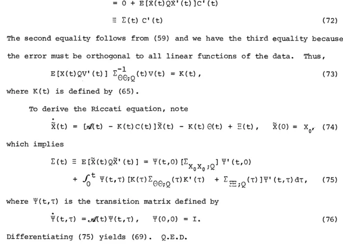
E[X(t)QV' (t)] = E[X(t)Q(X(t)C(t) + G(t))']
= E[(X(t) + X(t))Q(t)t)]C'(t) + 0 = 0 + E[X(t)Q'(t)Q C'(t)-- (t) C' (t) (72)
The second equality follows from (59) and we have the third equality because the error must be orthogonal to all linear functions of the data. Thus,
E [X(t)QV' (t)] _ Q(t)V(t) = K(t), (73)
where K(t) is defined by (65).
To derive the Riccati equation, note
X(t) = [d(t) - K(t)C(t) ]X(t) - K(t)
0(t)
+ (t), X(0) = X,- (74) which impliesE(t) - E[X(t)QX'(t)]
=
(t,0) X
;Q
i
'(t,O)
+
ft
T(t,T) [K(T)Z ;Q(T)K'()
+ + ;(T) ]T'(t,T)dt, (75)0 0- 0 ; ; Q
where T(t,T) is the transition matrix defined by
'P(t,T) =
d(t)T(t,T)
,
T(0,0)= I.
(76)
Differentiating (75) yields (69). Q.E.D.
Figure 2 illustrates the feedback structure of decentralized optimal filter. A striking feature of the filter is that all the agents' linear sys-tems of the form (68) are, except for the input processes, identical. Because E(t) may be computed offline by solving the equation (69), the gain K(t) is precomputable. Furthermore, because the optimal cost is
tr E[X(t)QX' (t)] = trE(t), (77)
the performance is precomputable and does not depend on the data. There are many results on the asymptotic behavior of Riccati equations,1 2 and although
it is not considered in this paper, the asymptotic behavior of the system
(67) may be obtained from a study of (69).
-21-A common explanation of why the optimal linear solution to decentralized
linear dynamic optimization problems of the form (16) or (17) should consist
of infinite-dimensional filters, in contrast with the finite-dimensional
Kalman-Bucy filters of the classical problem, is the second-guessing phenomenon
discussed by Aoki [2] and Rhodes and Luenberger [15].
Theorem 5 shows, however,
there is no second-guessing in team estimation problems. The reason for this
is that if agent i constructs a filter to estimate both the state and agent
j's (ifj) optimal decisions given by (68), then this filter has unobservable
modes. This implies there is a lower dimensional representation of the same
filter.
Thus, to compute his optimal decision, agent i does not need a filter
with dimension equal to the sum of the dimensions of the state and of the
filters generating the other agents' decisions. The assumption that agent i
would need such a filter leads to infinite-dimensional solutions.
-22
I-b I - I -, -o -I ,< - * + -r + ± + + a) -r4>1 Il Icr +t + +JE
-'-I r-I 4- +4 + -r- t I I~o-.--
E -r a) V + a +· +~
~~c70
~
0 0 ·X + 3.444 t W~~~c---'~
~
* * * * · · t +~~~~~~~~~~~~~~~~~~~~~~~~~~~~~~~~~~~~~~~r-23-V. Conclusion
Through a novel matrix formulation of the team problem, we have drawn a
clear parallel between classical and nonclassical quadratic loss decision
theory. With our approach it was straightforward to separate the team problem
into decision and estimation parts as is done in the classical case.
When the state and information functions were continuous-time stochastic
processes, we derived a decentralized analogue of the nonstationary
Wiener-Hopf equation.
The solution was based on two key themes from classical and
nonclassical estimation theory. To simplify the estimation problem, we used
the classical idea of replacing the original observation process by an
equivalent white noise process, the innovations. It was not sufficient,
however, for each agent to compute the classical innovations process based
on his information, but rather a joint whitening of the aggregate information
process, in which each agent took account of everyone else's decisions, was
required.
For the case where the state and information processes had state space
representations, we easily derived a formula reminiscent of the Kalman-Bucy
filter.
Thus, we have shown how to adapt basic ideas of classical decision theory
to decentralized situations where the decisions do not affect the state or
information variables. An important and challenging area for future research
is to extend these techniques to problems in which there is feedback of the
decisions into the state dynamics. We speculate that the notion of the
de-centralized innovations process introduced herein will be basic to the
deter-mination of finite-dimensional sufficient statistics for such problems.
APPENDIX I
The proof of Theorem 4 is based on a factorization theorem for operators
on a Hilbert space. Balakrishnan [3, Ch. 3] presents a good discussion of
this topic and Kailath [9] applies the theorem for operators on L
2[O,T] to
prove the classical linear innovations theorem. Because (24) is actually
the same type of integral equation as the classical nonstationary Wiener-Hopf
equation, it is not surprising the theory of solving both is the same. Thus,
since the proofs are so similar, we only provide a sketch here.
Because ZO;
Q(t) > 0, we have
Z
0(t)
Z
(t)
2(t))'
=
I,(.1)
where
Q(t) is the inverse of the square root of 7
(t).
Assume the
ker-0 C);
O
;Q
nal
Q
t)O;Q
E
X X Q (tIs) (% ;Q(s))' is real, symmetric, square integrable,
and positive semidefinite. If we define the operator (with "*" denoting
operator adjoint)
Z -2
E
(- *+
IcO;Q
XcXc;
QE0;Q
(I.2)
on L
2[O,T] , where P is defined after (20), then the factorization theorem
implies
00;Q XcXc;Q ,0);Q
= (I
-(E
-Q
R
Q)*)
(I-
-2
DRE
)
'-e; RZE)GO;Q CO;Q (i.3)
where R is the causal operator on L2[O,T]
Pwhose kernel R(t,T) solves (24) for
the model (34), i.e.
f
tR(t,T) Z
(T,s)
dT
+ R(t,s)
;Q () = Z
(t s).
(I.4)
XcX
C;Q
XiX
;Q
Furthermore, the inverse (I -
-
QRE
1-2 (I+S) exists. Thus, , ;Q ea;Q)
-25-= 1eQ-2
zVV;Q (I-R) Q (I+S) (I+S*) (½ ) * (I-R*)
VV;- CO;
;QR;
EQ
= ½(I- --
R
) (I+S) (I+S*) (I-(E ~2 ) *R*(? - )*) (' Q)*00O;Q (0;Q
-=eQ
(I.5)
Also,
Y = ; (I+S) i 2 v. (I.6)
Hence, because the kernel of the operator I+S has the matrix form (I+S)(t,T),
any linear function of Y(-) may be written as a linear function of V(.), as
in (ii) of Theorem 4.
REFERENCES
[1] M. Aoki, Optimization of Stochastic Systems. New York: Academic Press, 1967.
[2] M. Aoki, "On decentralized linear stochastic control problems with quadratic cost," IEEE Trans. Automat. Contr., vol. AC-18, pp. 243-250, June 1973.
[3] A. Balakrishnan, Applied Functional Analysis. New York: Springer-Verlag, 1976.
[4] Y. Bar-Shalom and E. Tse, "Dual effect, certainty equivalence, and separation in stochastic control," IEEE Trans. Automat. Contr., vol. AC-19, pp. 494-500, Oct. 1974.
[5] C. Y. Chong and M. Athans, "On the stochastic control of linear sys-tems with different information sets," IEEE Trans. Automat. Contr., vol. AC-16, pp. 423-30, Oct. 1971.
[6] A. Fel'dbaum, Optimal Control Systems. New York: Academic Press, 1966.
[7] Y.-C. Ho and K.-C. Chu, "Team decision theory and information structures in optimal control problems--Part I," IEEE Trans. Automat. Contr., vol. AC-17, pp. 15-22, Feb. 1972.
[8] T. Kailath, "An innovations approach to least-squares estimation--Part I: linear filtering in additive white noise," IEEE Trans. Automat. Contr., vol. AC-13, pp. 646-655, Dec. 1968.
[9] T. Kailath, "A note on least squares estimation by the innovations method," SIAM J. Contr., vol. 10, pp. 477-486, Aug. 1972.
[10] R. Kalman and R. Bucy, "New results in linear filtering and prediction theory," Trans. ASME, J. Basic Engrg., ser. D, vol. 83, pp. 95-107, Dec. 1961.
[11] B. Z. Kurtaran and R. Sivan, "Linear-quadratic-Gaussian control with one-step-delay sharing pattern, IEEE Trans. Automat. Contr., vol. AC-19, pp. 571-574, Oct. 1974.
[12] D. Luenberger, Optimization by Vector Space Methods. New York: John Wiley and Sons, 1969.
[13] J. Marschak and R. Radner, The Economic Theory of Teams. New Haven, Conn.: Yale Univ. Press, 1971.
[14] R. Radner, "Team decision problems," Ann. Math. Stat., vol. 33, pp. 857-881, Sept. 1962.
[15] I. Rhodes and D. Luenberger, "Stochastic differential games with
constrained state estimators," IEEE Trans. Automat. Contr., vol. AC-14, pp. 476-481, Oct. 1969.