HAL Id: inria-00384475
https://hal.inria.fr/inria-00384475
Submitted on 15 May 2009
HAL is a multi-disciplinary open access
archive for the deposit and dissemination of
sci-entific research documents, whether they are
pub-lished or not. The documents may come from
teaching and research institutions in France or
L’archive ouverte pluridisciplinaire HAL, est
destinée au dépôt et à la diffusion de documents
scientifiques de niveau recherche, publiés ou non,
émanant des établissements d’enseignement et de
recherche français ou étrangers, des laboratoires
Extended Version: Online Allocation of Splitable Clients
to Multiple Servers on Large Scale Heterogeneous
Platforms
Olivier Beaumont, Lionel Eyraud-Dubois, Hejer Rejeb, Christopher Thraves
To cite this version:
Olivier Beaumont, Lionel Eyraud-Dubois, Hejer Rejeb, Christopher Thraves. Extended Version:
On-line Allocation of Splitable Clients to Multiple Servers on Large Scale Heterogeneous Platforms.
[Re-search Report] 2009. �inria-00384475�
Online Allocation of Splitable Clients to Multiple Servers on Large
Scale Heterogeneous Platforms
Olivier Beaumont, Lionel Eyraud-Dubois,
Hejer Rejeb, Christopher Thraves
∗INRIA Bordeaux – Sud-Ouest
University of Bordeaux, LaBRI
Abstract
In this paper, we consider the problem of the online allocation of a very large number of identical tasks on a master-slave platform. Initially, several masters hold or generate tasks that are transfered and processed by slave nodes. The goal is to maximize the overall throughput achieved using this platform, i.e. the (fractional) number of tasks that can be processed within one time unit. We model the communications using the so-called bounded degree multi-port model, in which several communications can be handled by a master node simultaneously, provided that bandwidths limitation are not exceeded and that a given server is not involved in more simultaneous communications than its maximal degree. Under this model, it has been proved in [4] that maximizing the throughput (MTBD problem) is NP-Complete in the strong sense but that a small additive resource augmentation (of 1) on the servers degrees is enough to find in polynomial time a solution that achieves at least the optimal throughput. In this paper, we consider the reasonable setting where the set of slave processors is not known in advance but rather join and leave the system at any time, i.e. the online version of MTBD. We prove that no fully online algorithm (where nodes cannot be disconnected even if they do not leave the system) can achieve a constant approximation ratio, whatever the resource augmentation on servers degrees. Then, we prove that it is possible to maintain the optimal solution at the cost of at most one change per server each time a new node joins and leave the system. At last, we propose several other greedy heuristics to solve the online problem and we compare the performance (in terms of throughput) and the cost (in terms of disconnexions and reconnections) of proposed algorithms through a set of extensive simulation results.
1
Introduction
Nowadays, scientific research has brought challenging calculations to solve intractable problems for a single machine. Desktop Grids has appeared as an interesting and cheap solution to perform such computations. Desktop Grids profits of machine idle times in a network to, altogether, perform a hard computation. On the Internet, where only 5 to 10% of the computational power of personal computers is used, platforms like BOINC [1] or Folding@home [17] uses volunteers machines to perform hard computations in mathematics, biology, medicine or to search for intelligent life outside earth in case of SETI@home. Each machine performs a small part of a huge computation, small enough to not disturbing the work of the volunteer machines, but where altogether complete the whole work. All the applications running on these platforms consist in a huge number of independent tasks and all communications take place under master-worker paradigm. As an example of the power these platform can achieve, the SETI@home project uses the CPU power of several hundred of thousands of volunteer PCs (around 500,000). Combined, their overall capacity is around 500 TeraFLOPs and already contributed over two million years of CPU time [23].
In this context, makespan minimization, i.e, minimizing the minimal time to process a given number of tasks, is usually intractable. An idea to circumvent the difficulty of makespan minimization is to lower the ambition of the scheduling objective. Instead of aiming at the absolute minimization of the execution time, why not consider asymptotic optimality and optimize the throughput (i.e. the fractional number of tasks that can be processed in one time-unit once steady-state has been reached)? After all, the number of tasks to be executed in applications such as Seti@home [2] or Folding@home [17] is huge. This approach has been pioneered by Bertsimas and Gamarnik [6] and has been extended to task scheduling in [3] and collective communications in [5]. Steady-state scheduling allows to relax the scheduling problem in many ways. Initialization and clean-up phases are neglected. The precise ordering and allocation of tasks and messages are not required, at least in the first step. The main idea is to characterize the activity of each resource during each time-unit: which rational fraction of time is spent sending and processing tasks and to which client tasks are delegated?
In this paper, we restrict our attention to steady-state scheduling of independent equal-sized tasks. In order to consider a more general model than current settings where a single server is used, we consider that a set of servers initially hold (or generate) the tasks to be processed. Each server Sj is characterized
by its outgoing bandwidth bj (i.e. the number of tasks it can send during one time-unit) and its maximal
degree dj (i.e. the number of open connexions that it can handle simultaneously). On the other hand, each
client Ci is characterized by its capacity wi (i.e. the number of tasks it can handle during one time-unit).
wi encompasses both its processing and communication capacities. More specifically, if compi denotes the
number of tasks Cican processed during one time-unit, and commidenotes the number of tasks it can receive
during one time-unit, then we set wi= min(compi, commi).
Our goal is to build a bipartite graph between servers and clients. We do not assume that the underlying network topology is known. Such an assumption would be completely unrealistic for large scale computing platforms such as BOINC, where Internet is the underlying network. Even for smaller scale platforms, such as Grids, automatic topology discovery tools, such as [12, 22] are much too slow for quickly evolving resources. Moreover, the underlying core network is usually over-sized, so that contentions mostly take place at node networking interfaces.
To model contentions, we rely on the bounded multi-port model, that has already been advocated by Hong et al. [14] for independent task distribution on heterogeneous platforms. In this model, server Sj can
serve any number of clients simultaneously, each using a bandwidth w′
i ≤ wi provided that its outgoing
bandwidth is not exceeded, i.e. Piw ′
i≤ bj. This corresponds to modern network infrastructure, where each
communication is associated to a TCP connexion.
This model strongly differs from the traditional one-port model used in scheduling literature, where connexions are made in exclusive mode: the server can communicate with a single client at any time-step. Previous results obtained in steady-state scheduling of independent tasks [3] have been obtained under this model, which is easier to implement. For instance, Saif and Parashar [19] report experimental evidence that achieving the performances of bounded multi-port model may be difficult, since asynchronous sends become serialized as soon as message sizes exceed a few megabytes. Their results hold for two popular implementations of the MPI message-passing standard, MPICH on Linux clusters and IBM MPI on the SP2. Nevertheless, in the context of large scale platforms, the networking heterogeneity ratio may be high, and it is unrealistic to assume that a 100MB/s server may be kept busy for 10 seconds while communicating a 1MB data file to a 100kB/s DSL node. Therefore, in our context, all connexions must directly be handled at TCP level, without using high level communication libraries.
It is worth noting that at TCP level, several QoS mechanisms enable a prescribed sharing of the band-width [7, 15]. In particular, it is possible to handle simultaneously several connexions and to fix the bandband-width allocated to each connexion. In our context, these mechanisms are particularly useful since wi encompasses
both processing and communication capabilities of Ci and therefore, the bandwidth allocated to the
con-nexion between Sj and Ci may be lower than both bj and wi. Nevertheless, handling a large number of
be difficult to reach bj by aggregating a large number of connexions. In order to avoid this problem, we
introduce another parameter dj in the bounded multi-port model, that represents the maximal number of
connexions that can simultaneously be opened at server Sj.
Therefore, the model we propose encompasses the benefits of both bounded multi-port model and one-port model. It enables several communication to take place simultaneously, what is compulsory in the context of large scale distributed platforms, and practical implementation is achieved using TCP QoS mechanisms and bounding the maximal number of connexions.
In this context, the offline problem has been considered in [4]. It has been proved that the additional parameter on the number of simultaneous communications a server can handle makes the problem of maxi-mizing the overall throughput (i.e., the fractional number of tasks that can be processed within one time-unit) NP-Complete. On the other hand, a polynomial time algorithm, based on a slight resource augmentation, has been proposed to solve this problem. More specifically, if djdenotes the maximal number of connections
that can be opened at server Sj, then the throughput achieved using the algorithm [4] and dj+ 1 connections
is at least the same as the optimal one with dj connections.
Formally, let Sj be a server, and let bj and dj denotes the outgoing bandwidth of server Sj, and the
maximal number of connections that server Sj can handle simultaneously, respectively. Also, let Ci denotes
a client and wi its capacity. Finally, let us denote by w j
i the fraction of outgoing bandwidth assigned from
server Sj to client Ci. Then, a valid assignation must satisfy the following conditions:
∀j, Piw j
i ≤ bj outgoing bandwidth constraint at Sj (1)
∀j, Card{i, wji > 0} ≤ dj degree constraint at Sj (2)
∀i, Pjw j
i ≤ wi capacity constraint at Ci (3)
Therefore, MTBD is defined as follows: MaximizeX
j
X
i
wji under constraints (4),(5) and (6).
Due to the dynamic nature of large scale heterogeneous platforms and the results mentioned above, it becomes interesting to study MTBD in the more realistic dynamic scenario, when clients join and leave the system at any moment. In the online context, it makes sense to compare the algorithms according to their cost, in terms of the number of changes in platform topology induced by a client arrival or departure, and their performance, in terms of achieved throughput. With respect to this dual goal, we prove that no fully online algorithm (where nodes cannot be disconnected even if they do not leave the system) can achieve a constant approximation ratio, whatever the resource augmentation on servers degrees. On the other hand, we prove that it is possible to maintain the optimal solution at the cost of at most one change per server each time a new node joins and leave the system.
The rest of the paper is organized as follows. In Section 2, we present the communication model we use and formalize the scheduling problem we consider. Related works are discussed in Section 3. In Section 4, we prove that no fully online algorithm can achieve a constant approximation ratio, whatever resource augmentation is used. In Section 5, we present an online algorithm that maintains the optimal throughput (using an additive resource augmentation of 1 on servers degrees) at that involves and most four operations per server each time a client is added or removed.
2
Platform Model and Maintainance Costs
Let us denote by bj the capacity of server Sj and by dj the maximal number of connections that it can
handle simultaneously (its degree). The capacity of client Ciis denoted by wi. All capacities are normalized
and expressed in terms of (fractional) number of tasks per time-unit. Moreover, let us denote by wij the
A valid solution is thus an assignment of values wji satisfying the following conditions
∀j, Piwji ≤ bj capacity constraint at Sj (4)
∀j, Card{i, wji > 0} ≤ dj degree constraint at Sj (5)
∀i, Pjwji ≤ wi capacity constraint at Ci (6)
and MTBD problem consists in maximizing the number of tasks that can be processed within one time-unit. In the online version of MTBD, we introduce rounds. At each round, a new client may join or leave the system, so that no duration is associated to a round. We denote by Ct the set of clients present at round
t (with their respective capacities). Client C joins (resp. leaves) the system at round t if C ∈ Ct\Ct−1
(resp. C ∈ Ct−1\Ct). The arrival or departure of a client can therefore only take place at the beginning of a
round and i.e., |Ct\Ct−1| + |Ct−1\Ct| ≤ 1, ∀t. Let us denote by S the set of servers (with their respective
bandwidth and degree constraints).
Solving the online version of MTBD comes into two flavours. First, one may want to maintain the optimal throughput (what is possible using resource augmentation on the degree) at a minimal cost in terms of deconnexions and reconnexions of already existing clients to servers. Second, one may want to achieve a minimal number of connexions and reconnexions at each server and to obtain the best possible throughput. In order to compare online solutions, we need to define precisely the cost of the modifications to existing allocation of clients to servers.
Let us denote by wij(t) the fraction of outgoing bandwidth assigned from server Sj to client Ci at round
t. We say that client Ci is connected to server Sj at round t if wji(t) > 0. Furthermore, let Sj(Ct) = {Ci :
wji(t) > 0} be the set of clients connected to server Sj at round t. Then, we define the set of new connections
to server Sj in round t as Sj(Ct)\Sj(Ct−1), the set of clients connected to server Sj in round t but not
connected to server Sj in round t − 1. Similarly, we define the set of disconnections of server Sj in round
t as Sj(Ct−1)\Sj(Ct), the set of clients connected to server Sj in round t − 1 but not connected in round t.
Lastly, we say that the connection between server Sj and client Ci changes at round t if w j
i(t − 1) 6= w j i(t),
and both are positive (Ci is connected to Sj in round t − 1 and in round t). Let us denote by Chj(Ct) the
set of clients connected to server Sj at round t and whose connexion changes at round t.
In our context, since we use complex QoS mechanisms to achieve prescribed bandwidth between clients and servers, any change in bandwidth allocation induces some cost. If a new client connects to a server, a new TCP connexion needs to be opened, what also induces some cost. On the other hand, disconnexions come for free and all modifications at the different server nodes can take place in parallel. Therefore, we introduce the following definitions to measure and compare the algorithms that solves online MTBD providing the same levels of throughput.
Definition 2.1 Let A be an algorithm solving the online version of MTBD. It is said that A produces at most l disconnections per round if maxtmaxSj∈S|Sj(C
t−1)\S
j(Ct)| = l.
Definition 2.2 Let A be an algorithm solving the online version of MTBD. It is said that A produces at most l new connections per round if maxtmaxSj∈S|Sj(C
t)\S
j(Ct−1)| = l.
Definition 2.3 Let A be an algorithm solving the online version of MTBD. It is said that A produces at most l changes in already existing connections per round if maxtmaxSj∈S|Chj(C
t)| = l.
3
Related Work
A closely related problem is Bin Packing with Splittable Items and Cardinality Constraints. The goal in this problem is to pack a given set of items in as few bins as possible. The items may be split, but each bin may contain at most k items or pieces of items. This is very close to the problem we consider, with
two main differences: in our case the number of servers (corresponding to bins) is fixed in advance, and the goal is to maximize the total bandwidth throughput (corresponding to the total packed size), whereas the goal in Bin Packing is to minimize the number of bins used to pack all the items. Furthermore, we consider heterogeneous servers.
As far as we know, Bin Packing with splittable items and cardinality constraints was introduced in the context of memory allocation in parallel processors by Chung et al. [9], who considered the special case when k = 2. They showed that even in that case this problem is NP-Complete, and proposed a 3/2-approximation algorithm. Epstein and van Stee [11] showed that Bin Packing with splittable items and cardinality constraints is NP-Hard for any fixed value of k, and that the simple NEXT-FIT algorithm has an approximation ratio of 2 − 1/k. They also designed a PTAS and a dual PTAS [10] for the general case with constant k.
Other related problems were introduced by Shachnai et al. [21], in which the size of an item increases when it is split, or there is a global bound on the number of fragmentations. The authors prove that theses two problems do not admit a PTAS, and provide a dual PTAS and an asymptotic PTAS. In a multiprocessor scheduling context, another related problem is scheduling with allotment and parallelism constraints [20], where the goal is to schedule a certain number of tasks, where each task has a bound on the number of machines that can process it simultaneously, and another bound on the overall number of machines that can participate in its execution. This problem can also be seen as a splittable packing problem, but this time with a bound ki on the number of times an item can be split. In [20], an approximation algorithm of ratio
maxi(1 + 1/ki) is presented.
In a related context, resource augmentation techniques have already been succesfully applied to on-line scheduling problems [16, 18, 8, 13] in order to prove optimality or good approximation ratio. More precisely, it has been established that several well-known on-line algorithms, that have poor performance from an absolute worst-case perspective, are optimal for the problems in question when allowed moderately more resources [18]. In this paper, we consider a slightly different context, since the off-line solution already requires resource augmentation on the servers degrees. We prove that it is possible in the on-line context to maintain at relatively low cost a solution that achieves the optimal throughput with the same resource augmentation as in the off-line context.
4
Unapproximability Results for Totally Online MTBD
In this section, we prove that no totally online algorithm can achieve a constant approximation ratio for the online MTBD problem. This result holds true even if we allow any constant resource augmentation ratio of the degree of the servers, what strongly differs from the offline setting, where a constant additive resource augmentation of 1 is eough to achieve optimal throughput. The proof is by contra-example.
We will say that an algorithm Aα uses α ≥ 1 resource augmentation factor when the maximal degree
used by a server Sj is dj+ α while its original degree is dj. Moreover, let us denote by OP T (I) the optimal
throughput when I is the instance, and by Aα(I) the throughput provided by Algorithm Aαon instance I.
Theorem 4.1 Given a resource augmentation factor α and a constant k; there exists an instance I of online MTBD, such that for any totally online algorithm Aα,
A(I) < 1
kOP T (I).
Proof: The proof is by exhibiting an instance I on which any totally online algorithm will fail in achieving a constant approximation ratio. More spefically, let us denote by α the allowed resource augmentation factor and by k the target approximation ratio.
This instance consists in only one server S with bandwidth b > 1 and degree constraint d = k. On the other hand, there are α × d + 1 different sets of clients, denoted by S0, S1, . . . , Sα×d. There are exactly d
clients in set Si, ∀i < α × d − 1 with capacity ǫαd−i. The value of ǫ is set such that dP α·d i=1ǫ
i < 1 (in
particular, ǫ < 1
d2·α). The last set Sα×d contains exactly one client with capacity b. In instance I, clients
arrive one after the other, and the clients of set Si, i ≥ 1 arrive after the clients of set Si−1. We will denote
by Phase i the d steps corresponding to the arrival of Si clients.
The key observation is that at the end of phase i, any totally online algorithm must connect at least one client of Si to the server. Otherwise, it would fail in achieving d approximation ratio, since the d × (i + 1)
clients from previous phases are too small (even if we forget about the degree constraint at the server). Indeed, i−1 X j=0 d · ǫαd−j = d · ǫαd−i· i X j=0 ǫj< ǫαd−i,
and the solution at the end of Phase i should have throughput at least ǫαd−i, since the optimal solution
consists in connecting all Phase i clients to the server, thus achieving throughput d × ǫαd−i.
Therefore, since the approximation ratio d must hold true at the end of any step (and in particular at the end of any phase), at least one client of each set Si, 0 ≤ i ≤ α × d − 1 should connect to the server.
Since disconnexions are not allowed, all possible d × α connexions are busy at the end of Phase α × d − 1 and the client of Sα×d cannot connect to the server and d approximation ratio is violated after Phase Sα×d.
5
Optimal Solution with m Reallocations
Previously, it was proved that it is not possible to approximate online MTBD by any constant factor if the algorithm is totally online, even if the algorithm connects more clients with the servers than what it is allowed originally. Hence, it becomes interesting to know how many new connections per round are required in order to achieve some desired approximation factor. Or better for our purpose, and since it is known that with one extra connection in the resource augmentation for the degree of the servers it is possible to obtain the optimal throughput, how many new connections per round are required to achieve the optimal throughput for online MTBD, assuming a resource augmentation of one extra connection for the degree of the servers? In this section, first it is explained OSeq algorithm, an adaptation of algorithm Seq to solve online MTBD. Then, it is proved that algorithm OSeq produces at most one new connection, one disconnection, and two changes in already existing connections per server each time a client arrives or leaves the system. Furthermore, the algorithm OSeq provides the optimal throughput using only one connection more than the number of connections allowed per server (degree constraint).
Let us start with the seed of the algorithm, the criterion to connect clients from a known list of clients to a single server. Let C = C1, C2, . . . , Cn be the list of clients. Assume that the list of clients is increasingly
ordered following the size of the clients, w1 ≤ w2 ≤ · · · ≤ wn. Let C(l, k) = P k
i=lwi denotes the sum of
the capacities of the clients in C between Cl and Ck, both included. Additionally, let S be a server with
outgoing bandwidth b, and let d be its maximal number of connexions it can handle simultaneously (degree constraint). Therefore, using b and d, it is defined a criterion to connect clients from C to S as follow: Definition 5.1 Let S(C) be the set of clients in C connected with server S. If there exists an index l in C such that C(l, l + d − 1) < b and C(l + 1, l + d) ≥ b then,
S(C) := Cl, Cl+1, . . . , Cl+d−1, Cl+d′ , (7)
where C′
l+d is the fraction of Cl+d such that C(l, l + d − 1) + wl+d′ = b.
Otherwise, either C(1, d) ≥ b or C(n − d + 1, n) < b. When C(1, d) ≥ b , S(C) := C1, C2, . . . , Cl, C
′
where l is the index such that C(1, l) < b and C(1, l + 1) ≥ b, and C′
l+1 is the fraction of Cl+1 such that
C(1, l) + w′ l+1= b.
1
Finally, when C(n − d + 1, n) < b,
S(C) := Cn−d+1, Cn−d+2, . . . , Cn−1, Cn. (9)
Note that, in the first case the criterion connect d+1 clients to the server using all the outgoing bandwidth of the server. In the second case, the outgoing bandwidth of the server is used completely with less than d + 1 clients, in that case the criterion connects as much complete clients as possible (it uses the smallest clients). Finally, when the outgoing bandwidth of the server can not be used completely by the d clients with biggest capacity, then the criterion establish d connections with the d biggest clients. The last point is important in order to avoid new connections since always there is an available connection when a server still has available bandwidth.
Once Definition 5.1 is applied to connect clients in C with S, the list of clients C is actualized. To do that, S(C) is removed from the list and the remaining part of the split client (if there exist) is reinserted in the list following its size and maintaining the increasing order. Let us denote by CS the actualized list of
clients. For the actualized list, it is possible to say exactly where will be reinserted the split client. It will use the same place it used in the previous list. Better explained in the following lemma.2
Lemma 5.2 Let C = C1, C2, . . . , Cn be a list of clients and S be a server. If the list of clients allocated in S
following Definition 5.1 is S(C) = Cl, Cl+1, . . . , Cl+d−1, Cl+d′ , and C ′′
l+d is the remaining part of the split client
Cl+d. Then the actualized list will be:
CS = C1, C2, . . . , Cl−1, Cl+d′′ , Cl+d+1, . . . , Cn.
Besides the above explained way to connect clients of a list with one server, it is possible to recursively connect clients with several servers. Pursuing this prospect, let S1, S2, . . . , Smbe the list of servers. Hence,
applying Definition 5.1 and then actualizing the list of clients consecutively, first to S1, then to S2 and so
on until Sm, each server shall have assigned an allocation of clients. We therefore present Online Algorithm
Seq (OSeq), an algorithm that solves online MTBD. In each round, algorithm OSeq recomputes the connections for all the servers using Definition 5.1. Algorithm 1 provides a formal description of Algorithm OSeq.
Algorithm 1 Algorithm OSeq For round t;
Set S the list of servers;
Set C = sort(Ct) the ordered list of clients at round t;
for j = 1 to |S|: do
Compute Sj(C) the set of clients in C to connect with server Sj applying Def. 5.1
Set C = CSj, the actualized list of clients.
end for
RETURN Si(Ct) = Si(C) for 1 ≤ i ≤ |S|; THE ALLOCATION AT ROUND t.
Wait for round t + 1;
Lemma 5.3 The throughput provided by algorithm OSeq at every round is at least as much as the optimal throughput when the degree constraint is satisfied.
1It is possible that w
1≥ b, in that case l is considered to be 0 and S(C) only contains C1′, the fraction of C1 with size equal
to b.
2For a clean presentation, and due to the size of the paper, all the proofs of this section are omitted and presented in an
We refer the reader to Theorem 3.4 in [4] for the proof of this lemma. In particular, Lemma 3.3 in [4] is true for algorithm OSeq and the proof is the same presented in in [4] with a slightly modification for case 3. Hence, Theorem 3.4 is true for algorithm OSeq.
However, with algorithm OSeq, when a new client arrives or leaves the system, possibly several new connections are performed. Here, it is proved that algorithm OSeq produces at most one new connection, one disconnection, and two changes in already existing connections per server in a round. Before state and prove the main result, useful definitions and lemmas are provided.
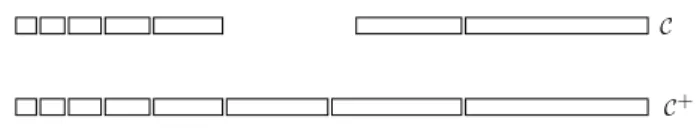
Definition 5.4 Let C = C1, C2, . . . , Cp−1, Cp, . . . , Cn be a list of clients. It is said that C is increased if the
new list of clients, denoted by C+, contains a new client Y with capacity w placed between clients C
p−1 and
Cp, i.e., wp−1 ≤ w ≤ wp. And, Cpincreases its capacity maintaining the position. If Cp′ denotes the actualized
client Cp and w′p its new capacity, then wp≤ w′p≤ wp+1. Hence, the transformed list of clients will be:
C+
= C1, C2, . . . , Cp−1, Y, Cp′, . . . , Cn, with wp≤ wp′ ≤ wp+1.
C+ C
Figure 1: Example of an increased list of clients
Definition 5.5 Let C = C1, C2, . . . , Cp−1, Cp, . . . , Cn be a list of clients. It is said that C is decreased if
the new list of clients, denoted by C−, contains one client less, let’s say client C
p. And, Cp+1 decreases
its capacity maintaining the position. If C′
p+1 denotes the actualized Cp+1 and w′p+1 its new capacity, then
wp≤ wp+1′ ≤ wp+1. Hence, the transformed list of clients will be:
C−
= C1, C2, . . . , Cp−1, Cp+1′ , . . . , Cn with wp≤ w′p+1≤ wp+1.
C− C
Figure 2: Example of a decreased list of clients
Note that this two definitions represents when a client arrives or leaves the system, but also includes a more general situation which is produced with the recursion of the assignation for one server after other. Figures 1 and a 2 shows how an increased and decreased list looks like. The following lemmas shows that increase or decrease the list of clients does not produce great changes at the moment of recompute the allocations. Lemma 5.6 Given C and S, a list of clients and one server. And, obtaining S(C) and CS (the clients
connected with S and the actualized list of clients, respectively) using Definition 5.1. If C is increased (or decreased) to C+ (or C−
) and Definition 5.1 is used to establish connections from C+ (C−
) with S. Then, there will be at most one new connection, one disconnection, and two changes in already existing connections for server S. And, the new actualized list of clients C+
S (C −
S) will be equal to (CS)+ ((CS)−), the previous
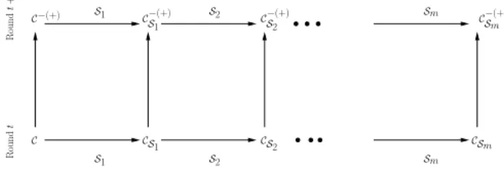
Lemma 5.6 is the brick to prove our main result, it is used as the base of an induction. Algorithm OSeq computes first server by server the allocations and then it goes round by round recomputing the allocations, where in each round it recomputes server by server again. The transformation of the list of clients (increased or decreased) represents the rounds, and Lemma 5.6 ensures that if the list of clients suffers a transformation, then for the first server there is at most one disconnection, one new connection, and two changes on the already existing connections. But also, it says that the actualized list of clients is a transformed list. Hence, applying again the Lemma for the second server, also it is possible to ensure that it has at most one disconnection, one new connection, and two changes on the already existing connections, and that the actualized list is a transformed list. Finally, applying recursively Lemma 5.6 for all the servers from S1 until Sm as it is showed in Figure 3 we can state our main result.
Theorem 5.7 When the online algorithm OSeq is used to solve the online version of MTBD, at most one new connection, one disconnection and two changes on already existing connections are produced per server per round. R ou n d t R ou n d t + 1 Sm Sm S2 S2 S1 S1 C−(+) C−(+) S1 C −(+) S2 C −(+) Sm CSm CS2 CS1 C
Figure 3: Application of Lemma 5.6 recursively first to server S1until Sm.
References
[1] D.P. Anderson. BOINC: A System for Public-Resource Computing and Storage. In 5th IEEE/ACM International Workshop on Grid Computing, pages 365–372, 2004.
[2] D.P. Anderson, J. Cobb, E. Korpela, M. Lebofsky, and D. Werthimer. SETI@ home: an experiment in public-resource computing. Communications of the ACM, 45(11):56–61, 2002.
[3] C. Banino, O. Beaumont, L. Carter, J. Ferrante, A. Legrand, and Y. Robert. Scheduling Strategies for Master-Slave Tasking on Heterogeneous Processor Platforms. IEEE Transactions on Parallel and Distributed Systems, pages 319–330, 2004.
[4] O. Beaumont, L. Eyraud-Dubois, H. Rejeb, and C. Thraves. Allocation of Clients to Multiple Servers on Large Scale Heterogeneous Platforms. INRIA Research Report, pages RR–6766, 2008.
[5] O. Beaumont, A. Legrand, L. Marchal, and Y. Robert. Pipelining Broadcasts on Heterogeneous Plat-forms. IEEE Transactions on Parallel and Distributed Systems, pages 300–313, 2005.
[6] D. Bertsimas and D. Gamarnik. Asymptotically optimal algorithm for job shop scheduling and packet routing. Journal of Algorithms, 33(2):296–318, 1999.
[7] Martin A. Brown. Traffic Control HOWTO. Chapter 6. Classless Queuing Disciplines. http://tldp.org/HOWTO/Traffic-Control-HOWTO/classless-qdiscs.html, 2006.
[8] Chandra Chekuri, Ashish Goel, Sanjeev Khanna, and Amit Kumar. Multi-processor scheduling to minimize flow time with ǫ resource augmentation. In STOC ’04: Proceedings of the thirty-sixth annual ACM symposium on Theory of computing, pages 363–372, New York, NY, USA, 2004. ACM.
[9] F. Chung, R. Graham, J. Mao, and G. Varghese. Parallelism versus Memory Allocation in Pipelined Router Forwarding Engines. Theory of Computing Systems, 39(6):829–849, 2006.
[10] L. Epstein and R. van Stee. Approximation Schemes for Packing Splittable Items with Cardinality Constraints. Lecture Notes in Computer Science, 4927:232, 2008.
[11] Leah Epstein and Rob van Stee. Improved results for a memory allocation problem. In Frank K. H. A. Dehne, J¨org-R¨udiger Sack, and Norbert Zeh, editors, WADS, volume 4619 of Lecture Notes in Computer Science, pages 362–373. Springer, 2007.
[12] L. Eyraud-Dubois, A. Legrand, M. Quinson, and F. Vivien. A First Step Towards Automatically Building Network Representations. Lecture Notes in Computer Science, 4641:160, 2007.
[13] Shelby Funk, Joel Goossens, and Sanjoy Baruah. On-line scheduling on uniform multiprocessors. Real-Time Systems Symposium, IEEE International, 0:183, 2001.
[14] B. Hong and V.K. Prasanna. Distributed adaptive task allocation in heterogeneous computing envi-ronments to maximize throughput. International Parallel and Distributed Processing Symposium, 2004. Proceedings. 18th International, 2004.
[15] B. Hubert et al. Linux Advanced Routing & Traffic Control. Chapter 9. Queueing Disciplines for Bandwidth Management. http://lartc.org/lartc.pdf, 2002.
[16] Bala Kalyanasundaram and Kirk Pruhs. Speed is as powerful as clairvoyance. J. ACM, 47(4):617–643, 2000.
[17] S.M. Larson, C.D. Snow, M. Shirts, and V.S. Pande. Folding@ Home and Genome@ Home: Using dis-tributed computing to tackle previously intractable problems in computational biology. Computational Genomics, 2002.
[18] CA Phillips. Optimal Time-Critical Scheduling via Resource Augmentation. Algorithmica, 32(2):163– 200, 2008.
[19] T. Saif and M. Parashar. Understanding the Behavior and Performance of Non-blocking Communica-tions in MPI. Lecture Notes in Computer Science, pages 173–182, 2004.
[20] H. Shachnai and T. Tamir. Multiprocessor Scheduling with Machine Allotment and Parallelism Con-straints. Algorithmica, 32(4):651–678, 2002.
[21] Hadas Shachnai, Tami Tamir, and Omer Yehezkely. Approximation schemes for packing with item fragmentation. Theory Comput. Syst., 43(1):81–98, 2008.
[22] G. Shao, F. Berman, and R. Wolski. Using effective network views to promote distributed applica-tion performance. In Internaapplica-tional Conference on Parallel and Distributed Processing Techniques and Applications. CSREA Press, June 1999.
[23] A. Siemion, J. Von Korff, P. McMahon, E. Korpela, D. Werthimer, D. Anderson, G. Bowera, J. Cobbb, G. Fostera, M. Lebofskyb, J. van Leeuwena, W. Mallardd, and M. Wagnerd. New SETI Sky Surveys for Radio Pulses. arXiv:0811.3046v1 [astro-ph], 2008.
Appendix
6
Proof of Lemma 5.2
Proof: In order to prove the lemma, it is necessary prove that the part of split client, which was not allocated in the server, is reinserted in the list between Cl−1and Cl+d+1, the border clients not allocated in the server.
On one hand, since the remaining part of the split client is smaller than the hole client, then we have: wl+d′′ < wl+d≤ wl+d+1.
On the other hand, due to C(l + 1) ≥ b, w′
l+d= b − C(l, l + d − 1), and w ′ l+d+ w ′′ l+d = wl+d we have: w′′ l+d = C(l, l + d − 1) + wl+d− b w′′l+d = wl+ C(l + 1) − b w′′ l+d ≥ wl ≥ wl−1
7
Proof of Lemma 5.6
Proof:Increased list Let Y be the new client, and w its capacity. Also, let C′ p and w
′
pdenotes the actualized Cp
and its new capacity, respectively. Due to the fact that C+ has a new client placed between C
p−1 and Cp, it
is possible to say that all the clients before Y maintains its position in the list, and all the clients after Y has an index shifted in one to a bigger index. Then, when C+(l, l + d − 1) is computed we have:
C+
(l, l + d − 1) = C(l, l + d − 1) for l + d − 1 < p C+(l, l + d − 1) = C(l − 1, l + d − 2) for p + 1 < l,
i.e., if the transformation does not affect the clients connected with S, the same clients will be connected after the list is increased. Consequently, no new connection is performed and the actualized list will be C+
S = (CS)+.
In the following, it is assumed that the transformation suffered by the list is among the clients connected with S. The proof is split for the three different cases in Definition 5.1.
The clients connected with server S satisfy condition (7): Let S(C) = Cl, Cl+1, . . . , Cl+d−1, C′l+d be
the clients connected with S. And, let CS = C1, C2, . . . , Cl−1, Cl+d′′ , Cl+d+1, . . . , Cn be the actualized list of
clients after the connection is done. (Both of them, S(C) and CS, defined before the list is increased.) Due
to the fact that w ≤ wpand wp′ ≤ wl+d−13, we have:
C+
(l, l + d − 1) = C(l, l + d − 1) + w + w′
p− wp− wl+d−1< b.
And, due to w ≥ wl+14 and wp′ ≥ wp, it is possible to say:
C+
(l + 2, l + d + 1) = C(l + 1, l + d) + w + w′
p− wp− wl+1≥ b. 3In the case p = l + d, Y appears between C
l+d−1and Cl+d. Then, C+(l, l + d − 1) = C(l, l + d − 1) because there are no new
client between Cland Cl+d−1. 4
In the case p = l + 1, Y appears between Cland Cl+1. Then, C+(l + 2, l + d + 1) = C(l + 1, l + d) because there are no new
Hence, either the new clients connected with S are S(C+
) = Cl, . . . , Y, Cp′, . . . , C ′
l+d−1and the actualized list
is equal to
CS+= C1, . . . , Cl−1, C ′′
l+d−1, Cl+d, Cl+d+1. . . , Cn.
Or, the new clients connected with S are S(C+) = C
l+1, . . . , Y, Cp′, . . . , C ′′′
l+d and the actualized list is
C+S = C1, . . . , Cl−1, Cl, C ′′′′
l+d, Cl+d+1, . . . , Cn.
In both cases, Y is the only new connection for S. And also, there is only one new client appearing in the new actualized list of clients, either C′′
l+d−1 or Cl. Finally, client Cl+d is actualized with a new
capacity. To conclude that C+
S = (CS)+, it is necessary to prove that: either w′′l+d ≤ wl+d ≤ wl+d+1 or
w′′ l+d ≤ w
′′′′
l+d ≤ wl+d+1 depending on what was the new connection and the new actualized list of clients.
The first case comes from the definition of C′
l+d and the initial assumption that wl+d ≤ wl+d+1. In the
second case, by definition we have w′′
l+d= C(l, l + d) − b and w ′′′′ l+d= C + (l + 1, l + d + 1) − b. And also: C+ (l + 1, l + d + 1) = C(l, l + d) + w + wp′ − wp− wl,
using the fact that wp≤ wp′ and w ≤ wl, it is possible to conclude C(l, l + d) ≤ C+(l + 1, l + d + 1) and then
w′′ l+d≤ w ′′′′ l+d. Hence, C + S = (CS)+.
The clients connected with server S satisfy condition (8): Let S(C) = C1, C2, . . . , Cl, Cl+1′ be the
list of clients connected with server S and CS = Cl+1′′ , Cl+2, . . . , Cn be the actualized list of clients after the
connection is done, (before the list is increased). Due to the transformation suffered by C, it is possible to say that: C+ (1, l) = C(1, l) + w + w′ p− wp− wl< b and C+ (1, l + 2) = C(1, l + 1) + w + wp′ − wp≥ b,
the first inequality is due to w ≤ wp and wp′ ≤ wl5. And the second inequality is due to w ≥ 0 and wp′ ≥ wp.
Hence, either S(C+) = C
1, . . . , Y, Cp′, . . . , Cl′ and the actualized list is
C+S = C ′′ l, Cl+1, . . . , Cn, or S(C+) = C 1, . . . , Y, Cp′, . . . , C ′′′
l+1 and the actualized list is equal to
C+ S = C
′′′′
l+1, Cl+1, . . . , Cn.
In both cases, Y is the only new connection for S. Also in the first case, it is possible to say that C′′ l is the
new client appearing in the new actualized list, and Cl+1 is a bigger fraction of Cl+1′ . In the second case, it
is possible to assume that there exist a new client Y but with capacity w = 0. And finally, by definition we have that w′′ l+1= C(1, l + 1) − b and w ′′′′ l+1= C + (1, l + 2) − b. Since, C+ (1, l + 2) = C(1, l + 1) + w it is possible to say that C+ (1, l + 2) ≥ C(1, l + 1) and then w′′′′ l+1≥ w ′′
l+1, to finally conclude that C +
S = (CS)+.
The clients connected with server S satisfy condition (9): Let S(C) = Cn−d+1, Cn−d+2, . . . , Cn be
the clients connected with S and CS = C1, C2, . . . , Cn−dbe the actualized list of clients after the connections
are performed. (Both of them, S(C) and CS, defined before the transformation is done.) In this case, due to
w ≤ wp and wp′ ≤ wn6 it is possible to say that:
C+
(n − d, n − 1) = C(n − d + 1, n) − wn+ w − wp+ w′p< b. 5
When w′
p> wland the transformation is among the first allocated clients, means that p = l + 1. Hence, Y is the l th client
and C+
(1, l) = C(1, l) + w − wl, what is smaller than b due to w ≤ wl. 6When w
Hence, if C+
(n − d + 1, n) ≥ b condition (7) is used to allocate clients into S. Therefore, S(C+
) = Cn−d+1, Cn−d+2, . . . , Y, Cp′, . . . , C
′
n, where Y is the only new client connected for S. And, the actualized list
of clients is (CS)+= C1, C2, . . . , Cn−d, C′′n. Here, C ′′
n is the new client appearing in the list, and since it is the
last client, then it is not necessary to prove nothing about the client after it. Otherwise, C+
(n − d + 1, n) < b and then the allocated clients into S are S(C+) = C
n−d+2, Cn−d+3, . . . , Y, Cp′, . . . , Cn with Y as the only new
connection for S. And, the actualized list CS+will be equal to CS = C1, C2, . . . , Cn−d, Cn−d+1.
Decreased list The proof for a decreased list is similar to the previous proof. Again, if the transformation of the list does not tach the clients connected with the server, then they will be connected again with the server and the actualized list will be the previous actualized list but decreased. Hence, it is assumed that the transformation affects the clients connected with the server. Also, the proof is split in the cases of Definition 5.1.
The clients connected with server S satisfy condition (7): Let S(C) = Cl, Cl+1, . . . , Cl+d−1, C′l+d be
the clients connected with S. And, let CS = C1, C2, . . . , Cl−1, Cl+d′′ , Cl+d+1, . . . , Cn be the actualized list of
clients after the connection is done (before the list is decreased). The decreased list is equal to C−
= C1, . . . , Cp−1, Cp+1, . . . , Cn, with wp ≤ w′p+1 ≤ wp+1. Then, we can
say that C−
(l − 1, l + d − 2) = C(l, l + d − 1) − wp+ wl−1− wp+1+ w′p+1 < b, because wl−1 ≤ wp and
w′
p+1≤ wp+1. Also we can say, C−(l + 1, l + d) = C(l + 1, l + d) − wp+ wp+1′ − wp+1+ wl+d+1≥ b, because
wp+1≤ wl+d+1 and wp≤ w′p+1. Therefore, it happens either:
S(C−) = Cl−1, Cl−2, . . . , Cp−1, C ′ p+1, . . . , Cl+d−1, C ′′′′ l+d and C − S = C1, . . . , Cl−2, C ′′′ l+d, . . . , Cn, or S(C− ) = Cl, Cl+1, . . . , Cp−1, C ′ p+1, . . . , Cl+d, C ′ l+d+1 and C − S = C1, . . . , Cl−1, C ′ l+d+1, . . . , Cn.
In both cases there is only one new connection for server S, either Cl−1 or Cl+d+1. For the side of the
actualized list, in both cases there is one client less, either Cl−1 or Cl+d. And, since C−(l − 1, l + d − 2) <
C(l, l + d − 1) then w′′′ l+d≤ w
′
l+d. Also, wl+d+1≤ wl+d+1. And then, CS− = (CS)−.
The clients connected with server S satisfy condition (8): Let S(C) = C1, C2, . . . , Cl, Cl+1′ be the
list of clients connected with server S and CS = Cl+1′′ , Cl+2, . . . , Cn be the actualized list of clients after the
connection is done (before the list is decreased). The decreased list of clients C−
= C1, C2, . . . , Cp−1, Cp+1′ , . . . , Cn is affecting the already clients connected
with S. Then p ≤ l + 1. Therefore, using wp ≤ wp+1′ ≤ wp+1 we have either C−(1, l − 1) = C(1, l) − wp−
wp+1+ w′p+1< b and C −
(1, l + 1) = C(1, l + 1) − wp+ w′p+1− wp+1+ wl+2≥ b. Hence, the list of connected
clients to server S and the actualized list of clients are either S(C−) = C1, C2, . . . , Cp−1, C ′ p+1, . . . , Cl, C ′′′′ l+1 and C − S = C ′′′ l+1, Cl+2, . . . , Cn, or S(C− ) = C1, C2, . . . , Cp−1, C′p+1, . . . , Cl+1, Cl+2′ and C − S = C ′′ l+2, Cl+3, . . . , Cn.
In the first case, there is no new connection for server S. And, since C−(1, l − 1) < C(1, l), then the size of the
first element of the actualized list of clients (C′′′′
l+1) is smaller than the size of the first element of the previous
actualized list of clients (C′′
l+1), therefore C −
S = (CS)−. In the second case, there is one new connection to
server S, Cl+2. And, the actualized list of clients C −
S is the previous actualized list of clients decreased (CS)−.
The clients connected with server S satisfy condition (9): Let S(C) = Cn−d+1, Cn−d+2, . . . , Cn be
the clients connected with S and CS = C1, C2, . . . , Cn−dbe the actualized list of clients after the connections
are performed (before the transformation is done). The new list C−
is equal to C1, C2, . . . , Cp−1, Cp+1′ , . . . , Cn. And, either p = n − d or p ≤ n − d + 1
(if it is smaller than n − d, then it does not affect the clients connected with the server). Hence, either C−(n−d+1, n) = C(n−d+1, n)−w
p+1+w′p+1or C
−(n−d+1, n) = C(n−d+1, n)−w
p+1+wp+1′ −wp+wp−1. In
both cases C−(n−d+1, n) < b, due to w
p+1≥ w′p+1and wp≥ wp−1. Therefor, S(C−) = Cn−d, Cn−d+2′ , . . . , Cn
or S(C−) = C
n−d, Cn−d+2, . . . , Cp+1′ , . . . , Cn, with Cn−d as the only new connected client to S. Finally, in
both cases C−
S = C1, C2, . . . , Cn−d−1 = (CS)−.
8
Proof of Theorem 5.7
Proof: The proof is by induction over the order of the list of servers. The first step of the induction is the first sever. It is analyzed whether the first server has a new connection in a round and then how this affects the new connections of the rest of the servers. Lemma 5.6 is the basis of the analysis. First, note that from one round to another the list of clients is increased, decreased or it stays equal. If the list of clients stay equal then the algorithm has nothing to do, and no new connections are established. When the list of clients has increased or decreased, to apply Lemma 5.6, according to the case for the first server, let us continue applying the same lemma to establish the connections for all servers, concluding that all of them will have at most one new connection and that the list will be ready for the next server. This argument is valid for any round, and hence the result is concluded.