Publisher’s version / Version de l'éditeur:
Vous avez des questions? Nous pouvons vous aider. Pour communiquer directement avec un auteur, consultez la première page de la revue dans laquelle son article a été publié afin de trouver ses coordonnées. Si vous n’arrivez pas à les repérer, communiquez avec nous à [email protected].
Questions? Contact the NRC Publications Archive team at
[email protected]. If you wish to email the authors directly, please see the first page of the publication for their contact information.
https://publications-cnrc.canada.ca/fra/droits
L’accès à ce site Web et l’utilisation de son contenu sont assujettis aux conditions présentées dans le site
LISEZ CES CONDITIONS ATTENTIVEMENT AVANT D’UTILISER CE SITE WEB.
American Control Conference (ACC) 2003 [Proceedings], 2003
READ THESE TERMS AND CONDITIONS CAREFULLY BEFORE USING THIS WEBSITE.
https://nrc-publications.canada.ca/eng/copyright
NRC Publications Archive Record / Notice des Archives des publications du CNRC :
https://nrc-publications.canada.ca/eng/view/object/?id=c59b1c49-03e9-4410-acb0-8754aa6e55e3
https://publications-cnrc.canada.ca/fra/voir/objet/?id=c59b1c49-03e9-4410-acb0-8754aa6e55e3
NRC Publications Archive
Archives des publications du CNRC
This publication could be one of several versions: author’s original, accepted manuscript or the publisher’s version. / La version de cette publication peut être l’une des suivantes : la version prépublication de l’auteur, la version acceptée du manuscrit ou la version de l’éditeur.
Access and use of this website and the material on it are subject to the Terms and Conditions set forth at
Modeling an Auto-Synchronizing Laser Range Scanner
MacKinnon, David; Blais, François; Aitken, D.
National Research Council Canada Institute for Information Technology Conseil national de recherches Canada Institut de technologie de l'information
Modeling an Auto-Synchronizing Laser Range
Scanner*
MacKinnon, D., Blais, F., and Aitken, D.
June 2003
* published in American Control Conference (ACC 2003). June 4-6, 2003.
Denver, Colorado, USA, TP09-04, pp. 1-6. NRC 45840.
Copyright 2003 by
National Research Council of Canada
Permission is granted to quote short excerpts and to reproduce figures and tables from this report, provided that the source of such material is fully acknowledged.
Modeling an Auto-synchronizing Laser Range Scanner
David K. MacKinnon1
[email protected] Francois Blais 2
[email protected] Victor C. Aitken 1 [email protected] 1 Department of Systems and Computer Engineering, Carleton University, Ottawa, Ontario, Canada, K1S 5B6
2 Institute for Information Technology, National Research Council of Canada, Ottawa, Ontario, Canada, K1A 0R6
Abstract
This paper presents a Matlab model of an auto-synchronizing variable-resolution laser scanner. The model simulates the optical path of the laser through the scanner to the target surface and the image path from the target surface to the CCD array. The environment and the position of the scanner at any point in time in the environment are also modeled. Results obtained after calibrating the system to an actual laser scanner prototype closely match the data collected using that scanner.
1 Introduction
The National Research Council of Canada (NRC) developed a laser range scanner (LRS) to perform object detection and tracking at ranges between 0.5-metres and 2-kilometres [1]. The system can obtain range and intensity information using either a raster scan pattern or a Lissajous scan pattern. When in imaging mode the scanner uses a raster scan pattern to obtain dense range or intensity maps of the scene or object. In real-time tracking mode the system uses one or more Lissajous scanning patterns to obtain sparse range or intensity maps [4].
Figure 1: LRS unit
Development work using the LRS has been limited due to the small number of LRS units available and the expense of building each unit. The ability to test algorithms for motion distortion is limited to availability and cases in which the LRS unit is not at risk of being damaged. The LRS has been integrated with the Space Vision System (SVS) that is being developed by Neptec Design Group (NDG) for the Canadian Space Agency (CSA) but testing under space conditions, such as in Figure 2, is difficult to perform on earth [7]. An accurate model of the scanner in a customizable environment would allow NRC and NDG to evaluate scanner performance without the cost of transportation and testing in space.
Figure 2: LRS on Space Shuttle mission STS-105 (photo courtesy of NASA)
In the current study we are interested in performing a comprehensive evaluation of the robustness of various edge detection algorithms applied to sparse range data. This development work would require extensive use of an existing LRS unit so it was decided to develop an accurate model so that much of this work could be performed off-line.
Figure 3: Internal representation of a typical LRS unit (Reprinted from Figure 1 of [7])
2 Model development
A model was developed using optical ray propagation to determine the point of intersection of a laser beam with an object surface in the environment. An inverting camera pinhole model was used to correlate the intersection point in the camera frame of reference to the position on the CCD array.
The first stage in the development of a useful model was the examination of the optical path through the auto-synchronized triangulation system. Figure 3 shows a representation of a LRS unit. Model development was restricted to the simulation of short (0.5 to 2 metres) and medium (2 to 10 metres) range data collection. The simulation was further simplified by only considering the principal optical path. Range data was found as the position of the theoretical signal peak on a simulated linear CCD array. The development of the model used in this study was based on the calibration model used by Beraldin et al [1] [3] [5], and Blais et al [2] [6].
Figure 4: Internal arrangement of the CCD array (left) and mirrors (right)
The model was developed using Matlab and the simulation environment consisted of a series of modular scripts. The modular structure provided a logical framework to verify each component. The system was designed such that it could be tailored to a range of test conditions and could be calibrated to any LRS unit. The simulation environment consisted of three components, the output LRS model (OLM), the environmental interaction model (EIM), and the input LRS model (ILM).
2.1 Output LRS Model
The OLM generated a ray corresponding to the laser output along the z-axis of the LRS frame of reference. The orientation of the ray depended upon the deflection angles of the x-axis and y-axis mirrors as seen in Figure 3. The mirror angles were controlled by entering a value between –1 and 1 corresponding to the normalized minimum and maximum mirror angles. According to [3] the prototype of Figure 4 of the LRS has a maximum field of view (FOV) of 30º by 30º. The prototype of Figure 2 has a larger FOV. Here we defined the maximum and minimum angular deviations as 15º and -15º respectively. The galvanometers controlling each mirror are driven by 16-bit D/A converters [3] so the –1 to 1 value was quantized [8] and converted to an integer value between –32768 and 32767.
2.2 Input LRS Model
The ILM was provided the location in the LRS frame of reference of the intersection of the output ray with a surface in the environment. This information was used to determine the image path to the intersection point with a plane representing the surface of a linear CCD array. The distance to this intersection point was used to calculate the expected location of the signal peak. The peak location was normalized to a value between 0 and 1. The CCD array and its peak detector produce a 16-bit value corresponding to 1/64 of a pixel [3] so the peak value was quantized [8] and converted to an integer between 0 and 32767. If the intersection point and the output ray origin are the same point then a peak value of 0 is returned to indicate no peak location.
2.3 Environmental Interaction Model
The environmental model consisted of the position and orientation of the LRS in the environment and planar surfaces representing objects in the environment. The path of the ray generated by the OLM was translated into the environmental frame of reference using the YPRT (Yaw, Pitch, Roll, Translate) convention. The shortest path to intersection of all possible planar surfaces was determined and used to calculate the point of intersection of the ray with a surface in the environment. If no surface was intersected then the intersection point was defined to be the origin of the ray. This provided a way to alert the ILM that no return signal would be detected. The model currently does not consider shadow effects nor does it simulate the intensity of the return signal.
Figure 5: Graphical representation of the LRS position (black dot) laser path (solid line) and an object composed of planar surfaces. All units are in metres.
3 Model calibration
The LRS model can be calibrated to simulate the results of any LRS unit. In this study we calibrated the model to match the results that would be generated using the LRS unit called Space 40 [4]. The calibration process involved matching the results generated by the galvanometers and the peak detector.
3.1 Galvanometer Calibration
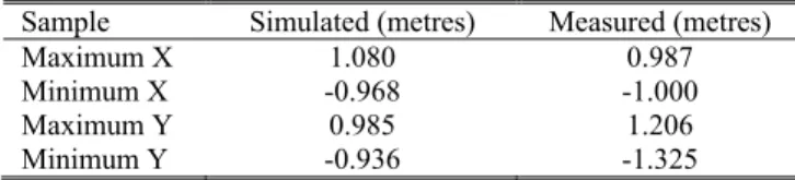
A 256-point Lissajous scan was obtained at each of the galvanometer extents for each galvanometer. The maximum and minimum galvanometer values were obtained and used to map the LRS model galvanometer results to the observed galvanometer results obtained with the prototype of Figure 1. The direction of the mapping was confirmed by obtaining the corresponding x and y Cartesian coordinates of the points corresponding to the maximum and minimum galvanometer values. The galvanometers were considered to be linear devices so no further fitting was performed. Table 1 shows typical measured and simulated results
Table 1: Comparison of Measured and Simulated X and Y Cartesian values.
Sample Simulated (metres) Measured (metres) Maximum X Minimum X Maximum Y Minimum Y 1.080 -0.968 0.985 -0.936 0.987 -1.000 1.206 -1.325 3.2 Peak Calibration
Peak values were obtained using the system of Figure 1 at distances between 1-metre and 9-metres. Linear regression was used to obtain a best-fit line to predict the observed peak values based on model-generated peak and galvanometer values. Simulated peak values and x-galvanometer values were found to significantly predict the observed peak values.
Figure 6 shows the error associated with the corrected peak values. Even though all the optical aberrations of the system are not completely simulated, the observed peak errors are small enough to provide useful results. The current fit has a standard error of the estimate of 16.7, or ¼ of a pixel of the CCD, so is accurate to within an acceptable error margin. Note that a peak location noise of 1/8 of a pixel is typical of such a system. The fit has coefficient of determination (R2) of almost 1 indicating an acceptable linear fit assuming the data is almost linear.
Figure 6: Expected minus Observed peak values after correction for samples between 1-metre to 10-metres.
3.3 UV to Cartesian conversion
The UV coordinates system used throughout this study is a variation of the spherical coordinate system. U corresponds to the deflection along the (y-z) plane and V corresponds to the a deflection along the (x,z)-plane. The axis of the U deflection is almost the same as the origin of the camera frame of reference. However, the V deflection axis is offset from the origin by an amount hx corresponding to the separation between the x-axis and
y-axis mirrors. Blais et al examined the relationship between the
Cartesian coordinate system and the UV coordinate system [6]. Another way to convert UV to Cartesian coordinates involves a more comprehensive knowledge of the LRS intrinsic parameters. These intrinsic parameters are the CCD length LCCD, the fixed
mirror angles βout and βin, the movable mirror angles at zero
deflection βx and βy, the separations between the fixed and
movable mirror centres and the LRS origin hx, hy and hz, and the
focal length f.
Figure 7: Simplified and unwrapped 2D representation of the 3D optical path through the system as seen in Figure 3 Υ represents the target and Λ the collecting lens.
Figure 7 shows the unwrapped path from a point of intersection Υ with a target in the environment through the collecting lens axis Λ to a point on the CCD array. The arrangement forms two similar triangles. The triangle on the lower left can be characterized as having height Ph, and base length Pb. If we let p denote the
location of the detected peak on the CCD array then we can find
sin( ) h P = f + p βCCD and (1) cos( ) b P = p βCCD . (2)
If we assume that the imaging axis and the laser path are parallel then we can calculate the separation between the projected lens origin Λ and the projected laser origin Γ using
cos( ) sin( ) 2 sin( ) cos( ) sin( ) sin( ) hx out U D hx U out hx in U hx U in β β β β = + − − + (3)
where βout is the angle of the fixed output mirror, βin is the angle of
the fixed input mirror and U is an estimator for the deflection of the laser (line starting at Γ and passing through the point of reflection with the y-axis mirror f3) and the imaging axis (line
starting at Λ and passing through the point of reflection with the y-axis mirror a3) along the (x,z) plane. The offsets hx, hy and hz are
visible in Figure3. It can be shown that the deflection of the laser axis is
2 2
U out =π − βout − βx +2θ
2
(4) Similar triangles are used to relate the projection on the CCD to the position of the point in space. The distance Z from Γ to Y is found using
where βx is the zero-angle deflection of the x-axis mirror and θ is
the additional deflection of the x-axis mirror due to the
galvanometer. The deflection of the optical axis is Z Dcos
( )
U Ph Dsin(U )i Pb
= − i . (12)
2 2
Uin = βin − βx + θ . (5) Two corrections are required to include the unwrapped length of the projection from a3 to the collecting lens axis Λ. These are
defined by The system is generally designed such that Uout≈ Uin.. This is
accomplished by making βin, βout and βx, as close to π/4 as
possible. Future equations can therefore be simplified by defining an estimator U ≈ Uin ≈ Uout where U = 2θ.
cos( ) sin( ) sin( ) hx out U dx hx U out β β = − + and (13)
The intersection point f3 of the laser with the y-axis mirror in the
LRS frame of reference can now be estimated. It can be seen in Figure 3 that the intersection of the laser with the y-axis mirror is in the (x,y)-plane so we define f3z as zero. We then calculate
sin( ) sin( ) sin( ) hx out U d y U out β β = + . (14) tan( ) 3
f y = hy −hz φ +βy (6) The corrected distance can now be calculated using
where β ≈ π/4 and cos( ) sin( ) tan( ) 3 sin( ) 3 hx out U f x hx y U out β β = + + − f U
. (7) − + 2 2 2 2 ( 3 tan( )) ( 3 ) Zc Z Dl dx dy f y U dy f y = − − + + (15)where Dl is the distance from the lens to the x-axis mirror. A
further correction is needed to translate Z into a distance R from the LRS origin to the point of intersection Y. The projection of Zc
is first calculated using The angle Ui between the z-axis and the imaging axis is estimated
by first calculating the coordinates of a theoretical point 1-metre from the camera. This is found by
tan( ) 3 tan( ) 3 1 Yx f x U Yy f y V Yz ′ + ′ = + ′
(8) tan ( )2 tan ( ) 12 Z c Zcz U V = + + . (16)This is used to calculate the Cartesian coordinates of the point Y using
where V=2Φ is an estimate for the deflection of the y-axis mirror resulting from a galvanometer deflection Φ. From Figure 7 it can be see that if Z and N are known then Ui can be found. The
coordinates of Y as the intersection of the laser with a surface in the environment are not known but an estimate of the distance to a point 1-metre from the LRS can be calculated. We define
tan( ) 3 tan( ) 3 f Z U Yx x cz Yy f y Zcz V Yz Zcz + = +
. (17) 2 2 ( 3 ) ( 3 ) 2Z′= f x −Yx′ + f y −Yy′ + ′ (9) Yz The distance from the origin to the point of intersection can then be calculated using
and the projection onto the z-axis 2
( 3 ) 2
N′= f y −Yy′ + ′ . (10) Yz
2 2 2
R = Yx +Yy +Yz . (18)
We can now find Ui using
( )
1
cos N sgn( )
U i = − Z′′ U . (11)
It can be seen in Figure 8 that the calculated range method provides a more accurate range measurement in the 1 to 10-metre range than calculating the range using calibration-based linear fitting. The calculated and actual range values are indistinguishable on the graph. The discrepancy between the calibration-based linear fit and calculated range values exists because the peak value is not linearly related to the range. In practice the linear fit method is used to quickly obtain range estimates within predefined range limits when speed is preferred
over precision. More precise methods are employed when precision is required.
Figure 10: Lissajous scan obtained using the LRS in Figure 1 Figure 8: Comparison of range estimation methods using
LRS Model simulator.
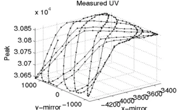
Figure 11: Lissajous scan obtained using the simulated LRS calibrated for the LRS in Figure 1
Figure 9: Lissajous scan of a simple box modeled in Figure 5
4 Results
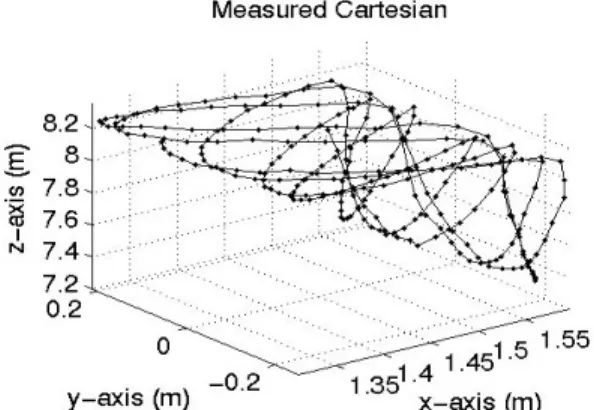
The position of a box, seen in Figure 9, with respect to the scanner of Figure 1 and their relative orientation were carefully measured and recorded. Three Lissajous scans of 256 data points each were performed with each scan repeated 10 times. The position of the box and orientation of the scanner were modeled using the Matlab simulation environment. Figure 10 shows a simple scan of the upper edge of the box in UV coordinates and Figure 13 shows the same scan in Cartesian coordinates. Figure 11 shows the results in UV coordinates obtained using the simulation and Figure 14 shows the same scan in Cartesian coordinates. Figure 12 compares the unwrapped Lissajous scans. It can be seen that the results obtained using the simulated system closely resemble the results obtained using the real scanner. The discrepancy between simulated and peak values is approximately 0.3 percent of the peak value in Figure 12. A discrepancy can be noted at each peak representing the difference between an ideal flat surface (convex peak) obtained using the simulation and a real surface curved slightly away the scanner.
Figure 12: Comparison of unwrapped measured (dotted line) and simulated (solid line) Lissajous scan peak values. Peak values are in the range 0 to 32767.
X- and Y-axes values are 16-bit integers corresponding to the angular deflection of the associated mirror. Peak values are 16-bit integers corresponding to the detected location of the peak on a linear CCD array
Figure 13: Lissajous scan from Figure 10 translated into Cartesian coordinates using calibration-based linear fit
Figure 14: Lissajous scan from Figure 11 translated into Cartesian coordinates based on LRS intrinsic parameters.
5 Conclusions
The LRS model environment appears to produce results that accurately represent real data that could be obtained from a corresponding LRS unit for range values between 1-metre and 9-metres. The LRS model can be configured for any LRS unit so results obtained from development work using the LRS model can be validated using the corresponding LRS unit. Simple objects in the environment can be simulated and the results obtained from an interaction between the LRS model and the simulated environment closely approximate results obtained from similar real-world interactions. The LRS model can be used to accurately examine scanner performance under adverse conditions without posing a risk to an actual LRS unit. The LRS model uses Matlab scripts so it is easily ported to other systems running Matlab of a similar or higher version. Development work can now be performed using the LRS model without the researcher requiring continuous access to an LRS unit.
Acknowledgments
D. MacKinnon thanks the Natural Science and Engineering Research Council of Canada (NSERC) for providing financial
support for this research, and the National Research Council of Canada (NRC) for providing facilities and equipment. The authors would also like to thank Neptec Design Group for their support and assistance, and Materials and Manufacturing Ontario for providing additional project funding
References
[1] Beraldin, J.-A., Blais, F., Rioux, M., Cournoyer, L., Laurin, D., and MacLean, S.G. "Eye-safe digital 3D sensing for space applications." Optical Engineering Vol.39, No.1, January (NRC 43585): Society of Optical Instrumentation Engineers, 2000. pp.196-211.
[2] Blais, F., Beraldin, J.-A., El-Hakim, S.F., and Cournoyer, L. "Real-time Geometrical Tracking and Pose Estimation using Laser Triangulation and Photogrammetry.'' Proceedings of
the Third International Conference on 3-D Digital Imaging and Modeling 28 May-1 June, Quebec, Quebec (NRC
44180): IEEE, 2001. pp 205-212.
[3] Beraldin, J.-A., El-Hakim, S.F., and Cournoyer, L. "Practical range camera calibration.'' SPIE Proceedings of Videometrics
II Vol.2067, Boston, MA, 7-10 September (NRC 35064):
SPIE, 1993. pp.21-31.
[4] Blais, F., Beraldin, J.-A., Cournoyer, L., El-Hakim, S.F., Picard M., Domey, J., Rioux, M., Christie, I., Serafini, R., Pepper G., MacLean S.G., and Laurin D. . "Target Tracking Object Pose Estimation, and Effect of the Sun on the NRC 3-D Laser Tracker." Proceedings of iSAIRAS-2001 Montreal, Quebec, June (NRC 44876): 2001.
[5] Beraldin, J.-A., Blais, F., Rioux, M., Cournoyer, L., Laurin,D., and MacLean, S. "Short and medium range 3D sensing for space applications." SPIE Proceedings of Visual
Information Processing VI (Aerosense '97) Vol.3074,
Orlando, FL, 21-25 April (NRC 40170): SPIE, 2000. pp.29-46.
[6] Blais, F., Beraldin, J.-A., and El-Hakim, S.F. "Range error analysis of an integrated time-of-flight, triangulation, and photogrammetry 3D laser scanning system." SPIE
Proceedings of AeroSense Vol.4035, Orlando, FL, 24-28
April (NRC 43649): SPIE, 2000.
[7] Blais, F., Couvillon, R.A., Rioux, M., and MacLean, S.G. "Real-time tracking of objects for space applications using a laser range scanner.'' Proceedings of the AAAI Conference on
Intelligent Robots in Field, Factory, Service and Space
Vol.II, Houston, TX, 20-24 March (NRC 37109): 1994. pp.464-472.
[8] Oppenheim, Alan V., and Schafer, Ronald W., Buck, John R. "Discrete-Time Signal Processing, 2nd edition.'' Upper Saddle River, New Jersey: Prentice-Hall, Inc., 1999, pp.190-193