The central city : why the comeback?

(1)

The Central City: Why the Comeback?

By Scott Nguyen

B.A., Economics, with Honors, 2003 University of California at Berkeley

Submitted to the Department of Architecture in partial fulfillment of the Requirements for the Degree of Master of Science in Real Estate Development

at the

Massachusetts Institute of Technology September, 2006

The author hereby grants to MIT permission to reproduce and to distribute publicly paper and electronic copies of this document in whole or in part in any medium now known or hereafter created. Signature of Author_______________________________________________________ Scott T. Nguyen Department of Architecture July 28th_{, 2006} Certified by______________________________________________________________ William C. Wheaton Professor of Economics Thesis Supervisor Accepted by_____________________________________________________________ David M. Geltner

Chairman, Interdepartmental Degree Program in Real Estate Development

(2)

The Central City: Why the Comeback? By

Scott Nguyen

Submitted to the Department of Architecture on July 28, 2006 in partial fulfillment of the requirements for the Degree of Master of

Science in Real Estate Development

Abstract

Recently, scholars and non-scholars alike have written and spoken much about the reversal of urban sprawl and the in-migration of young professionals and empty nesters. The objective of this study is first, to examine the relative city performance for the three defined metrics to determine whether cities are leading or lagging their MSAs in each respective metric and second, to determine how differences in relative performance correlate to the independent variables. Additional analyses will be performed to determine changes in household composition and relationships between supply growth and demand growth.

This paper, using OLS regression techniques, examines the correlation between various measures of relative city to MSA growth performance (specified as relative population, housing unit and property value growth) and various independent variables for a

representative sample of seventy three metropolitan areas. The study period includes data from 2000 to 2004. The twenty eight independent variables can be categorized into three major groups: (1) Demographic Characteristics (2) Environmental Characteristics and (3) Transportation Statistics.

The results show that, on average, central cities perform worse than their MSAs in terms of housing unit and population growth while outperforming in terms of property value growth. In central cities, housing units are growing faster than population, indicating either shrinking household size or increases in investor/second home demand. Considerable variation exists and averages do not tell the whole story. Certain independent variables, namely roadway miles and transit miles have strong correlations to relative growth metrics while others such as the city’s proportion of total MSA population have no observable relationship. Another surprising result is that a city’s proximity to a water amenity has negative correlation to its relative population, housing unit and property value growth rate.

Thesis Supervisor: William C. Wheaton Title: Professor of Economics

(3)

TABLE OF CONTENTS

Table of Contents... - 3 -

Acknowledgments... - 5 -

I. Introduction ... - 6 -

Section 1.1 Urban Exodus... - 6 -

II. Prior Research... - 11 -

III. Specific Area of Study and Hypothesis... - 19 -

Section 3.1 Introduction to Specific Area of Study... - 19 -

Section 3.2 Hypotheses... - 21 -

IV. Methodology... - 22 -

Section 4.1: Data Sources and Discussion of Variables... - 24 -

Section 4.1.1 Dependent Variables... - 24 -

Section 4.1.2 Independent Variables... 26

Section 4.1.3 Statistical Sample... 26

-V. Regression Results ... - 30 -

Section 5.1 City minus MSA Population Growth (2000-2004 Annualized) ... - 30 -

Section 5.1.1 Dependent Variable Transformation... - 31 -

Section 5.1.2 Regression Results and Discussion ... - 32 -

Section 5.2 City minus MSA Housing Unit Growth (2000-2004 Annualized) ... - 38 -

Section 5.3 Housing Unit Growth vs. Population Growth (2000-2004 City Only)... - 47 -

Section 5.4 Population minus Housing Unit Growth (City Only) ... - 50 -

Section 5.5 City Housing Unit Growth... - 56 -

Section 5.5.1 Dependent Variable ... - 56 -

Section 5.6 Housing Unit Growth vs. Property Value Growth (City minus MSA)... - 64 -

Section 5.6.1 Quadrant I Discussion... - 66 -

Section 5.6.2 Quadrant II Discussion ... - 67 -

Section 5.6.3 Quadrant III Discussion ... - 68 -

Section 5.6.4 Quadrant IV Discussion... - 68 -

Section 5.7 City minus MSA Housing Unit Growth by Quadrants ... - 70 -

Section 5.8 Property Value Growth (City minus MSA)... - 77 -

VI. Conclusion and Further Research... - 85 -

Bibliography ... - 90 -

(4)

Appendix II: City minus MSA Performance Metrics... - 94 -

Appendix III: City Performance Metrics... - 96 -

Appendix IV: Cities by Quadrant ... - 98 -

(5)

ACKNOWLEDGMENTS

I would like to thank my family and friends for their support and patience during this sometimes frustrating, but always intellectually stimulating thesis period. I hope the result is worth your suffering. Finally I would like to thank Professor Wheaton for providing me with guidance, data and thorough answers to my incessant questions.

(6)

I. INTRODUCTION

Today, urban planners, brokers and real estate developers confidently speak of the groundswell of population moving back into America’s core cities. Many claim that sprawl is reversing. At a 1998 Association of Collegiate Schools of Planning Conference, panelists stated that the housing and the population shift associated with it is one of the best ways to revitalize downtown (Sohmer and Lang, 1999). To them, this demographic shift has already begun and will only increase in magnitude as the baby boom generation enters their golden years.

Section 1.1 Urban Exodus

Scholars cite various reasons for the decline of downtown areas following World War II. Sohmer and Lang blame city planners for implementing the “policies of the 1960s and 1970s that over-zoned for office and retail uses and deliberately excluded residences from the central business district” (1999). Duany claims “somewhere along the way, through a series of small and well-intentioned steps, traditional towns became a crime in America” (Duany, Plater-Zyberk & Speck, 2000). He continues to explain the acceptance of sprawl by stating, “one of the largest segments of our economy, the homebuilding industry, developed a comprehensive system of land development practices based upon sprawl, practices that have become so ingrained as to be second nature” (Duany et al., 2000 ).

These policies mentioned by Sohmer and Lang “conspired to encourage urban dispersal” (Duany et al., 2000). The most significant of these, the loan programs

(7)

administered by the Federal Housing Administration and Veterans Administration, provided end-user funding for the purchase of eleven million new single-family suburban homes with interest rates that resulted in mortgage payments that typically cost less than rent. As a result, these programs discouraged the renovation of existing housing or even the construction of new housing of more downtown-amenable types such as row houses and mixed-use buildings. In combination with these policies, the Interstate Highway Act of 1956 provided ninety billion federal dollars to construct forty-one thousand miles of highway, other federal and local subsidies provided further incentive to build roads, and the general neglect of transit systems all conspired to make automotive commuting cheap and easy for everyone. Given the improved highway system and degrading transit system, most returning GIs migrated from the central city to the periphery. Soon after, the retail followed the residents but since the subdivisions were funded only for residential development, the new retail had to locate separate from the population (Duany et al., 2000). Jobs remained downtown for some time, with people living in the periphery and commuting downtown as in the classic mono-centric city model (Wheaton, 1995). However, the situation changed in the 1970s when corporations moved their offices closer to their CEOs, who by this point lived in the suburbs. As a result, the mono-centric city became poly-centric and living, shopping and working all moved out of the center city, leaving the core to decay.

While the population acted rationally and moved outwards due to the new economic framework imposed by government programs, they would then be bound by law to sprawl through single-use zoning. Single-use zoning, very useful in Europe’s industrialized cities to separate factories from residential areas, in America, expanded to

(8)

separate everything from everything else (Duany et al., 2000).1_{As a result, dependency on}

the car has developed and suburban areas were better suited for the parking needs of a car-dependent citizenry. The pattern has continued unabated for fifty years and today results in California growing by the size of a Massachusetts every decade.2

Clearly, an in-migration will have significant impacts on policy and business decisions. Sophisticated urban planning will become critical to prevent a repeat of failed urban planning and renewal experiments of the 1960s and 1970s. Real estate developers, as the ultimate satisfiers of demand for built space, must understand the nature and extent of this shift so that they can develop buildings that have the right product mix in the right location.

1_{The typical zoning code today has dozens of land use designations separating not only factories from residential but low} density from medium from high density residential. Offices and retail are often separated in the same manner.

2_{And this land growth is not equal with population growth: From 1970-1990 Los Angeles grew 45% in population and} 300% in land use.

(9)

Section 1.2 Theories on the Move Back Downtown

Various reasons have been given for the move back to the core city, many based on conjecture. According to Eugenie Birch of University of Pennsylvania, “anecdotal evidence suggests that people are living downtown because they want to be near work places and cultural amenities, and because they enjoy a bustling environment” (1998). The typical story told involves an empty nester couple who wish to sell their large, mostly empty suburban home for a smaller, more convenient urban condominium or townhouse. Adding to empty nester couples are mid to late twenties echo boomers, the children of the baby boomers, wishing to move downtown to remain close to work and to each other. Environmentalists cite rising fuel costs, loss of open space and increased air pollution as additional reasons that dense downtown living can be good for the pocketbook and your health (Sierra Club, 2006).

Drawing the diaspora back into central cities can provide significant and lasting benefits to the city. Average commutes, already at 24.3 minutes in 2003, can be significantly shortened by eliminating commuting or allowing city residents to reverse-commute to suburban offices (American Community Survey, 2003). The reduced vehicle dependence will result in better air quality and reduced rush-hour traffic jams. Mixing the uses by adding residential will create a safer, 24-hour city with retail establishments open after office hours. The vitality of pre-WWII central cities will return. Additionally, the growing central city population will draw businesses, office and retail back into the city, increasing tax base and removing the stigma associated with city living.

(10)

However, much of the talk about re-urbanization has been based on anecdotal evidence and conjecture. Specifically, the aging baby boomers are frequently cited as the source of this urban population growth (Baker, 2006). While the data exists, other than very recent studies, little rigorous analysis has been done to prove or disprove this theory. This thesis attempts to add to the body of knowledge concerning the nature, extent, and geographical distribution of this supposed move back to the core city by examining the relationship between central city growth and external factors such as Percent Sunshine per Year. Rather than only describing the demographic changes that have occurred in the past, I hope to lay a foundation for creating a model that can help predict where central city growth will occur in the future. A definitive, data-based answer will improve the decision-making ability of industry participants in regards to what, how and where to build the next generation of buildings.

In the following chapter, I will review the existing literature on the topic and draw out similarities and differences amongst the different points of view. Chapter 3 will then expand upon the questions I seek to answer and how they intertwine with existing research. I will also hypothesize on the results of my regression analysis. Chapter 4 will detail the analysis methodology and define the dependent and independent variables to be used. Results and analysis will follow in Chapter 5 with Chapter 6 will wrap up with conclusions and recommendations for further research.

(11)

II. PRIOR RESEARCH

A significant amount of research has been done by The Brookings Institution’s Center on Urban and Metropolitan Policy. Eugenie Birch, an urban planning professor at University of Pennsylvania, conducted a survey of 24 cities nationwide in 1998 study entitled

A Rise in Downtown Living which examined the 1998-2010 population growth expectations3

from city officials. The involved city officials did not make clear nor standardize their projection methodology, so this study cannot to be considered strictly rigorous. Regardless, this report initiates the recent discussion on re-urbanization. Based on the survey, city officials’ growth expectations ranged from 1.5% for Los Angeles to 303% for Houston.

Figure 1: Expected Downtown Population Growth 1998-2010 Source: Sohmer and Lang, 1999

(12)

Interestingly, all cities surveyed, even ones that have lost population for decades (Philadelphia, Chicago, Detroit), expected downtown population to increase from 1998-2010. Clearly, city officials believe that downtowns will reverse the trend of population loss. Drawing on the Census 2000 data, Rebecca Sohmer and Robert Lang authored a study, Downtown Rebound, which revealed that the actual number of people moving downtown is relatively small. They considered it “more of a trickle than a rush” (2000). One significant difficulty faced by Sohmer and Lang involved the definition of “downtown.” By not focusing on a census-defined geographical entity such as central city, they were required to formulate their own definition of downtown for each metropolitan area studied. Their analysis revealed that the trends observed for downtown areas often ran counter to trends for the overall central cities, namely that downtown areas were gaining population relative to their MSAs while central cities continued to lose population relative to their MSA. This pattern, however, does not apply to all cities. Sohmer and Lang classified four different patterns: (1) The dominant Downtown Up , City Down (2) Downtown Up , City Up (3) Downtown Down , City Up (4) Downtown Down , City Down, each representing the growth pattern of the entire city vs. the downtown area. Additionally, the findings revealed that the gains were not uniformly distributed racially. According to the authors, Whites led the resurgence of downtown living (contrasted to the general decline in White city population) while Blacks and Hispanics were less well represented in the new trickle of downtown residents. Further detailing the demographic composition of the in-migrants, the authors argue that the shift will include significant numbers of empty nesters as baby boomers age and shift their lifestyle to one that prefers downtown amenities such as museums, concerts and easy access to good restaurants. Echoing earlier conjecture, the authors then argue that

(13)

empty nesters “choose to downsize their housing – trading in the lawn care and upkeep of a large home for the convenience of living in a downtown condominium” (2000). The other cohort that is “probably aiding downtown’s comeback” are childless Gen X and Y’ers in their 20s and 30s. These yuppies purportedly consume downtown amenities such as coffeehouses and nightclubs and prefer housing convenient to work and play while caring little about school quality, which continues to lag in downtown areas.

To address the weaknesses of prior studies and take advantage of the newly released Census 2000 data, Eugenie Birch released a follow-up study in 2002 funded by The Brookings Institution, Fannie Mae Foundation and the University of Pennsylvania. This study, A Rise in Downtown Living: A Deeper Look, selected a larger, regionally balanced sample of 45 cities and employed census data analysis in addition to surveys, field visits and interviews to compare city growth rates with downtown area growth rates. However, again by focusing on subjectively defined downtowns, Birch introduces potential confusion with regard to boundary definitions and also changing boundaries over time. In the end, Birch relied on city officials to define their own downtown boundaries. The results confirmed the heterogeneous growth patterns reported by Sohmer and Lang in Downtown Rebound. Using 1970 as a benchmark, Birch found that only 38% of sample cities had more downtown residents in 2000 than in the base year. Furthermore, 42% had downtown population loss from 1970-2000 even when their cities added residents. In comparison to their cities, only 33% of downtowns grew at faster rates. On a positive note, a decade-by-decade analysis revealed that the flight from downtowns was greatest during the 1970s (89% posted losses) and reversed significantly in the 1990s with 78% of sample downtowns gaining population. Finally, the proportion of residents living downtown varied dramatically depending on

(14)

which city was examined. As an example, Birch noted that Boston and Philadelphia have roughly similar downtown population counts, but downtown Boston contains 14% of total Boston city population while Philadelphia has only 5% using the same metric.

Birch continued her research with Who Lives Downtown, a study released in 2005 that attempted to tease out further conclusions from the 2000 census data. This study provides the most complete look at downtown population composition and growth. Looking at growth by geography, Birch described strong regional trends from the 1970-2000 Census: the West experienced both downtown and city population growth, the Northeast experienced growing downtowns but declining cities, the South shrunk their downtowns while growing their cities and the Midwest losing population in both downtowns and cities. Expanding on her earlier comment about the calamitous 1970s, the author then showed that the downward trend slowed in the 1980s (47% of downtowns lost population) and completely reversed in the 1990s (70% gained population). This result meant that the shift towards downtown living began earlier than previously believed.

Birch then examined household growth and found it grew faster than population, growing 8% vs. 1% population decline from 1970-2000. This disparity has significant implications because household count and composition determines the number, size and layout of housing units demanded. More specifically, downtown demographic composition trends continued to shift towards singles living alone or together and away from families.

(15)

Figure 2: Household Composition of Downtowns, Cities and Suburbs Source: Analysis of 2000 Census

Interestingly, Birch found that while the number of families without children decreased from 1970-2000 as a whole, the growth patterns followed the overall downtown growth patterns, namely strong negative growth in the 1970s, slower losses in the 1980s and significant increases in the 1990s. While we cannot parse out this subgroup into nesters and childless younger marrieds, the data does weakly support the notion that empty-nesters are moving into downtowns.

Birch’s racial composition findings match Sohmer and Lang’s 2001 study in some areas and differ in others. The 2005 study notes a significant shift in racial composition with Hispanic and Asian residents growing substantially in representation while the number of Whites and Blacks remained relatively flat. It appears that Sohmer and Lang’s comment that “White residents led the resurgence in downtown living” (2001) might have referred to the return of positive caucasian growth in the 1990s, however White population growth still

(16)

significantly lagged Asian and Hispanic re-urbanization4_{. The largest conflict between}

Sohmer/Lang and Birch involved Hispanic re-urbanization with the former assigning little weight to this cohort and the latter noting its strong growth. In sum the downtown population exhibits far greater diversity than the suburbs, which remain 71% White. Of course, with all nationwide measures, considerable regional differences exist.

The next major finding by Birch confirms Sohmer and Lang’s conjecture that the 25-34 and 45-64 cohorts drive downtown growth. The 25-34 age cohort increased 90% over the 30-year study period but made most of their gains between 1970-1990 with considerable slowing occurring recently. The aging baby boomers went from the largest group downtown in 1970 to a significantly declining group during the next two decades to an exploding demographic second only to the 25-34 year olds. Additionally, the study finds that educational attainment levels in downtown areas have grown disproportionately to overall national educational attainment. Downtown educational attainment levels are highest in the Northeast and Midwest and lag in the West and South. Finally, Birch found that downtowns contained some of the poorest households and some of the richest households in America, mirroring the diversity found in other demographic characteristics.

Finally, The Brookings Institution released a 2005 study entitled Metro America in the

New Century: Metropolitan and Central City Demographic Shifts Since 2000 which analyzed the

changes since the last Census. In comparison to the other studies, the author, William Frey uses the well-defined central city and MSA definitions rather than attempting to formulate his own definition for downtown areas. Frey reports that the overall pattern of growth from 2000-2004 generally parallels those found in the 1990s rather than the mixed results of

(17)

previous decades. Conversely though, because of shifting employment and housing dynamics, the fastest growing areas during the 1990s became some of the slowest growing areas in the 2000s. On a positive note, the majority of large central cities saw their population increase, generally sharing the rising and falling growth rates of their metro areas. Frey found that immigrants drive growth in many metropolitan areas, possibly reiterating Birch’s assertion that Hispanic re-urbanization significantly drives downtown growth. Because of the different geographical comparison areas, Frey’s results may not match up perfectly to previous research, however it does provide a glimpse into post-2000 Census patterns.

In addition to these scholarly national studies, there have been numerous city-specific studies and newspaper articles that echo similar sentiments, sometimes with little data-based support. The Center for Economic Development at Carnegie Mellon University released a 2005 study entitled The Market for Housing in Downtown Pittsburgh which analyzes data from Experian. The results agree with previous studies in that downtown growth has and will likely come from single young urban professionals and empty nesters with incomes above the regional average. Interestingly, Gradeck concludes that younger movers come from outside Pittsburgh while older movers to downtown come from the Pittsburgh region. It is unclear whether other metro areas experience this same bifurcated migration pattern.

Examining the studies as a whole reveals several major themes and a few differences between research findings. The first major theme echoed by several studies involves the heterogeneity of growth patterns by race, age and income distribution. The demographic metrics appear to include at least two cohorts and are not heavily focused on any one group, increasing the diversity of center city and downtown areas as compared to their suburbs.

(18)

Secondly, growth patterns differ over time with strong negative growth during the 1970s, weaker negative growth in the 1980s and a turnaround beginning in the 1990s. While future predictions cannot be relied upon, Birch’s 1998 survey of city officials reveals that they predict strong downtown growth in the coming decades. Finally nearly all studies mention the strong likelihood that well-educated echo boomers and their baby boomer parents will comprise a significant portion of re-urbanizers.

In terms of differences, the first major difference between the studies involves geographical definitions. Birch relies on downtown boundaries determined by city officials verified by site visits and Sohmer and Lang also determine their own downtown boundaries, which may or may not coincide with Birch’s definitions. The combination of Birch’s lack of standardization, the possible differences between Birch and Sohmer and Lang’s subjective downtown boundaries and changing boundaries over time makes comparison of their research more difficult. More positively, the difference in sophistication and rigor between studies has generally trended upwards. The conjecture and field surveys to determine estimates of growth from earlier studies have evolved into rigorous analysis of data that may only be slightly hampered by subjective geographical definitions. To the credit of earlier prognosticators, Birch’s 2005 study provides reasonably sufficient confirmation of her own and Sohmer and Lang’s earlier conjecture concerning the significant contribution of young professionals and aging baby boomers to the growth of downtown areas.

(19)

III. SPECIFIC AREA OF STUDY AND HYPOTHESIS

Section 3.1 Introduction to Specific Area of Study

As discussed in the literature review, previous studies have examined the extent, nature and composition of the move back downtown and derived several themes. Generally speaking, the move back downtown is occurring in a fragmented manner in terms of timing, geography and demographics.

I seek to expand on these foundational studies by examining how external factors correlate with relative measures of growth between the central city and its associated metropolitan statistical area (MSA). These relative measures include population, housing unit and residential property value growth. Whereas, generally speaking, the previous studies have described the past, a statistical analysis of independent correlated factors may help lay the foundation to generate a model to determine where central city growth will likely outperform metropolitan area growth in the future. For example, I will examine how an independent variable such as “Proportion of Adults 25 Years of Age and Up Who Have at Least a Bachelor’s Degree” correlates with higher central city population, housing unit and property value growth relative to its MSA. Any relationship observed can be used to model future growth in other cities as they shift their own proportion of residents with high academic achievement.

In terms of variables for the statistical model, the growth metrics I will use as the dependent variable are Housing Unit Growth, Population Growth and Property Value Growth. Independent explanatory variables will be grouped in three main groups:

(20)

(1) Demographic Characteristics (2) Environmental Characteristics and (3) Transportation Characteristics. The details of individual variables within each group will be discussed later in the Methodology Section.

(21)

Section 3.2 Hypotheses

The following hypotheses for each group of explanatory independent variables are set forth and will be examined empirically:

1. Demographic Characteristics: Cities with highly educated population and low crime rates will grow faster than their MSAs since the young professionals and empty nesters who desire city living will generally be more educated than the general population. Cities with large household size, however, will shrink in population relative to their MSAs because families with children will move out and be replaced by smaller, non-family households or childless baby boomer couples.

2. Environmental Characteristics: Strong relative growth will be associated with cities that have good climate, defined as high percentage of sunshine and minimal deviation from 65 degrees and those that are close to amenities such as major rivers, major lakes or oceans.

3. Transportation Statistics: I believe that cities where the relative inconvenience of commuting from the suburbs to the central city is low will result in poor central city growth rates. More specifically, highly developed transit networks, by making intra-city travel easier, will be correlated with higher city growth rates while high roadway miles will indicate easier inter-city commuting, resulting in lower inter-city growth rates.

(22)

IV. METHODOLOGY

This study defines various measures of relative central city growth performance in population, housing units and property value and various measures of demographic, transportation and environmental metrics for each central city and attempts to quantify the relationship between the independent and dependent variables through statistical analysis of publicly available empirical data.

Statistical analysis will consist of ordinary least squares linear multiple regression techniques. Because the analysis involves growth rates, a logarithmic regression was attempted but due to the existence of multiple negative growth values, an analysis cannot be done using logarithmic transformation without losing the shades of negative magnitude. Before running the initial OLS regression, a correlation matrix will be examined to remove variables that exhibit high multicollinearity, defined as having a 0.6 correlation or greater.5

Next, independent variables that exhibit little explanatory power are removed to improve the precision of remaining variables. At the same time, certain variables will be left across the various regressions (housing unit, population and property value growth) to show that variable’s explanatory power for each respective regression.

Finally, an additional regression will be performed on data that has been cleaned of outliers. Outliers are defined as data points that result in standardized residual values greater than 1.96 or less than -1.96. Any significant changes to the regression results will be highlighted.

5_{While it is understood that considerable debate exists regarding the level of correlation required for multicollinearity to be} suspected, I chose a widely accepted value of 0.6.

(23)

The OLS model used is specified as follows: 0 1 1 2 2 3 3 ... Y =β + Χ + Χ + Χ + β β β Where 0: β Y-intercept 1 2 3,... :

Χ + Χ + Χ The set of independent variables. Of the twenty eight total independent variables, seven will be included in all three regressions to show their effect on the respective dependent variables.

1, 2, 3,... :

(24)

Section 4.1: Data Sources and Discussion of Variables

First, it should be noted that the analysis focuses on 2000-2004 to determine more recent relationships between the variables. As noted in the literature review, growth rates have not moved linearly over the decades, therefore a focus on a smaller, more recent timeframe is desirable. Secondly, the analyses use readily available, Census-defined geographical boundaries in the same manner as Frey’s 2005 study. Both the central city and the metropolitan statistical area (MSA) have data associated with them that do not require subjective interpretation. Pitfalls do exist, however. As the central city encompasses more of the MSA, the differences approach zero. Additionally, the use of central city rather than a subjectively determined downtown area does not allow for distinction between central city populations that live in the city core versus the city periphery, which in some MSAs could be considered essentially equivalent to a suburb. In spite of these challenges, a census-defined central city was chosen over a subjectively census-defined downtown area due to the more significant issues associated with the latter.

Section 4.1.1 Dependent Variables

Three basic dependent variables will be used to represent relative growth performance for each central city and MSA. Additionally, these basic variables will be combined to represent other city growth performance metrics. The three basic dependent variables are (1) Population Growth (2) Housing Unit Growth and (3) Property Value Growth.

(25)

Population Growth: Census data from the Census 2000 and the 2004 American Community Survey were collected and annual population growth rates were calculated from these values to represent population growth for the central city and the MSA, respectively.

Housing Unit Growth: The calculation of housing unit growth used Census data for the baseline (2000) year. Because housing unit counts for 2000 exists for cities but not MSAs, the baseline year value will be represented by household count for both MSA and cities for consistency.6_{Housing unit counts for 2004 were calculated by adding housing}

unit growth figures from the American Housing Survey to the baseline counts. Note that the AHS counts represent gross additions to space and do not include demolitions and conversions. An appropriate annual growth rate was then calculated.

Property Value Growth: Growth in property value refers specifically to residential property. MSA annual growth rates were calculated using metro home price information from the National Association of Realtors for the years 2000-2005. Central city annual growth rates were obtained from Zillow.com based on data from the same period.

In order to determine relative performance between the central city and MSA, combination variables were created using these basic variables. For the three basic variables listed above, the difference between the city growth rate and the MSA growth rate for each basic variable will represent the relative growth of the city vs. the MSA for that basic variable. For example, should this difference be positive, it would mean that the city is growing faster than the overall MSA for that certain metric.

6_{The difference between housing units and households is vacant units. By assuming that vacancy is similar across the} central city and MSA, household count can be used as a consistent replacement for housing unit count.

(26)

Section 4.1.2 Independent Variables

The analysis began with twenty eight total explanatory independent variables believed to have some effect on the dependent variables. The twenty eight could be divided into the three main groups: (1) Demographic Characteristics (2) Environmental Characteristics and (3) Transportation Statistics.7_{With such a large number of variables,}

some multicollinearity was expected. Therefore, before running any regressions, a correlation matrix was produced and when any two variables exhibited correlation coefficients with an absolute value greater than 0.65, one of them was removed. The new list of variables with highly correlated variables removed was then regressed against each dependent variable and variables that exhibited little explanatory power8_{were removed to}

improve both the t-statistics of the remaining variables and the of the overall model. However, some independent variables were left in place to demonstrate their lack of effect.

2 R

The final group of independent explanatory variables and their respective sources is listed in Table 1 on the next page, followed by a discussion of certain variables that deserve highlighting.

7_{The entire list of initial variables and their sources can be found in Appendix I.} 8_{Defined as having a t-statistic absolute value of less than 1.0}

(27)

Independent Variable Source Average Household Size US Census

City as a Proportion of MSA (population) US Census

Crime Index FBI Crime Data (2004)

Demographic Median Age of Population US Census

Median Household Income US Census

Median Household Size US Census

Proportion of Population 25+ with Bachelors or Greater US Census

% Sunshine National Climatic Data Center

Combined Degree Days National Climatic Data Center

Environmental Major River Dummy Variable Google Maps

Large Lake / Ocean Dummy Variable Google Maps

Median Age of Housing Unit US Census

Avg. Daily Traffic per Freeway Lane Mile

Federal Highway Administration - Highway Statistics 2004

Transportation Roadway Miles per 10,000 People

Federal Highway Administration - Highway Statistics 2004

Transit Miles per 10,000 People National Transit Database Report

Table 1: Final Group of Independent Explanatory Variables

While most variables are self-explanatory, certain nuances exist due to data collection limitations. First, it should be noted that demographic data generally came from the Census 2000 and also reflect the characteristics of the central city, due to data limitations. The following are additional independent variable nuances worth mentioning:

Percent Sunshine: Represents an estimate of the percent sunshine out of total possible sunshine. National Climatic Data Center lists an average over various numbers of years, anywhere from fifteen to one hundred nine years. For cities that were not represented in NCDC’s dataset, the data for the closest city was used.

Combined Degree Days: Using an “ideal” baseline temperature of sixty five degrees Fahrenheit, every degree deviation in average daily temperature adds one degree day. When the average daily temperature exceeds sixty five degrees, a cooling degree day is recorded and when average daily temperature falls below sixty five degrees, a heating degree day is

(28)

recorded. Combined degree days, therefore, represents the average total deviation from the ideal temperature for human comfort over the course of a year.

Major River and Large Lake/Ocean Dummy Variable: These two dummy variables were obtained by reviewing maps of the respective cities and determining whether they were located near major rivers, lakes or an ocean in order to test their correlation to various growth rates.

Crime Index: This independent variable was calculated by taking the proportion of total crime committed in the city and dividing it by the proportion of total population within the city as compared to the MSA. To ensure consistency of tabulation areas, the Index uses FBI definitions of “city” and “MSA” for both crime and population counts. Algebraically, it is represented as follows: City City MSA MSA Crime Pop Crime CrimeIndex Pop =

Transportation Statistics: To prevent varying geographical definitions of central city or MSA from muddying the data, whenever available, the population estimate given by the respective data source was used to determine transit/roadway miles per capita. By doing so, it ensures that the miles count and the population count represent the same geographical area.

City as Proportion of MSA: This variable represents what percentage of the MSA population resides in the central city. It tests for correlations with the dependent variables as the suburban cohort goes to zero. Additionally, as the proportion approaches one, the “relative growth rate” dependent variables should all approach zero.

(29)

Section 4.1.3 Statistical Sample

For the study, seventy three US cities were selected to obtain a representative sample with considerable variation in population, housing unit count, employment base and geography. Together, they represent thirty four states with cities in the Southeast, Northeast, Midwest, Southwest and Northwest along with the diverse employment bases they represent. The MSA population totals range from Lubbock, Texas with 257,790 to New York City with 18,718,300. The average metropolitan 2004 population for the sample is 2,307,022 which was undoubtedly skewed upwards by the large metropolises of New York City and Los Angeles. The median MSA population count stands at 1,398,420.

(30)

V. REGRESSION RESULTS

For each regression, following a restatement of the hypothesis, the specific dependent variable will be defined and summary statistics discussed. Then, the results of the initial regression on various explanatory variables will be presented with discussion on any independent variable that exceeds an absolute value t-stat of 1.0. We will then discuss changes to the regression results after removal of outliers and then conclude each regression discussion with comparison of actual results to the initial hypotheses.

Section 5.1 City minus MSA Population Growth (2000-2004 Annualized)

Population Growth Hypothesis – As hypothesized earlier, in terms of demographic variables,

educational attainment should be positively correlated with relative city population growth while crime rate and household size will exhibit negative correlation. For environmental variables, combined degree days, a proxy for climatic adversity, should be negatively correlated while proximity to major rivers, lakes or oceans should be positively correlated to relative city population growth. And finally, for transportation variables, I expect strong relative city population growth to occur where difficult inter-city travel combines with efficient intra-city travel. Therefore, transit miles per capita should be positively correlated while roadway miles per capita should be negatively correlated to our relative population growth metric.

(31)

Section 5.1.1 Dependent Variable Transformation

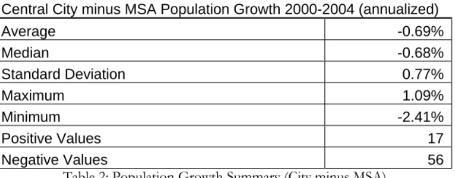
Subtracting the MSA population annualized growth rate from the central city’s rate gives the city’s relative over-performance/under-performance compared to its associated MSA. The resulting population growth dependent variable shows whether people are moving into or out of cities, relatively speaking. First, a summary of the results of this transformation of seventy three city/MSA pairs is shown below in Table 2. The detailed results can be found in Appendix II.

Central City minus MSA Population Growth 2000-2004 (annualized)

Average -0.69% Median -0.68% Standard Deviation 0.77% Maximum 1.09% Minimum -2.41% Positive Values 17 Negative Values 56

Table 2: Population Growth Summary (City minus MSA)

In this summary, the measures of central tendency indicate that most cities are lagging their MSAs in population growth. In fact, only 23% of cities in the sample grew faster, on an annualized basis, than their associated MSA. This result confirms Sohmer and Lang’s 2005 findings. Raleigh, NC leads the relative city population growth with a 1.09% advantage while Washington, DC lagged its MSA by 2.41%.

(32)

Section 5.1.2 Regression Results and Discussion

Regressing relative city/MSA population growth on twelve independent variables results in a of 0.46. Of the independent variables, six exhibit t-stats with absolute values greater than 1.0:

2 R

1. Average Daily Traffic Per Freeway Lane Mile: With a t-stat of -3.24, there is only a 0.2% chance that this variable has no observable relationship to relative city population growth, meaning that this coefficient has significant explanatory power. The

coefficient of 6

1.082 10−

− × implies that for every 1,000 vehicle increase in average daily traffic per freeway lane mile, the city population growth rate is 0.11% lower relative to its MSA. Intuitively, this makes sense as it would appear that higher traffic on the freeways of an MSA implies that people are likely to be living in a different city than their place of work. Additionally, this rejects the hypothesis that higher traffic which increases the cost of inter-city travel should be postively correlated to relative city growth. Also, the results do not support the notion that high-traffic MSAs will see residents flocking into central city residences to avoid commuting.

2. City as Proportion of MSA (Population): With a t-stat of 1.13, this variable has marginal explanatory power. However, the coefficient of 0.007 is at least in the right

direction. Recall that on average, cities lagged MSAs in population growth so therefore as cities become essentially the same as MSAs by approaching one, the deficit decreases.

3. Combined Degree Days: A t-stat of -1.22 with a coefficient of , while not having strong explanatory power, at least matches the direction of the hypothesis. It appears that as cities become more inclement, they do worse

compared to their MSAs. Intuitively, this makes sense as people in harsher climates

7

8.223 10−

(33)

are less willing to get out of their cars and embrace the walking/transit required in denser central city living.

4. Crime Index: With a t-stat of -1.44, there’s a 15% chance that Crime Index has no observable relationship to relative city population growth. Therefore Crime Index moderately explains the variance in relative city population growth. The coefficient of -0.0024 implies that for every unit increase in the Crime Index, the city

population growth rate lags its MSA by 0.24%. Again, intuitively this makes sense and confirms the hypothesis because it implies that cities that higher crime rates do not attract residents, especially larger households such as families, as quickly as the safer suburbs.

5. Major River Dummy: With a t-stat of -1.37 on a coefficient of -0.0022, it appears that this moderate explanatory power variable counters the hypothesis. For some reason, a city’s location next to a major river correlates with less population growth relative to its MSA. Potentially, the fact that many of the cities near major rivers in the US are used for industrial traffic and historically industry located near these rivers, residents often prefer suburbs in those cities.

6. Roadway Miles per 10,000 Population: While this explanatory variable has a strong t-stat of -2.84, the coefficient is only -.0003, implying that every additional roadway mile per 10,000 population correlates to only 0.03% lag in city population growth. For the sample, the average RM per 10,000 stands at 43.0 with a standard deviation of 12.0, therefore while roadway miles has strong explanatory power, the effect is not overpowering. Intuitively, the direction of correlation makes sense and provides supporting evidence, however weak, for the hypothesis and Duany’s assertion that roadway construction promotes central city population drain (2000).

(34)

Observations 73

Table 3: City minus MSA Population Growth Regression Results

Regression Statistics

Multiple R 0.674989051

R Square 0.455610219

Adjusted R Square 0.335659929

Standard Error 0.006305528

Independent Variable Coefficients Standard Error t Stat P-value Lower 95% Upper 95%

Intercept 0.033138941 0.036427667 0.909718997 0.366610772 -0.039727241 0.106005123 Average Daily Traffic Per FLM -1.08153E-06 3.33728E-07 -3.240749347 0.001946886 -1.74908E-06 -4.13973E-07 Average Household Size 0.001323472 0.007867607 0.168217872 0.866977642 -0.014414085 0.017061029 City as proportion of MSA (Population) 0.00700079 0.006184478 1.131993726 0.262140939 -0.005370007 0.019371588 Combined Degree Days -8.22324E-07 6.70639E-07 -1.226179976 0.224921624 -2.1638E-06 5.19154E-07 Crime Index -0.002425293 0.001683045 -1.441014946 0.154779116 -0.005791884 0.000941298 LargeLake/Ocean Dummy 0.000263464 0.001893493 0.139141813 0.889804075 -0.003524086 0.004051014 Major River Dummy -0.002278904 0.001658247 -1.374285669 0.174464842 -0.005595891 0.001038082 Median Age -0.000166257 0.000479697 -0.34658684 0.730114309 -0.001125794 0.000793281 Median Age of Housing Unit -6.32037E-05 9.02042E-05 -0.700673475 0.486215207 -0.000243639 0.000117232 Median HH Income -1.85856E-08 1.82948E-07 -0.101589391 0.919421339 -3.84536E-07 3.47365E-07 0.039604504 Prop. w/ Bachelors or Greater -0.001561947 0.020580161 -0.075895752 0.939754537 -0.042728397

(35)

2 R

6

1.125 10

Table 4 on the next page details the complete results of the truncated dataset regression: Because the OLS regression method assumes no outliers, removal of data with significant residuals will likely improve the model’s explanatory power. By removing the two data points that have standardized residuals with an absolute value greater than 1.96 and regressing the resulting truncated dataset, the improves to 0.51. The explanatory power of five of the aforementioned variables improves and one declines. The changes include:

6. Roadway Miles per 10,000 Population: T-stat improves to -2.89 and the coefficient remains the same at 0.003.

5. Major River Dummy: The t-stat degrades significantly to -0.78 and the coefficient nearly halves to -0.0011. This variable no longer crosses the established threshold and therefore cannot be reliably analyzed.

4. Crime Index: T-stat improves to -1.45 but at the same time, the coefficient decreases in magnitude to -0.0022

1. Average Daily Traffic Per Freeway Lane Mile: T-stat improves to -3.71 and the coefficient increases in magnitude to − × −

7

9.261 10 .

3. Combined Degree Days: T-stat for this independent variable goes to -1.54 with an increase in coefficient magnitude to

2. City as Proportion of MSA: T-stat improves to 1.32 and coefficient gains very little magnitude to 0.0074.

−

(36)

Regression Statistics Multiple R 0.71502438 R Square 0.511259864 Adjusted R Square 0.410141215 Standard Error 0.005597343 Observations 71

Intercept 0.009251986 0.033128946 0.279271965 0.78102957 -0.057062803 0.075566775 Average Daily Traffic Per FLM -1.12536E-06 3.03128E-07 -3.712486873 0.000462456 -1.73214E-06 -5.18583E-07 Average Household Size 0.00698786 0.007202741 0.970166776 0.335991901 -0.007429993 0.021405714 City as proportion of MSA (Population) 0.00742244 0.005637647 1.316584752 0.193156803 -0.003862536 0.018707416 Combined Degree Days -9.26054E-07 6.01068E-07 -1.540681254 0.128832967 -2.12922E-06 2.77114E-07 Crime Index -0.002193125 0.001507773 -1.454546238 0.15118561 -0.00521126 0.00082501 LargeLake/Ocean Dummy 0.000851645 0.00170186 0.500420193 0.618672838 -0.002554998 0.004258288 Major River Dummy -0.001180172 0.001509049 -0.782063042 0.43735868 -0.004200863 0.001840519 Median Age 5.58204E-05 0.000433317 0.128821038 0.897944931 -0.000811558 0.000923199 Median Age of Housing Unit -2.99706E-05 8.21508E-05 -0.364824962 0.71656898 -0.000194413 0.000134472 Median HH Income -8.66978E-08 1.65485E-07 -0.523899839 0.602344517 -4.17953E-07 2.44557E-07 Prop. w/ Bachelors or Greater 0.00651672 0.018934886 0.344164711 0.731967124 -0.031385572 0.044419011 Roadway Miles per 10,000 population -0.000250767 8.67691E-05 -2.890050678 0.005410321 -0.000424455 -7.70799E-05

(37)

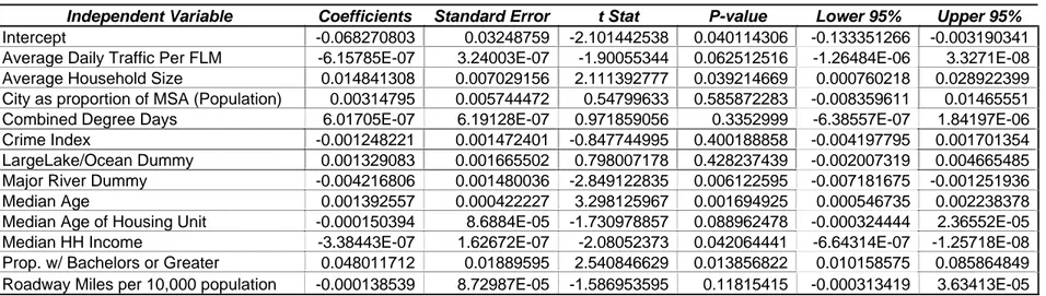
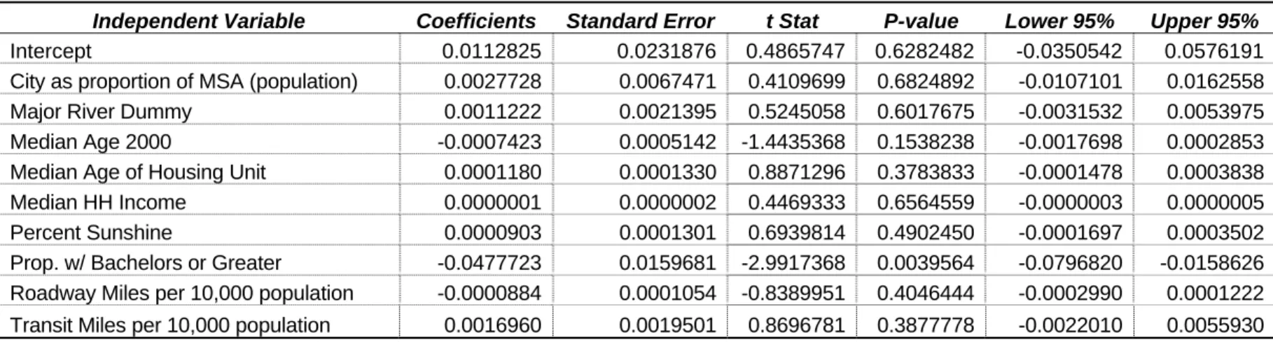
The relative city population growth regression results confirm some hypotheses while rejecting others. Specifically, Crime Index, Combined Degree Days and Roadway Miles per 10,000 Population were confirmed to be negatively correlated with relative city growth performance while the prediction for Combined Degree Days appeared to be weakly confirmed. While City Share of MSA does not appear to be significant, the coefficient is in the correct positive direction. More interestingly, household size, proximity to water amenities and transit miles showed no significant relationship to the population growth metric.

(38)

Section 5.2 City minus MSA Housing Unit Growth (2000-2004 Annualized)

Housing Unit Growth Hypothesis – The hypotheses for relative housing unit growth mirrors the

population growth predictions. Educational attainment should be positively correlated with relative housing unit growth while crime rate and household size will have the opposite relationship. For environmental variables, combined degree days, a proxy for climatic adversity, will have a negative relationship while proximity to water amenities should be positively correlated to relative city housing unit growth. And finally, for transportation variables, I expect relative city housing unit growth to occur most strongly where difficult inter-city travel combines with efficient intra-city travel. Again, that implies that transit miles will trend in the same direction as relative city housing unit growth while roadway miles will exhibit a negative correlation.

Section 5.2.1 Dependent Variable Transformation

Subtracting the MSA annualized housing unit growth rate from the central city’s rate gives the city’s relative over-performance/under-performance compared to its associated MSA. The resulting dependent variable shows whether housing units are being added to cities faster than to MSAs. This difference in growth rates may or may not match the population growth metric for each city/MSA pair. For example, if housing units are growing faster in cities but the people moving in are singles displacing families, population growth for that city/MSA pair may favor the MSA. First, a summary of the results of this transformation of seventy three city/MSA pairs are shown on the next page in Table 5. The detailed results can be found in Appendix II.

(39)

Central City minus MSA Housing Unit Growth 2000-2004 (annualized) Average -0.60% Median -0.69% Standard Deviation 0.84% Maximum 1.60% Minimum -2.38% Positive Values 14 Negative Values 59

Table 5: Housing Unit Growth Over/Under Performance Summary

In comparison to the relative city population growth outcome variable, the summary statistics for City minus MSA Housing Unit Growth show that average relative city housing unit growth has a smaller negative magnitude and higher maximum and minimum values. So while the number of city/MSA pairs with positive housing unit growth metrics lags the count for positive population growth metric values, it appears that overall, more housing units are being added to cities than population. The maximum value occurs in Bakersfield, CA with 1.60% relative city housing unit growth while Las Vegas city lags its MSA by 2.38%. Growth in housing units more accurately approximates growth in households since each household demands a housing unit while each person may not. The dependent variable summary statistics imply shrinkage in average household size. This provides support for earlier studies that assert that families are moving out of central cities while singles and empty nesters are moving in.

(40)

Section 5.2.2 Regression Results and Discussion

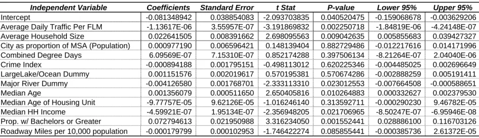
Regressing relative city/MSA housing unit growth on the same twelve independent variables results in a of 0.48. Of the independent variables, seven exhibit t-stats with absolute values greater than 1.0:

2 R

1. Average Daily Traffic Per Freeway Lane Mile: With a t-stat of -3.19, this transportation statistic has significant explanatory power. The coefficient of

combined with the higher t-stat implies that this variable has a more significant and stronger effect on housing unit growth than on population growth. This confirms the stated hypothesis. Again, the results do not support the notion that high-traffic MSAs will see households flocking into central city residences to avoid commuting.

7

4.599 10−

− ×

2. Average Household Size: With a t-stat of 2.69 and a coefficient of 0.022, average household size shows significant positive correlation with housing unit growth. Note that the average value for household size in our sample is 2.48 with a standard deviation of only 0.23, meaning that while the effect is significant, there is not much deviation in terms of actual values. Despite this low effect, this relationship runs counter to the belief that a higher proportion of empty nesters and echo boomers (who generally have smaller household sizes than families) will result in higher relative city housing unit growth. Alternatively and plausibly, it could be that cities that currently have many larger family households are experiencing net

out-migration of families and the smaller households that replace them require

additional housing units to provide for the shrinking average household size. This result does not confirm the hypothesis.

3. Major River Dummy Variable: Surprisingly, proximity to a major river does not appear to correlate with higher relative central city housing unit growth rates. With a t-stat of -2.33 and a coefficient of -0.004, a city close to a major river appears to

(41)

grow in housing units 0.4% slower than its MSA. This runs counter to the stated hypothesis.

4. Median HH Income: Higher income appears to correlate with lower relative central city housing unit growth rates. A t-stat of -2.36 with a coefficient of 6

7.283 10−

− ×

shows strong significance with a reasonably strong effect. The income data has an average of $37,164 and a standard deviation of $7,626 showing that considerable variation in household income exists across the sample. This provides support to the argument that echo boomers and to a lesser extent, retiring baby boomers are moving back into cities because in general, younger professionals and older retirees earn less than their middle aged counterparts. This is inconclusive, however because it could also imply that cities that have high poverty rates do not attract building. Therefore, additional research is necessary to determine exact income distribution across the sample cities.

5. Median Age: A t-stat of 2.65 and a coefficient of 0.0013 imply strong explanatory power yet weak effect. The summary statistics for median age data show that with an average age of 33 and a standard deviation of only 2 years, there is not much variation across the sample cities.

6. Median Age of Housing Unit: With a t-stat of -1.02 and a coefficient of 5

9.778 10−

− × ,

this variable has marginal explanatory power. It is however, interesting in that cities with older existing stock do worse, indicating that perhaps the redevelopment of older buildings is not occurring at a very fast rate. It could also be a proxy for complexity of zoning laws, as more strict cities may have older housing stock as a result of their Byzantine laws.

7. Proportion of Population 25+ with Bachelors or Greater: With a very strong t-stat of 3.31 and a coefficient of 0.07, higher education correlates significantly and strongly with higher relative central city growth. The data has an average of 26% and a standard

(42)

deviation of 8%, showing reasonably large variation in sample data. This result provides support for Birch’s 2005 assertion and the hypothesis that highly educated people are moving back downtown.

8. Roadway Miles Per 10,000 Population: Despite having a strong t-stat of -1.74, this variable’s coefficient is only -0.0001. Additionally, the 95% confidence interval for the coefficient includes zero. So while roadway miles appears to have a negative correlation with housing unit growth, it does not respond as strongly as it did with population growth. However, assuming the negative correlation holds, however weak, it provides additional support for Duany’s assertion that roadway

construction causes flight from the central city (2000).

(43)

Table 6: City minus MSA Housing Unit Growth Regression Results Regression Statistics Multiple R 0.689292 R Square 0.475123 Adjusted R Square 0.370148 Standard Error 0.00667 Observations 73

Intercept -0.081348942 0.038854083 -2.093703835 0.040520475 -0.159068678 -0.003629206 Average Daily Traffic Per FLM -1.13617E-06 3.55957E-07 -3.191869832 0.002250718 -1.84819E-06 -4.24148E-07 Average Household Size 0.022641505 0.008391662 2.698095563 0.009042635 0.005855683 0.039427327 City as proportion of MSA (Population) 0.000977190 0.006596421 0.148139404 0.882729486 -0.012217616 0.014171996 Combined Degree Days 6.09569E-07 7.15310E-07 0.852174288 0.397506134 -8.21264E-07 2.04040E-06 Crime Index -0.000894188 0.001795151 -0.498113012 0.620225346 -0.004485025 0.002696649 LargeLake/Ocean Dummy 0.001151576 0.002019617 0.570195381 0.570674286 -0.002888259 0.005191411 Major River Dummy -0.004126580 0.001768701 -2.333113310 0.023012553 -0.007664508 -0.000588651 Median Age 0.001356079 0.000511650 2.650405816 0.010264883 0.000332627 0.002379530 Median Age of Housing Unit -9.77757E-05 9.62126E-05 -1.016246140 0.313592711 -0.000290230 9.46782E-05 Median HH Income -4.59921E-07 1.95134E-07 -2.356948205 0.021706965 -8.50247E-07 -6.95946E-08 Prop. w/ Bachelors or Greater 0.072794613 0.021950988 3.316234050 0.001552441 0.028886100 0.116703126 Roadway Miles per 10,000 population -0.000179799 0.000102953 -1.746422274 0.085855441 -0.000385736 2.61372E-05

(44)

2 R

Table 7 on the next page details the complete results of the truncated dataset regression: Removing the four outliers with standardized residuals greater than 1.96 or less than -1.96 results in a new regression where improves to 0.54. The explanatory power of three of the aforementioned variables improves. The changes include:

4. For five variables (Average Daily Traffic per Freeway Lane Mile, Average Household Size,

Median Household Income, Proportion with Bachelor’s or Greater and Roadway Miles) the

regression on the truncated dataset resulted in lower t-stats, but all remain above the t-stat threshold of 1.0.

3. Median Age of Housing Unit: The t-stat on median age of HU increased to -1.73 with a coefficient of 0.0002. While significance is reasonably high, the coefficient value does not imply much effect.

2. Median Age: T-stat improves to 3.30 with very little change in coefficient. 1. Major River Dummy Variable: T-stat improves to -2.85 with very little change in

(45)

Regression Statistics Multiple R 0.732276364 R Square 0.536228673 Adjusted R Square 0.436849103 Standard Error 0.005437345 Observations 69

Intercept -0.068270803 0.03248759 -2.101442538 0.040114306 -0.133351266 -0.003190341 Average Daily Traffic Per FLM -6.15785E-07 3.24003E-07 -1.90055344 0.062512516 -1.26484E-06 3.3271E-08 Average Household Size 0.014841308 0.007029156 2.111392777 0.039214669 0.000760218 0.028922399 City as proportion of MSA (Population) 0.00314795 0.005744472 0.54799633 0.585872283 -0.008359611 0.01465551 Combined Degree Days 6.01705E-07 6.19128E-07 0.971859056 0.3352999 -6.38557E-07 1.84197E-06 Crime Index -0.001248221 0.001472401 -0.847744995 0.400188858 -0.004197795 0.001701354 LargeLake/Ocean Dummy 0.001329083 0.001665502 0.798007178 0.428237439 -0.002007319 0.004665485 Major River Dummy -0.004216806 0.001480036 -2.849122835 0.006122595 -0.007181675 -0.001251936 Median Age 0.001392557 0.000422227 3.298125967 0.001694925 0.000546735 0.002238378 Median Age of Housing Unit -0.000150394 8.6884E-05 -1.730978857 0.088962478 -0.000324444 2.36552E-05 Median HH Income -3.38443E-07 1.62672E-07 -2.08052373 0.042064441 -6.64314E-07 -1.25718E-08 Prop. w/ Bachelors or Greater 0.048011712 0.01889595 2.540846629 0.013856822 0.010158575 0.085864849 Roadway Miles per 10,000 population -0.000138539 8.72987E-05 -1.586953595 0.11815415 -0.000313419 3.63413E-05

(46)

The relative city housing unit growth regression results confirm some hypotheses while rejecting others. Specifically, Roadway Miles per 10,000 Population was weakly confirmed to be negatively correlated to relative city growth performance while Proportion of Bachelor’s exhibited the predicted positive correlation in a more significant manner. The results for the Average Household Size and the Major River Dummy Variable, however, ran counter to the prediction. Interestingly, Age of Housing Unit exhibited negative correlation to our dependent variable, indicating that redevelopment is not occurring very quickly. Again, while City Share of MSA does not appear to be significant, the coefficient is in the correct positive direction. The other water amenity variable, Large Lake / Ocean Dummy Variable showed no significant relationship to the dependent variable and neither did the proxy for climatic adversity, namely Combined Degree Days.

(47)

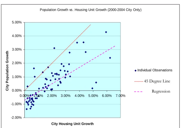
Section 5.3 Housing Unit Growth vs. Population Growth (2000-2004 City Only) Reviewing the summary statistics of the two previous dependent variables, City Population Growth and City Housing Unit Growth (relative to the MSA), reveals that average housing unit growth outpaces average population growth. Additionally, both the minimum and maximum observations of the housing unit growth dependent variable are higher than the corresponding population growth observations. This comparison of measures of central tendency, however, does not allow observation of individual data points and could be skewed by a few extreme outliers.

By plotting Annual City Housing Unit Growth against Annual City Population Growth and drawing a 45 degree line, we can observe the overall pattern with better resolution than can be provided by simple summary statistics.9_{An observation that lies on}

the 45 degree line has equivalent housing unit and population growth. Any deviation from this line would indicate likely changes in household composition. The resulting plot can be seen below in Figure 3 and the complete data table is included in Appendix III.

9_{Note that the two variables represent City growth rates and not the linear difference between city and MSA growth rates} as before.

(48)

Population Growth vs. Housing Unit Growth (2000-2004 City Only) -2.00% -1.00% 0.00% 1.00% 2.00% 3.00% 4.00% 5.00% 0.00% 1.00% 2.00% 3.00% 4.00% 5.00% 6.00% 7.00%

City Housing Unit Growth

C it y P o pu la ti on Gr o w th Individual Observations 45 Degree Line Regression

Figure 3: Population vs. Housing Unit Growth

In the figure above, the finely dotted line represents linear growth in both housing units and population. Of the seventy three cities, only Wichita, Fresno and New York City lie very near or on the forty five degree line.10_{Additionally, Fort Wayne, Riverside (CA) and}

Los Angeles lie above the linear growth line, implying that population has outpaced housing unit growth in these cities. The majority of cities lie below the forty five degree line with a large cluster exhibiting zero to one percent housing unit growth with zero to negative one percent population growth.

Examining the majority of cities again, we can clearly see that they appear to arrange themselves in a near-linear manner with a slightly negative y-intercept. Performing a

10_{Only Wichita, with 1.33% population and 1.33% housing unit growth, is exactly on the line. Fresno has 1.72% and} 1.71% growth and New York City has 0.22% and 0.30% growth, respectively.

(49)

univariate regression yields a model with a 2

R of 0.61, a y-intercept of -0.74% and a

coefficient estimate of 0.690 with a very high t-stat of 10.56. The least squares fit line appears on Figure 3 as a dashed line. With a slope of less than one, it appears that the model predicts that as housing growth accelerates, the disparity between HU growth and population growth grows even larger. This could derive from various reasons. Potentially, cities with very rapid housing unit growth have very aggressive redevelopment initiatives and therefore have development far outpacing what would occur in an unadulterated market. An innocuous explanation is that cities with a large disparity between housing unit and population growth could simply be experiencing greater shrinkage in household size due to families moving out and singles moving in. Cynically, perhaps the cities with significant development activity attract not residents, but frenzied investors looking to gamble with downtown condominiums rather than Internet stocks.11

11_{Not surprisingly, Las Vegas appears towards the upper right, with HU growth of 4.46% on only 2.83% population} growth.