HAL Id: hal-03042941
https://hal.archives-ouvertes.fr/hal-03042941
Submitted on 7 Dec 2020
HAL is a multi-disciplinary open access
archive for the deposit and dissemination of sci-entific research documents, whether they are pub-lished or not. The documents may come from teaching and research institutions in France or abroad, or from public or private research centers.
L’archive ouverte pluridisciplinaire HAL, est destinée au dépôt et à la diffusion de documents scientifiques de niveau recherche, publiés ou non, émanant des établissements d’enseignement et de recherche français ou étrangers, des laboratoires publics ou privés.
Thomas Grebel, Lionel Nesta
To cite this version:
Thomas Grebel, Lionel Nesta. Competition and private R&D investment. PLoS ONE, Public Library of Science, 2020, 15, �10.1371/journal.pone.0232119�. �hal-03042941�
RESEARCH ARTICLE
Competition and private R&D investment
Thomas Grebel1☯¤a, Lionel NestaID2,3,4☯¤b*
1 TU Ilmenau, Economics Department, Ilmenau, Germany, 2 Groupe de Recherche en Droit, Economie,
Gestion, Universite´ Cote d’Azur, France, 3 SciencesPo, OFCE, Paris, France, 4 SKEMA Business School, Sophia-Antipolis, France
☯These authors contributed equally to this work.
¤a Current Address: TU Ilmenau, Economics Department, Ilmenau, Germany ¤b Current Address: 250 rue Albert Einstein, Sophia-Antipolis, France *[email protected]
Abstract
We investigate the determinants of the sign of Research and Development reaction func-tions of rival firms. Using a two-stage n-firm Cournot competition game, we show that this sign depends on four types of environments in terms of product rivalry and technology spill-overs. We test the predictions of the model on the world’s largest manufacturing corpora-tions. Assuming that firms make R&D investments based on the R&D effort of the
representative rival company, we develop a dynamic panel data model that accounts for the endogeneity of the decision of the rival firm. Empirical results thoroughly corroborate the validity of the theoretical model.
Introduction
A striking outcome of the recent paper by [1] is that the relationship between a firm’s own R&D and that of a product market rival is ambiguous. The slope of the R&D reaction function, whether positive or negative, depends on how the research effort by the rival company affects the profitability of the firm’s own R&D. Our intuition is that when studying R&D reaction functions, one must first determine the context within which any two firms compete in terms of technology spillovers and product market rivalry. This mix determines whether the R&D investments by two companies are strategic complements or substitutes.
The question of the complementarity or substitution of R&D investments in the presence of spillovers by firms is crucial. Due to positive externalities, such investments are typically seen as strategic substitutes [2,3,4]. More recently, Strandholm et al. [5] show that the social welfare effects of policies are crucially dependent on the presence of technology spillovers. However, these contributions implicitly assume that firms are rivals on the product market. Instead, imagine that firms sell complementary products. Our intuition is that an increase in a firm’s own R&D may very well encourage its strategic complement to also increase its research efforts. A better understanding of such mechanisms would help to design better R&D policies supporting private research [6].
This article develops a two-stage non-cooperative Cournot model that reconciles the views that technology spillovers may either impede or conversely motivate firm R&D investments. A a1111111111 a1111111111 a1111111111 a1111111111 a1111111111 OPEN ACCESS
Citation: Grebel T, Nesta L (2020) Competition and
private R&D investment. PLoS ONE 15(5): e0232119.https://doi.org/10.1371/journal. pone.0232119
Editor: Ana Espinola-Arredondo, Washington State
University, UNITED STATES
Received: December 1, 2019 Accepted: April 7, 2020 Published: May 27, 2020
Peer Review History: PLOS recognizes the
benefits of transparency in the peer review process; therefore, we enable the publication of all of the content of peer review and author responses alongside final, published articles. The editorial history of this article is available here:
https://doi.org/10.1371/journal.pone.0232119
Copyright:© 2020 Grebel, Nesta. This is an open access article distributed under the terms of the
Creative Commons Attribution License, which permits unrestricted use, distribution, and reproduction in any medium, provided the original author and source are credited.
Data Availability Statement: Data cannot be
shared publicly because we use private Compustat data. Such data are available from the Wharton Research Data Service (contact via https://wrds-www.wharton.upenn.edu/) for researchers who meet the criteria for access to confidential data.
key assumption of the model is that the goods produced by the two firms are imperfect substi-tutes [7,8]. The rationale is straightforward. If firms do business in complementary or inde-pendent markets, they do not compete in output. Technology spillovers may then be beneficial or harmless to both companies because they do not reduce a firm’s market size. Conversely, if products are close substitutes, technology spillovers may enter the production function of the rival company. Whether firms reap profits from their research efforts depends on the degree of knowledge spillovers and of product substitution. It is this mix between technology spillovers on the one hand and product market competition on the other that will determine whether R&D investments between any two companies are complements or substitutes.
This article also develops an empirical version of the R&D reaction function and applies it to data on the world’s largest companies. The combination of patent data from the USPTO and financial information from Compustat of 308 companies allows us to determine the degree of technological spillovers and of product substitution for any dyad of firms. Because companies cope with an array of competitors, we assume that firms makeoblivious R&D
investments based on the R&D decision of therepresentative rival company. This assumption
allows us to empirically determine the sign of the R&D reaction function. Pre-sample mean panel data models accounting for the endogeneity of the R&D decision by the rival company corroborate the theoretical predictions.
The originality of this article is threefold. First, on the theoretical side, we concentrate exclusively on the sign of the R&D reaction function. By doing so, we show that the sign is fully determined by the degree of technology spillover and product market rivalry. Second, on the empirical side, all contributions treat technology spillovers and/or product market rivalry as determinants of innovation, profitability, or market value. Instead, we consider technology spillovers and product market rivalry as the elements that provide a context within which two rival firms determine their level of R&D efforts. Third, we develop an empirical version of the theoretical R&D reaction function that accounts for the simultaneity of such decisions using the generalized method of moments. Our results are consistent with the theoretical framework, implying that contrary to the usual wisdom, spillovers may spur firm R&D investments.
Section (1) introduces the model. Section (2) investigates the conditions that determine the positive and negative correlations between the firms’ process R&D. Sections (3) and (4) pres-ent the empirical protocol and discuss the results. Section (5) concludes.
1 The model
The model builds on the contribution by De Bondt Veugelers [7]. We considern firms that
produce differentiated goods in quantityqiwithi = {1, 2, . . ., n}, with the numeraire good m. As in Lin and Saggi [8], who develop a duopoly model along previous work such as by Dixit [9] and Vives [10] substantiating entry barriers and discussing the role of information and competitive advantages, we employ a representative consumer’s utility function associated with the consumption of differentiated goods. The utility function we use takes a quadratic form as in Amir et al. [11]:
UðqÞ ¼ aq 1
2qSq þ m ð1Þ
witha as a positive n–vector and S as a symmetric n × n–matrix with a diagonal of value 1 and σ else. Parameter σ represents the degree of substitution between products. Unlike Lin and
Saggi [8] and identical to Bondt Veugelers [7], we allowσ to be either negative or positive: −1
�σ � 1. A positive value for σ implies that products are substitutive (i.e., low product
differen-tiation), whereas a negative value entails complementarity between goods. This utility function
The patent data and all programmes underlying the results presented in the study are available through harvard Dataverse from the following DOI:https:// dataverse.harvard.edu/dataset.xhtml?persistentId= doi:10.7910/DVN/IQD9HT.
Funding: The authors received no specific funding
for this work.
Competing interests: The authors have declared
suggests both a preference for variety—because of its quadratic terms—and a taste for product differentiation—because of the negative effect ofσ on consumer utility.
The inverse demand function derived from the quadratic utility function from above leads to: pi ¼a bqi sb X j6¼i qj ð2Þ withqiþ Pn
i6¼1qi¼Q < a=b. Note that if σ > 0 (resp. σ = 1), the products are (resp. perfect)
substitutes, implying that firms compete in an oligopoly market. If insteadσ < 0, products are
complementary: an increase in the demand for one product increases the demand for comple-mentary products, leading to an increase in its price. Ifσ = 0, products are entirely unrelated,
and firms operate as monopolists in different markets. Hence, an increase in the degree of product differentiation (i.e., a decrease inσ), denotes an outward shift of the demand curve for
firms.
Firms face constant marginal costA, which can be reduced by means of process R&D xi. As in D’aspremont and Jacquemin [12], firms face externalities in process R&D, depicted by parameterβ which indicates the spillovers from remaining firms’ process R&D. The marginal cost of production is computed as
Ci ¼A xi b
X
j6¼i
xj ð3Þ
where 0 <A < a and xi+β∑j6¼ixj<A. As in De Bondt and Veugelers [7], we assume
−1 < β < 1. Positive externalities (β > 0) imply positive R&D spillovers due to a lack of appro-priability. The case for negative externalities (β < 0) is admittedly more subtle, but they may stem from factor market imperfections which increase rival firms’ marginal cost. We mainly consider skill-biased technical change, which, by increasing the demand for skilled labor, increase their equilibrium wage for the entire population of firms. Hence, the mathematical continuum of the interval forβ should not conceal the difference in nature that exists between a positiveβ, which is mainly technological, and a negative β, which is mainly pecuniary.
We assume convex costs in process R&D investment, gx2
i=2, with efficiency parameter
γ > 0. The profit function reads:
pqi ¼½pi Ci�qi
g 2x
2
i ð4Þ
wherepiandCiare defined by Eqs (2) and (3), respectively.
Altogether, the structure of the game is as follows. In the first stage, firms choose optimal R&D investments. In the second stage, firms decide on optimal production quantity. The firm’s maximization problem is solved by backward induction. Therefore, we first consider the output stage and thereafter the R&D stage.
Output stage
Firms choose optimal output levels to maximize profits. The first-order condition with respect toqireads:
a 2bqi sbðQ qiÞ Ci¼ 0; ð5Þ
i = 1, ‥, n gives na bð2 þ ðn 1ÞsÞQ CS¼ 0 withCS¼Pn i¼1Ciand @ 2 pqi i =@qi
2¼ 2 > 0 8 b > 0, q�determining a maximum. This
leads to total output in equilibrium
Q�
¼ na C
S
bð2 þ ðn 1ÞsÞ: ð6Þ InsertingEq (6)intoEq (5)leads to equilibrium output of the representative firm:
q�
i ¼
ð2 sÞa ð2 þ ðn 2ÞsÞCiþ sC i
bðs 2Þððn 1Þs þ 2Þ ð7Þ
withC−i=CS− Ci. Equilibrium profit can then be written as:
pq�i ¼a bq�i bs Xn j6¼i q� j CiÞq � i g 2x 2 i ð8Þ
Assuming n = 2 and settingσ to unity yields equilibrium output q�
i and profit p q�
i , identical
to d’Aspremont and Jacquemin [12]. Settingβ to zero instead yields optimal output q�
i and
profit pq�i identical to Lin and Saggi [8].
Process R&D stage
The first-order condition inEq (5)is equivalent to ðpi CiÞ ¼bq
�
i. Hence, the reduced form
of the profit function in the process R&D stage is: pq�i ¼bðq� iÞ 2 g 2x 2 i ð9Þ
To obtain the optimal level of process R&D, the respective first-order condition at this stage reads: 2bq� i @q� i @xi gxi¼ 0
FromEq (3), we deduce that a one unit change inxichanges marginal costsCiby minus one unit, i. e. @Ci/@xi=−1. As the symmetry assumption of firms also holds at the R&D stage, we can state that @q�
i=@xi¼ k, for alli = 1, . . ., n. Using this information together witchEq (7),
we can derive k ¼ @q � i @Ci bðn 1Þ@q � i @Cj ; for j 6¼ i ð10Þ ¼ 2 þ ðn 2Þs bð2 sÞð2 þ ðn 1ÞsÞ bðn 1Þ s bð2 sÞð2 þ ðn 1ÞsÞ ð11Þ ¼2 s þ ðn 1Þsð1 bÞ bð2 sÞð2 þ ðn 1ÞsÞ : ð12Þ
Summing over all first-order conditions at R&D stage yields the first-order condition:
wherex�denotes the equilibrium value of firm-level R&D. Inserting the marginal cost function CiinEq (3)intoEq (6), we obtain Q� ¼nða AÞ þ nð1 þ ðn 1ÞbÞx � bð2 þ ðn 1ÞsÞ :
Now, we can calculate firm-level R&D, pluggingQ�
andκ intoEq (13). This renders equi-librium R&D
x� ¼ 2ð2 s þ ðn 1Þsð1 bÞÞða AÞ
gbð2 sÞð2 þ ðn 1ÞsÞ2 2ð2 s þ ðn 1Þsð1 bÞÞð1 þ ðn 1ÞbÞÞ ð14Þ In the duopoly case (n = 2), this reduces to
x� ¼ ða AÞð2 bsÞ b 2gð2 sÞð2 þ sÞ 2 ð2 bsÞð1 þ bÞ : ð15Þ
Note that this result is in line with the model from d’Aspremont Jacquemin [12]. By setting
σ = 1, optimal process R&D investment (x�) corresponds to the non-cooperative version of
their model.
At this stage, in previous contributions such as d’Aspremont Jacquemin [12], Bondt Veuge-lers [7], Lin and Saggi [8] and Strandholm et al. [5], a discussion of the welfare effects of rivalry in R&D investments and on product markets follows. We provide such an analysis of the wel-fare effect of product rivalry and technology spillovers in Appendix (A). However, our conten-tion is that product rivalry and the presence of technology spillovers modify the firms’
incentives to invest in research activities. Next Section focuses on this particular issue.
2 R&D reaction functions in the
β
-
σ
space
As we focus on strategic R&D investment behavior, we now investigate the reaction function
Ri(xj) with varying values ofσ and β while assuming symmetric reactions with uniform param-etersa, A, b, γ, β and σ. This implies that firm i responds to the R&D investments of the
remaining (n–1) firms. In the following steps, we derive the R&D reaction function Ri(xj): insertingq�fromEq (7)intoEq (9), replacingC
i=A − xi− β(n − 1)xj, andC−i= (n − 1)A − (n
− 1)βxi− (1 − (n − 2))∑j6¼ixj, yields the full form of the R&D-stage profit funtion:
pq� ðxi;xjÞ ¼ ððs 2Þða AÞ þ xiðsðbðn 1Þ n þ 2Þ 2Þ þ ðn 1Þðs 2bÞxjÞ 2 bðs 2Þ2ððn 1Þs þ 2Þ2 gx2 i 2 Setting the first derivative of this profit function to zero and solving forxileads to the fol-lowing reaction function:
RiðxjÞ :xi¼ Cð2 sÞða AÞ Cðn 1Þðs 2bÞxj ð16Þ
with C ¼b2gðs 2Þ2ðð2ð2 sþðb ðb 1Þn 1Þsþ2Þ2 2ðsðbð1n 2ÞÞnÞþn 2Þþ2Þ2. The equation is linear inxjand describes the best
response of firmi to the average optimal R&D investments of the representative competitor
(note, in equilibrium:xj=x�).
Equivalently, we assume, below in our empirical exercise, that firms do not react in their R&D investment decisions to a single competitor but rather to a representative competitor. To align the model to our empirical design, we also reduce our model to the casen = 2. The
corresponding R&D reaction function thus reads: RiðxjÞ :xi ¼ 2ða AÞð2 sÞð2 bsÞ=bð4 s2Þ2 2ðbs 2Þ2 bð4 s2Þ2 g þ2ð2b sÞðbs 2Þ=bð4 s 2Þ2 2ðbs 2Þ2 bð4 s2Þ2 g xjð17Þ
withi, j = 1, 2 and i � j. The denominators of the two summands inEq (17)reflect the second-order condition in the R&D stage and must be negative. Observe thatEq (17)is a linear func-tion of the formxi=α + ωxj. Computingdxi/dxjyields:
dxi dxj ¼ o ¼ 2ða AÞð2 bsÞð2b sÞ=bð4 s 2Þ2 2ð2 bsÞ2 bð4 s2Þ2 g : ð18Þ
Eq (18)clearly shows that the sign of the effect of firmj’s investment in process R&D on
firmi’s own investment in process R&D, hence parameter β, depends on the joint conditions
of product substitutionσ and research spillovers β, ceteris paribus.
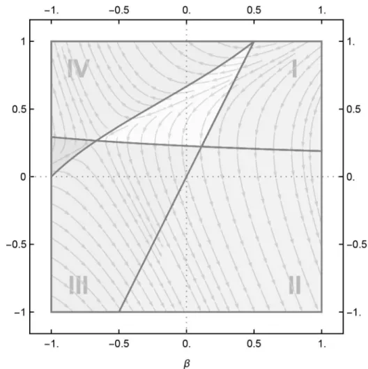
Fig 1illustrates how product rivalry and technology spillovers mediate optimal process R&D investments. The two subfigures display the optimal R&D investments inβ-σ space with the horizontal axis depicting knowledge spillovers (β), and the vertical axis, the degree of
Fig 1. Optimal R&D,x�, conditional onβ, σ and bγ. Arrows indicate a positive change in R&D investment for a
change in eitherβ or σ.
product substitution (σ). Subfigure (a) shows an example of low efficiency in R&D
invest-ments, assuming a high value forbγ (in the diagram, we assumed bγ = 50). The right panel in
Subfigure (b) depicts the case of highly efficient R&D investments withbγ = 4; note that this
value represents the infimum of the product of these two parameters. Below this value, the sec-ond-order condition, required to be negative for an optimal choice of R&D investment in the second stage of the game, will no longer be negative over the whole domain ofβ and σ. Hence, for some values ofσ and β (upper left and lower right corners of the β − σ space), the
second-order condition becomes positive, rendering R&D investments unbounded from above. The higherbγ, the closer the line, which spans the β-σ-space from left to right, to the vertical axis.
This observation will also be taken into account in the empirical part of the paper.
Furthermore, ifσ > 2β, the R&D levels of xiandxjare positively related: any change in firm
i’s R&D investments is associated with a corresponding change in firm j’s R&D investments. If
insteadσ < 2β, any change in firm i’s R&D spending leads to an opposite change in firm j’s
R&D investment.
The line connecting the points (β = −0.5, σ = 1) and (β = .5, σ = 1) inFig 1divides the β-σ-plane into two corresponding regions: the left region with substitutive R&D investment behav-ior and the right region with complementary investment behavbehav-ior. Whether complementary or substitutive R&D investment behavior leads to a higher or lower optimalx�
(β, σ) depends onβ and σ. The line between (β = −1, σ = 0) and (β = 0.5, σ = 1) and the line close to the vertical axis—the line which is mediated bybγ, as explained above—separate the plane into further
subregions. Due to the sensitivity of the model tobγ, we put our focus on the four regions, in
which R&D investment reactions of firms should be clearly observable in the data. To make sure that the limits of the regions do not get blurred in our empirical study, we reduce these four regions even further. The corners marked by dashed rectangles in Subfigure (b) ofFig 1 will form the basis of our analysis.
For further clarification of the two panels in this figure: The line running from (β = −1, σ = 0) to (β = .5, σ = 1) denotes all combinations of β and σ where @x�/@σ = 0. The second line
close to the horizontal axis, separating subregions I and IV from subregions II and III, sub-sumes allloci with @x�/@β = 0. The underlying stream plot in the two subfigures depicts the
direction of the highest slope in optimalx�
(β, σ) as mediated by σ and β. This leaves us with the following four major regions in theβ-σ space:
• Complementary R&D investment: 0 <dxi/dxj< 1 • Region I with @x�
/@σ < 0 ^ @x�
/@β < 0 • Region II with @x�/@σ < 0 ^ @x�/@β > 0
• Substitutive R&D investment:−1 < dxi/dxj< 0 • Region III with @x�
/@σ < 0 ^ @x�
/@β > 0 • Region IV with @x�/@σ > 0 ^ @x�/@β < 0
This model enlightens the rationale underlying process R&D decisions by firms. Such deci-sions not only impact firms’ own marginal costs but also affect rival companies’ decideci-sions by affecting their supply and demand curvesvia the contextual parameters β and σ, respectively.
More precisely, an increase in R&D investments by firmi entails several effects: (1) a shift of
firmi’s supply curve to the right by a magnitude of xi, as process innovation decreases mar-ginal costs, (2) a reallocation of market shares as in the standard Cournot model, and (3) a countervailing effect to effect (2) because technology spillovers also reduce the representative competitorj’s marginal costs by a magnitude of βxi, thus shifting its supply curve to the right.
Whether the representative competitorj eventually increases (resp. decreases) its R&D
investments in return, however, is unclear. This depends on the firm’s location in theβ-σ space. In Region I, both technology spillovers and product rivalry are high. If firmi increases
its R&D investments, the loss incurred by firmj due to the shift of its residual demand curve to
the left outweighs the loss incurred by technology spillovers when firmj increases its R&D
investments in return. Therefore, it is rational for firmj to also increase its level of R&D
investment.
Fundamentally, in Region I, diminished demand due to product rivalry dominates the enhanced supply that results from technology spillovers. This in turn renders process R&D less attractive for any cost-reducing innovation spread over a narrower scale of production. Therefore, firmi as well as the representative competitor j have a strong incentive to diminish
their research investments and the positive correlation between both firms’ R&D investments is due to the fact that each firm finds it beneficial to free ride on the other firm’s R&D.
Region II implies product complementarity with positive spillovers. An increase in process R&D by firmi reduces firm j’s marginal costs, shifting the supply curve downwards, and
increases demand for productj by shifting its demand curve upwards due to product
comple-mentarity. These mutually consistent demand and supply effects clearly act as an incentive for firmj to also increase its R&D effort as a result of the increased optimal quantity q�
j.
Condi-tional on a sufficiently high cost parameterγ, the convexity of the R&D cost function ensures the existence of an upper equilibrium. This increases the marginal return to firmj’s R&D,
incentivizing firmj to increase its R&D effort.
The positive correlation observed in Regions I and II must be distinguished from one another. In Region I, both firms reduce their R&D investments to benefit from their rivals’ efforts. Therefore, the collective level of R&D investments remains at a lower threshold, as depicted by the stream plots inFig 1. In Region II, however, both firms find it profitable to increase their R&D efforts. Hence, it is no surprise that the maximum level of R&D investment is found in Region II.
In Region III, where products are complements with large negative spillovers, an increase in process R&D by one company will, on the one hand, dissuade the other company to pro-duce more due to increased marginal costs, and, on the other hand, it will motivate the com-pany to produce more due to the increased demand that stems from product
complementarity. Because the upward shift in the supply curve dominates that in the demand curve, the company will decrease its output level. This in turn renders process R&D less attrac-tive and leads to a decreased level of process R&D by the rival company. In other words, there is substitution in process R&D.
Region IV also involves mutually consistent effects, but in the opposite direction. With neg-ative spillovers and product substitution, an increase in investment in process R&D by firmi
shifts the supply curve upwards the demand curve downwards, reducing the optimal quantity of the rival companyq�
j. This renders process R&D less profitable and acts as a disincentive to
invest in process R&D.
Our theoretical framework is compatible with but not identical to a series of models that link innovative activities and product market competition. This resembles the work of Aghion et al. [13], who argue that the relationship between competition and R&D activities is an inverted U-shaped relationship, implying that loose or fierce competition is detrimental to innovation. Instead, we argue that it is not only the level of competition alone that matters but also the level of spillovers.
Our theory says that the sign of the reaction functiondxi/dxjdepends on the location of firmi and its representative competitor j in the β-σ space. More precisely, we aim to estimate
the sign of the reaction functionf(xjt) for each of the four corners of theβ-σ space. In order not to run the risk that the effects ofβ and σ get blurred by the uncertainty of actual limits between regions, we decided to confine our empirical study as in our theoretical model even further. The two subfigures inFig 1illustrate that a low value ofbγ will reduce Region IV. Since neither b nor γ were observed in our data, the actual magnitude of bγ remains uncertain. Likewise, the
diagonal line between (β = −0.5, σ = 1) and (β = .5, σ = 1), separating Regions I and II from Regions III an IV, subsumes loci in which the sign of the derivatives with respect toβ and σ are close to zero. For these reasons, we look exclusively at the data that can be classified into the dashed rectangles in SubfigFig 1b.
Theory also warns about the stability of the reaction functions for Regions II and IV: with
sufficiently high research costs γ, the reaction functions are well-behaved and lead to a stable
equilibrium. This has been put forward by Henriques [14], who analyzes these conditions for the model by d’Aspremont Jacquemin [12]. In Region II, below a threshold value for research costγ, the reaction functions leads to an unstable equilibrium where full specialization by one firm occurs: only one company undertakes R&D activities, whereas the other chooses to with-draw from research activities. Moreover, for even lower levels ofγ, the second-order condi-tions may not be fulfilled for Region IV. Therefore,
dxi=dxj> 0 in Region I
dxi=dxj� 0 in Region II
dxi=dxj< 0 in Region III
dxi=dxj� 0 in Region IV
3 Empirical protocol
The empirical exercise is to estimate the R&D reaction functions between any two firmsi and j, as shown inEq (17), that is, to estimate the elasticity of R&D investment decisionsx made by
firmi with respect to the R&D investment of firm j:
xi ¼f ðxjÞ þ xi ð19Þ
To estimateEq (19), we need financial data on R&D decisions and other firm characteristics and data that would allow us to determine both the amount of potential spilloversβ and the level of product substitutionσ between any two firms i and j. Data on the world’s largest
corpo-rations allow us to address these issues.
3.1 Computing the empirical
β-σ space
The difficulty lies in measuring product substitutionσ and technological spillovers β between
any two firms to reveal the concealedβ-σ space. Reliance on the cosine index is pervasive in the literature since [15] to measure technological spillovers [16,17], Nesta Saviotti JIE 05. The rationale is that firms that develop competencies in similar technologies should benefit from each other’s advances in research, more so than companies that are active in entirely different fields. More recently, [1] rely on the cosine index to measure technology spilloversand
prod-uct market rivalry.
Because theory specifies that bothσ and β belong to the interval [−1; +1], reliance on the
coefficientr to compute proximity measures in the technology and product market space
which produces measures of product substitutionσ and of technological spillovers β that lie
between [−1; +1]. Observe that Pearson’s r is nothing else than the cosine index computed on mean-centered values.
Concerning technological spilloversβij, we proceed as follows. We use patent data to describe the firms’ portfolio of technological competencies and use the latter to measure pair-wise correlations in the technology portfolio for any dyad. Patent data come from the USPTO dataset provided by the National Bureau of Economic Research [18]. This dataset contains more than 3 million US patents issued since 1963. Using information on each company’s name and year of application, we selected the firms most active in patenting using the 2000 Edition of Who Owns Whom to control for firm consolidation. Importantly, the USPTO data-set assigns each patent to several international patent technology classes (IPC). The six-digit technology classes proved too numerous, so we adopted the three-digit level, corresponding to a technological space of 120 technologies.
Letpiktbe the number of patents applied for by firmi in technology class k during year t. Because the knowledge underlying a patent is durable for a longer time span, we assume that all patents have a life span of five years. Therefore, for a given technologyk, we define Tiktas the sum of patents over the past five years:Tikt ¼
P4
t¼0pik;t t. We can then describe the
techno-logical profile of companies by a vector of technotechno-logical competencies Tt, where generic
com-ponentTiktis the accumulated number of patents in a given technological field in a given year. Leaving the time subscript aside and writing ~T as the mean-centered vector of patents T,
tech-nological spilloversβijbetween the two vectors ~Tiwith ~Tjreads
bij¼ ~ T0 iT~j ffiffiffiffiffiffiffiffiffiffi ~ T0 iT~i q � ffiffiffiffiffiffiffiffiffiffi ~ T0 j ~ ~ Tj q ð20Þ
where the subscriptsi and j denote firms i and j, respectively. Two companies that are
develop-ing competencies in the same or similar vectors of technologies are supposedly more inclined to identify, assimilate and exploit each other’s R&D findings [19], thereby benefiting from the rival’s R&D and incorporating it into their own production function and decreasing the mar-ginal cost of production. The case of the nullity of the Pearson’sr implies full independence in
the firms’ technology portfolios, where neither positive technological externalities nor negative pecuniary externalities can occur. A negative correlation coefficient implies that areas of rela-tive specialisation of companyi represent areas of relative under-investment by company j.
Although in this case little gains from technological externalities can be expected, pecuniary externalities are likely to dominate.
Concerning product substitution, one would ideally use demand functions on particular pairs of products or even use the technological characteristics of products to measure the dis-tances between any pair [20]. In both cases, however, data are difficult to find, especially when they need to be combined with additional information on such areas as technology spillovers and company accounts. Instead of concentrating on all types of firms, we focus on multi-prod-uct firms and argue that prodmulti-prod-uct substitution, or the degree of market rivalry, can be measured using the vector of sales of companies across several market segments.
One could be tempted to adopt a similar reasoning as the one above for technological spill-overs. In this case, the idea is that firms competing on similar markets compete with one another. Suppose that multi-product companies can be described by a vector of sales Y, where generic componentYisprovides the amount (level) of sales by firmi for a given 4-digit sector segments. It is then straightforward to compute Pearson’s r between the two vectors ~Yiand
~
Yj. This calculation leads to slevij, the degree of market rivalry measured in levels:
slev ij ¼ ~ Y0 iY~j ffiffiffiffiffiffiffiffiffiffi ~ Y0 iY~i q � ffiffiffiffiffiffiffiffiffiffi ~ Y0 jY~j q ð21Þ
where subscriptsi and j denote firms i and j, respectively, and ~Y is the mean-centered vector of
sales across business segments.
However, there is an issue inEq (21)level as to whether the correlation coefficient of sales over several market segments really captures rivalry on the product market. Instead, one would use cross-product elasticities to properly grasp whether two goods are complements or substitutes. In order to approach the idea of cross-product elasticities, we transform the vector of sales Y in growth rates _y for all companies, and then compute the correlation coefficient
over the vector of growth rates as follows sgrij ¼ ~_y0 i~_yj ffiffiffiffiffiffiffiffi ~_yi~_yi q � ffiffiffiffiffiffiffiffiffi ~_y0 j~_yj q � 1 ð22Þ
Observe that the use of of growth rates implies that we multiply the Pearson’sr by −1. The
reason for this is that two firms enjoying a positive growth rate on the same business segment are likely to have complementary products, whereas two firms competing on the product mar-kets should cope with a negative correlation in the growth rates. Hence a positive correlation coefficient in the sales growth rates between any two firms implies product complementarity, a dimension which in our theoretical framework is depicted whenσ < 0.
In the empirical part, our preference goes toEq (22), although we will also conduct robust-ness checks usingEq (21)as a measure of rivalry on the product market side.
3.2 Control variables
Past research shows that R&D investment by firms is affected by factors other than the level of R&D investments of rival firms.
First, we include a proxy for the efficiency parameterγ inEq (3)and defineγias the patent productivity of R&D investments (P/X)i, whereP is the number of patents granted to firm i andX is the firm’s R&D investment. We lag this variable two years to avoid simultaneity in the
relationship. Second, [21] and [22] have stressed the interdependence of firm size and R&D investments. Because large firms have an advantage in spreading the cost of research over a larger span of output, R&D investments tend to increase monotonically with size. We there-fore include firm sizeK into the empirical model using the gross value of plant and equipment.
Third, strategic investment decisions also depend on financial constraints [23,24,25]. When returns on investments are subject to substantial uncertainty, as is the case with research activities, firms increase cash flow availability to secure in-house investment capacities as a response to the lack of external financial resources [26]. If markets were perfect, investment decisions could be financed by either internal means or external credit availability. In the pres-ence of imperfect markets, however, limited access to external financial resources will be com-pensated for by increases in cash availability provided by the firm itself. This makes it easier for the company to undertake investment decisions. We therefore include the so-called liquid-ity ratio (LR), defined as the cash flow availability normalized by current liabilities. Should
financial markets be imperfect, a positive association between R&D decisionsX and LR should
Because variables on firm size and financial constraints influence future decisions, we lag all control variables by one year. Moreover, we include a full vector of year dummies to account for the year-specific shocks common to all firms in the sample. Unobserved firm het-erogeneity is accounted for through the use of pre-sample mean panel data models.
3.3 Data sources
Compustat is the source of all firm-level accounting data. The gross value of property, plant and equipment proxies firm size (K); the liquidity ratio LR and the ratio between cash flow
availability and current liabilities are used to grasp financially constrained firms. Financial data, expressed originally in national currencies, have been converted into US dollars using the exchange rates provided by the Organisation for Economic Co-operation and Development (OECD). All financial data have been deflated in 2005 US dollars using the Implicit Price Deflator provided by the US Department of Commerce, Bureau of Economic Analysis.
Compiling the data from the patent and financial sources produced an unbalanced panel dataset of 308 companies observed between 1979 and 2005, yielding 5,461 firm-year observa-tions. These come from various industries that differ in their R&D intensity (X/Y). Of all
cor-porations, 199 belong to high-technology sectors, including Chemicals (63 firms), Electronic Equipment (54 firms), Photographic, Medical and Optical Goods (36 firms), and Industrial Machinery and Computer Equipment (46 companies), with an aggregate R&D intensity reach-ing 6%. There are 62 corporations in the medium-technology sectors, namely, in Transporta-tion Equipment (32 firms), Business Services (21 firms) and Other Sectors (9 firms), with an aggregate R&D intensity of between 3% and 5%. The low-technology sector comprises 47 firms (Furniture and Fixtures, 5 firms; Paper Products, Printing and Publishing, 12 firms; Petroleum and Refining, 10 firms; Rubber, Concrete and Miscellaneous Products, 8 firms; Metal Industries, 12 firms) (Table 1).
The Cournot-type model developed in Section (1) is based on two firms located in theβ-σ space. We must therefore compute allβij’s andσij’s between any pair of firms—a dyad—in the sample. Becauseβij=βjiandσij=σji,N × (N − 1)/2 β and σ measures are produced per year, depicting the nature of competition between any two companiesi and j.
Fig 2displays the number of dyads in the obtainedβ-σ space, expressed in deciles. It reveals that most companies tend to avoid direct product and R&D competition because they are located in the bottom-left corner of theβ-σ space. We also observe the absence of location in areas of strong technological and product rivalry, corroborating the idea that the largest corpo-rations develop firm-specific portfolios of business lines and technological competencies.
The figure also points at specific dyads. In Region I, we find dyads in two heavily competi-tive markets: Abbott Laboratories and Smithkline Beecham for the pharmaceutical preparation industry and the well-known rivalry between Ford and General Electric in the automobile industry. Fierce product market rivalry is also found in the case of Pfizer (pharmaceutical preparation) and Morton International (Miscellaneous chemical products), albeit with signifi-cantly different technology portfolios. The same applies to Litton Industries Inc. (Ship & boat building) and Ashland Inc. (Chemical and allied substances). In this Region (Region IV), firms may mainly suffer from the rival’s R&D efforts in that it increases the marginal cost of production due to pecuniary externalities.
At the bottom ofFig 2, we display three dyads that have market complementarity in com-mon. Although with a substantial level of technological overlap, market rivalry between Micro-soft and Apple appears lower as a result of the presence of Apple in the hardware industry, whereas Microsoft is committed to the Prepackaged Software industry. Complementarity in products appears in the case of Microsoft (Electronic computers) and IBM (Computer
Programming) with very similar technology portfolios. Because this dyad is located in Region II, the presence of positive spillovers is expected. This is the ideal location for dyads: each com-pany benefits from the R&D executed by the other comcom-pany, thus lowering its marginal cost. It also benefits from increased sales by the partner because of product complementarity. At the other extreme (Region III), we find dyads with product complementarity and dissimilar tech-nology portfolios such as Fiat (Motor Vehicles) with Litton Industries (Ship and boat build-ing). In this Region, the theory predicts that strategic partners suffer from each other’s R&D due to pecuniary knowledge externality.
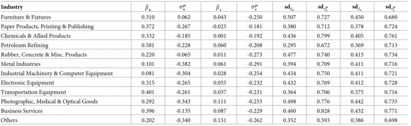
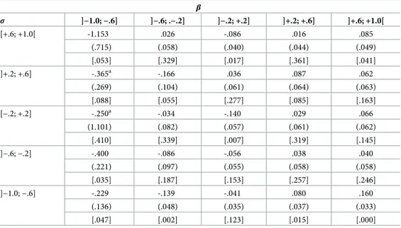
InTable 2, we display the mean values forβ and σ using the business lines provided by Compustat, which uses the standard industrial classification. We thereby distinguish dyads in which the two companies come from the same business line with respect to their main activity from those with different main business lines.
The potential for technology spillovers appears to be substantially higher for companies that share the same main business line. For all intra-industry dyads �bnis significantly positive, with an average value of .287 whereas the cross-industry dyads have an average value of �
bx¼ :046. No such pattern is found for product market rivalry, whereσgris negative and aver-ages at -.25 and -.24 for intra and cross-industry dyads. In fact, the Student t-test reveals that the difference in technological spillovers between intra and cross industry dyads is significant with a t-value of 190.00, whereas the difference in product market rivalry between intra and cross industry dyads is insignificant with a t-value of 1.42. The message ofTable 2is that: although two large, multi-product firms belonging to the same industry may be either rivals or deliver complementary products, the accumulation of technological competencies within an industry is less flexible. This is in line with Pavitt and Patel [27, p.156], who argue that contrary to the sphere of products, the sphere of technology “(. . .) is underpinned by quite rigid, one-to-one technology imperatives: if you want to design and make automobiles, you must know
Industry ] Firms ] Obs. Xa
Yb Kc i LR d ( X/Y)e ] Pg γh
Furniture & Fixtures 5 85 85.4 5,215 1,635 0.146 0.016 29.1 3.681
Paper Products, Printing & Publishing 12 212 229.7 9,507 8,924 0.210 0.024 65.1 10.200
Chemicals & Allied Products 63 1,120 676.0 9,625 7,476 0.748 0.070 101.8 16.570
Petroleum Refining 10 219 374.6 60,980 59,379 0.277 0.006 150.4 4.827
Rubber, Concrete & Misc. Products 8 130 155.9 5,840 3,748 0.243 0.027 38.4 5.313
Metal Industries 12 187 89.1 6,119 4,515 0.195 0.015 23.9 13.940
Industrial Machinery & Computer Equipment 46 850 540.1 9,384 4,930 0.545 0.058 163.3 9.704
Electronic Equipment 54 982 737.8 10,116 5,909 0.904 0.073 195.3 8.861
Transportation Equipment 32 575 1,506.0 37,635 21,608 0.223 0.040 146.4 17.470
Photographic, Medical & Optical Goods 36 614 266.2 4,432 2,552 0.523 0.060 93.0 9.226
Business Services 21 355 1,420.0 27,114 41,895 0.593 0.052 249.7 13.630
Others 9 132 1,231.0 36,280 25,868 0.256 0.034 299.3 13.680
All Sectors 308 5,461 688.2 15,598 12,277 0.567 0.044 141.5 11.820
a
X: R&D expenses, in millions of 2005 US$.
b
Y: Sales, in millions of 2005 US$.
c
K: Gross Property, Plant and Equipment, in millions of 2005 US$.
d
LR: Cash flow to current liabilities ratio.
e
X/Y: R&D intensity.
g
]P: Number of patents.
hγ: R&D Cost Parameter: γ = ]P/X.
Fig 2. Number of dyads in the empiricalβ-σ space, by deciles.
https://doi.org/10.1371/journal.pone.0232119.g002
Table 2. Average measures ofβ and σgrfor intra industry (n) and cross (x) industry dyads.
Industry b� n s� gr n b�x s� gr x sdbn sdsgrn sdbx sdsgrx
Furniture & Fixtures 0.310 0.062 0.043 -0.250 0.507 0.727 0.450 0.680
Paper Products, Printing & Publishing 0.372 -0.267 -0.025 -0.181 0.380 0.712 0.378 0.724
Chemicals & Allied Products 0.332 -0.185 0.001 -0.192 0.436 0.799 0.405 0.761
Petroleum Refining 0.581 -0.228 0.060 -0.208 0.295 0.672 0.369 0.713
Rubber, Concrete & Misc. Products 0.220 -0.065 0.011 -0.273 0.477 0.740 0.415 0.734
Metal Industries 0.101 -0.382 0.061 -0.291 0.394 0.709 0.411 0.716
Industrial Machinery & Computer Equipment 0.081 -0.304 0.028 -0.254 0.434 0.750 0.411 0.721
Electronic Equipment 0.315 -0.265 0.055 -0.232 0.432 0.769 0.412 0.728
Transportation Equipment 0.401 -0.261 0.037 -0.231 0.364 0.706 0.375 0.716
Photographic, Medical & Optical Goods 0.292 -0.343 0.111 -0.253 0.498 0.776 0.442 0.735
Business Services 0.396 -0.135 0.087 -0.229 0.460 0.828 0.432 0.771
Others 0.202 -0.340 0.131 -0.262 0.352 0.593 0.386 0.698
�
b and �sgrdenote arithmetic average of technological spillovers and product market rivalry, respectively. sd: Standard deviation
about mechanics; if you want to design and make aeroplanes, you must know about aeronau-tics (. . .)”
The above is corroborated when we look at the standard deviations of both technological spillovers and product market rivalry. In fact, the standard deviation is much lower for techno-logical spillovers than for product rivalry. This outcome is compatible with the presence of some form of technological determinism [27], whereas the scope for market location remains wide. In other words, product variety within an industry is fully compatible with technological homogeneity.
3.4 Econometric specifications
The empirical model estimates the reaction function of firmi in its R&D investment xit, condi-tional on firmj’s R&D investments xjt. First, we enter all variables in logs, estimating the elas-ticity ofxiwith respect toxj.
xit¼ a þ oxjtþ BCitþ xit ð23Þ
wheret = {1979, . . ., t, . . ., 2005}, lower cases indicate log transformed variables, ω is the
parameter of interest, and B is the vector of parameters of control variables Cit. This
econo-metric specification addresses three important issues, namely, firm unobserved heterogeneity, firmi’s decision-making process and the endogeneity of the RHS variable xjt.
First, unobserved variations in the characteristics of companies may influence firm R&D investments beyond and above the chief role of past R&D decisions, rival’s R&D investment, size and financial constraints. Such concealed dimensions may come from the firm’s research ties developed with private partners or/and with public research organizations, the organiza-tional culture of the company to be located at the forefront of the technological frontier, or, among other things, the CEO’s inclination to orient a research program towards ambitious and costly objectives. Ideally, one would include a firm-fixed effect to control for such unob-served attributes. However, within-transformations are known to produce inefficient estimates when samples are small and regressors are persistent, as is the case with R&D series. As an alternative estimator we use the pre-sample mean (PSM) estimator that replaces the fixed effect by the pre-sample mean of the dependent variable. [28] show that this estimator is consistent when the number of pre-sample periods is large for the dependent variable and has better finite sample properties than the fixed effect model. Therefore, we choose to include the pre-sample mean measure of the dependent variable, and constrain the pre-sample to include observa-tions after 1990 only, which yields the reaction function:
xit¼ a þ oxjtþ g�xipþ BCitþ xit ð24Þ
wheret = {1990, . . ., t, . . ., 2005}, and where xip¼ ð1=TPÞ
PTP
r¼0xi;1989 rrepresents the
pre-sam-ple mean,r = {0, . . ., r, . . ., TP} and TP is the number of pre-sample observations. Variable xip grasps persistent differences in R&D investments across firms and acts as a control for unob-served heterogeneity between firms.
Second, the duopoly model of the theoretical Section implies that each firm makes invest-ment decisions based on the optimal investinvest-ment of the rival company. Empirically, however, companies cope with an array of competitors so that the duopoly assumption is violated in most markets. In other words, the optimal R&D decision depends on the behavior of more than one rival only. Therefore, we assume that companies do not make inferences on their optimal R&D decisions based on each of their rivals. Similarly to [29], we assume that firms makeoblivious R&D choices, that is, decisions on R&D investments based on the R&D
decision of theaverage rival company. Specification (23) then becomes
xit ¼ a þ o�xjtþ g�xipþ BCitþ xit ð25Þ
Third, simultaneous decisions by companies imply that ifxiis determined byxj, the oppo-site relationship equally holds. This mutual dependence together with the specification inEq (24)calls for the use of additional moment restrictions that account for the correlation between endogenous variables �xjtwith the error termξit:
E xit; � xjt 1 � xst !! ¼ 0 ð26Þ
Note that part of the endogeneity should already be withdrawn when using �xj. When the
number of companiesn is high, individual decisions of firm i will influence �xjonly
margin-ally, i.e. by 1/(n − 1). We instrument �xjtby its own lagged values and computed variable �xst,
which measures the average level of investments in product segments at year t, as in the
fol-lowing: � xst¼ln P j6¼ixjst Ns 1 � �
withNsas the number of companies in business segments. Hence �xstis the (log of) average
R&D investment, the main business segment in which firmi is active, excluding firm i’s own
investment. Therefore, variable �xstis firm-specific.
Then, model25can be estimated using the well-known two step procedure, where the first step regresses the endogenous variable �xston its instruments and the second step includes
pre-dictions from the first step into the specification of interest, i.e. model (25). Four regressions are performed, one for each region in the empiricalβ-σ space. Based onFig 1, we assign dyads to the four regions as follows. Region I gathers dyads in which both technology spillovers and product substitution are positive, and the marginal effect of technology spillovers dominates the marginal effect of product substitution, i.e. 0 �βij� 1 ^ 0 �σij� 1 ^σij< 2βij. Region II concerns dyads in which product substitution is negative and the effect of technology spill-overs dominates the effect of product substitution:−1 � σij� 0 ^σ < 2β. Region III concerns dyads in which both technology spillovers and product substitution are negative−1 � βij� 0 ^−1 � σij� 0 ^σ > 2β. Region IV concerns dyads in which product substitution is positive and its marginal effect dominates the marginal effect of technology spillovers with 0 �σij� 1 ^ (β + 3)σ > β(σ2+ 2) + 2.
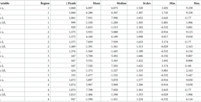
Table 3provides descriptive statistics for each region of the empiricalβ-σ space. It is note-worthy that product rivalry (σgr) divides dyads in two groups of similar size, where half com-pete on the product market (σgr> 0) and half sell complementary products (σgr< 0). By
exclusively focusing on competition on the product market (σ � 0), one actually screens out a
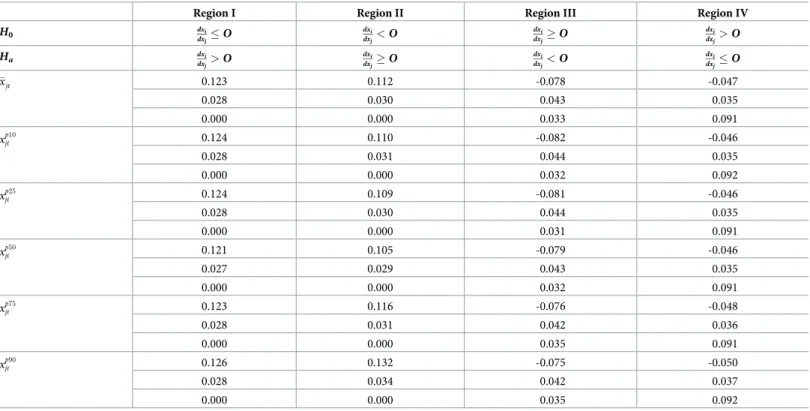
Our theory predicts thatω, the sign of the reaction function dxi/dxj, depends on the region of the dyads in theβ-σ space. Taking stock of the previous discussion, we expect the following:
H0: o � 0 ; Ha: o > 0 in Region I H0: o < 0 ; Ha: o � 0 in Region II H0: o � 0 ; Ha: o < 0 in Region III H0: o > 0 ; Ha: o � 0 in Region IV
4 Results
4.1 Main results
Table 4presents the results, where all sets of exclusion restrictions pass the Hansen test of validity of instruments. The results corroborate the theoretical predictions. In Regions I and II, the coefficient is both positive and significant, implying that a 1% increase in R&D investments by the representative rival company spurs the firm’s own research activities by .123% (Region I) and .112% (Region II), respectively. In Region III, a 1% increase in the representative rival
Table 3. Descriptive statistics by region.
Variable Region ] Dyads Mean Median St.dev. Min. Max.
lnxi 1 1,060 6.097 6.075 1.520 1.692 9.238 � xj 1 1,060 6.288 6.307 1.307 1.743 9.238 lnki 1 1,061 7.931 7.996 1.652 2.643 11.77 lnLRi 1 999 -1.330 -1.289 1.305 -5.881 1.906 γi 1 929 -1.635 -1.513 1.182 -6.532 3.001 lnxi 2 1,575 5.933 5.888 1.555 -0.916 9.115 � xj 2 1,575 6.160 6.189 1.098 0.017 9.030 lnki 2 1,575 7.839 7.939 1.623 3.174 11.77 lnLRi 2 1,489 -1.391 -1.361 1.313 -6.029 2.163 γi 2 1,376 -1.569 -1.445 1.189 -6.532 6.116 lnxi 3 447 5.700 5.492 1.606 -0.192 9.007 � xj 3 447 5.552 5.365 1.422 1.692 8.808 lnki 3 447 7.520 7.502 1.625 3.174 11.60 lnLRi 3 424 -1.373 -1.327 1.333 -5.881 2.163 γi 3 335 -1.677 -1.532 1.341 -6.532 5.447 lnxi 4 1,073 5.897 5.878 1.577 -0.916 9.030 � xj 4 1,074 5.967 5.968 1.206 -0.916 9.030 lnki 4 1,074 7.700 7.820 1.561 2.643 11.77 lnLRi 4 1,013 -1.406 -1.398 1.353 -6.029 1.906 γi 4 947 -1.590 -1.451 1.224 -6.532 6.116
See previous Table for the definition of variables. Region I: 2bij> sgr ij^ 0 < s gr ij < 1 Region II: 2bij> sgr ij ^ 1 < s gr ij < 0 Region III: 2bij< sgr ij ^ 1 < s gr ij < 0 Region IV: ðbijþ 3Þsgr ij > bijðs gr ij2 þ 2Þ þ 2 ^ 0 < s gr ij < 1 https://doi.org/10.1371/journal.pone.0232119.t003
firm R&D investments yields a.078% decrease in firmi R&D investments. In Region IV, the
estimated parameter ^o remains negative, although it is less significant and of a smaller magni-tude (−.047%). As mentioned earlier, the reaction function in Region IV may not reach the demand (slopeb) and R&D conditions (γ) required for stability. In other Regions of the β-σ
space, allω parameters are larger in magnitude and more efficient.
The parameter estimates that stem from the control variables conform to our expectations. First, firm size has a positive effect in all Regions. The liquidity ratio is significantly positively associated with levels of R&D investments in all Regions of theβ-σ space. The estimated short-run elasticities span from.36% to.40%. R&D investments embody a high level of uncertainty, which may hinder private external finance. As a response to the lack of external finance, firms may accumulate cash flow to secure the financing of future research activities. Moreover, low short-term liabilities can also be a sign of low financial constraints. In both cases, either high cash flow availability or low short-term liabilities increase the liquidity ratio thereby facilitating the financing of promising research projects.
Second,Eq (14)predicts thatγ, the R&D cost parameter, reduces optimal R&D x�
i. Our
results confirm that an increase in R&D costs will decrease R&D investments. This negative relationship may come from different channels. Increased R&D costs may be considered increased sunk costs, the profitability of which is highly uncertain. Increased R&D costs may also be considered increased fixed costs, increasing the minimum scale of post-innovation
Table 4. Firm-level reaction functions with contemporaneous R&D investments of the mean rival firm. IV GMM Regressions with Pre-Sample Mean �xip.
Region I (Model 1) Region II (Model 2) Region III (Model 3) Region IV (Model 4) � xjt 0.123 0.112 -0.078 -0.047 (0.028)��� (0.030)��� (0.043)�� (0.035)� kit 0.253 0.277 0.354 0.359 (0.039)��� (0.034)��� (0.055)��� (0.043)��� lnLRit 0.358 0.356 0.401 0.391 (0.028)��� (0.021)��� (0.046)��� (0.024)��� lnγit−1 -0.293 -0.308 -0.405 -0.297 (0.042)��� (0.034)��� (0.057)��� (0.037)��� � xip 0.430 0.430 0.322 0.371 (0.041)��� (0.033)��� (0.055)��� (0.038)��� Constant 1.206 0.997 1.988 1.862 (0.335)��� (0.315)��� (0.502)��� (0.367)��� Observations 650 992 276 691 R-squared 0.651 0.649 0.660 0.681 Hansen’s J 0.671 2.459 0.795 0.0337 Hansen c.p. 0.413 0.117 0.372 0.854 KP Wald F 6,678 5,058 4,274 6,419
Robust standard errors in parentheses.
���p<0.01, ��p<0.05, �p<0.1.
All regressions include a full vector of unreported year fixed effects. Endogenous regressorsxjtare instrumented using their past level and average sectoral R&D, net of the firm’s own R&D. In models 3 and 4,xjtis instrumented using average sectoral R&D to satisfy the exogeneity condition imposed by the Hansen’s J test.
SeeTable 3for definitions of Regions.
operations. In both cases, this may act as a counter-incentive for firms to implement new research projects, thereby decreasing overall R&D investments.
A further noteworthy outcome is the stability of all other parameter estimates that stem from the control variables. It suggests that the empirical model is correctly specified and rein-forces the finding that the sign of the reaction function depends on the location in theβ-σ space between any two companies, as suggested by the theoretical model.
4.2 Robustness checks
We perform robustness checks by addressing a number of issues related to the econometric specification. First, in order to account for the size of both firmsi and j, we assume that firms
decide on their R&D intensity, defined as the ratio of R&D investmentsX over firm size K.
Therefore, we amend specification (24) as follows:
lnðX=KÞit ¼ a þ olnðX=KÞjtþ glnðX=KÞipþ BCitþ xit ð27Þ
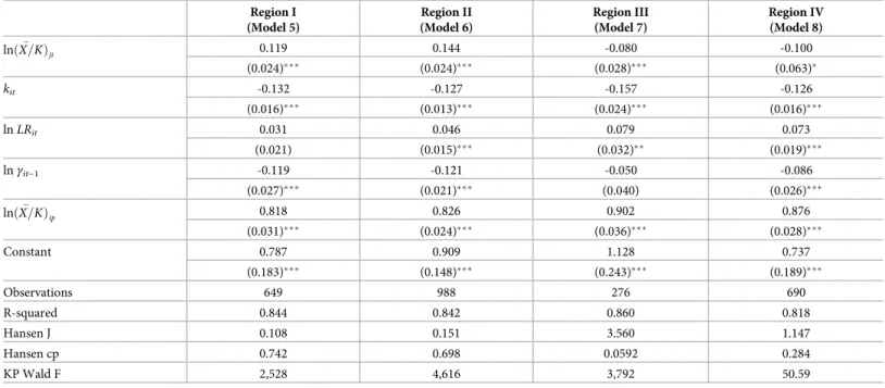
This amendment must be understood as a way of normalizing R&D investments. By con-trolling for the size of both firms, it is more in line with the Cournot model of Section (1), where symmetry in cost and production is assumed.Table 5displays the results. These remain unchanged in direction and magnitude with one notable exception. In Region IV with sub-stantial product substitution and negative technology spillovers, the parameter estimateω
Table 5. Firm-level reaction functions with contemporaneous R&D intensity of the mean rival firm. IV GMM Regressions with Pre-Sample MeanlnðX=KÞ� ip.
Region I (Model 5) Region II (Model 6) Region III (Model 7) Region IV (Model 8) � lnðX=KÞjt 0.119 0.144 -0.080 -0.100 (0.024)��� (0.024)��� (0.028)��� (0.063)� kit -0.132 -0.127 -0.157 -0.126 (0.016)��� (0.013)��� (0.024)��� (0.016)��� lnLRit 0.031 0.046 0.079 0.073 (0.021) (0.015)��� (0.032)�� (0.019)��� lnγit−1 -0.119 -0.121 -0.050 -0.086 (0.027)��� (0.021)��� (0.040) (0.026)��� � lnðX=KÞip 0.818 0.826 0.902 0.876 (0.031)��� (0.024)��� (0.036)��� (0.028)��� Constant 0.787 0.909 1.128 0.737 (0.183)��� (0.148)��� (0.243)��� (0.189)��� Observations 649 988 276 690 R-squared 0.844 0.842 0.860 0.818 Hansen J 0.108 0.151 3.560 1.147 Hansen cp 0.742 0.698 0.0592 0.284 KP Wald F 2,528 4,616 3,792 50.59
Robust standard errors in parentheses.
���p<0.01, ��p<0.05, �p<0.1.
All regressions include a full vector of unreported year fixed effects. Endogenous regressors ln(X/K)jtare instrumented using their past level and average sectoral R&D, net of the firm’s own R&D. In models 7 and 8, ln(X/K)jtis instrumented using average sectoral R&D to satisfy the exogeneity condition imposed by the Hansen’s J test. SeeTable 3for definitions of Regions.
doubles in size, implying that a 1% increase in R&D investments by the representative rival company decreases the firm’s own research intensity by.10%.
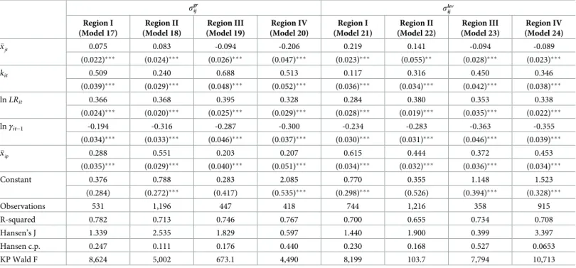
The previous results are based on the use ofσgrin order to detect product market rivalry between dyads. Although we strongly believe that this measure grasps important aspects of product complementarity and substitution between two firms’ array of products, an alternative way of measuring product market rivalry is simply to assess the similarity of their market posi-tioning usingσlev.Table 6displays the results for both the level of R&D investment (specifica-tion25, left panel) and R&D intensity (specification27, right panel). Note that the Pearson’sr
correlation coefficient betweenσgrandσlev(not reported in the Table) amounts to−.023, only. This implies that the firms detected as product complements or substitutes differ from one sample to the other.
Although being larger in magnitude, the estimated elasticities comply to our hypotheses, corroborating the idea that the reaction function in strategic investments may be either
Table 6. Firm-level reaction functions with contemporaneous R&D decisions of the mean rival firm. Usingσ to measure product rivalry. IV GMM Regressions with Pre-Sample Mean �xipandlnðX=KÞ� ip, respectively.
R&D Investments R&D Intensity
Region I (Model 9) Region II (Model 10) Region III (Model 11) Region IV (Model 12) Region I (Model 13) Region II (Model 14) Region III (Model 15) Region IV (Model 16) � xjt 0.393 0.212 -0.129 -0.030 (0.050)��� (0.046)��� (0.075)�� (0.021)� kit 0.243 0.231 0.301 0.232 -0.101 -0.095 -0.114 -0.102 (0.033)��� (0.026)��� (0.062)��� (0.025)��� (0.010)��� (0.009)��� (0.015)��� (0.010)��� lnLRit 0.274 0.300 0.229 0.300 0.047 0.051 0.032 0.038 (0.022)��� (0.016)��� (0.046)��� (0.016)��� (0.011)��� (0.011)��� (0.015)�� (0.011)��� lnγit−1 -0.250 -0.246 -0.184 -0.244 -0.116 -0.120 -0.090 -0.125 (0.034)��� (0.027)��� (0.049)��� (0.024)��� (0.016)��� (0.016)��� (0.021)��� (0.016)��� � xip 0.502 0.543 0.532 0.550 (0.035)��� (0.027)��� (0.065)��� (0.025)��� � lnðX=KÞjt 0.193 0.138 -0.038 -0.058 (0.021)��� (0.022)��� (0.018)��� (0.042)� � lnðX=KÞip 0.782 0.837 0.933 0.908 (0.023)��� (0.019)��� (0.021)��� (0.021)��� Constant -0.935 -0.012 1.445 1.800 0.542 0.486 0.626 0.483 (0.459)�� (0.433) (0.566)�� (0.264)��� (0.183)��� (0.187)��� (0.200)��� (0.199)�� Observations 888 1,471 265 1,719 1,506 1,804 585 1,708 R-squared 0.699 0.700 0.732 0.706 0.840 0.828 0.859 0.812 Hansen’s J 1.363 0.414 0.373 0.207 0.00214 1.483 0.524 1.566 Hansen c.p. 0.243 0.520 0.541 0.649 0.963 0.223 0.469 0.211 KP Wald F 188.6 302.4 45.14 20,017 7,614 8,805 3,966 119.7
Robust standard errors in parentheses.
���p<0.01, ��p<0.05, �p<0.1.
All regressions include a full vector of unreported year fixed effects. Endogenous regressorsxjtare instrumented using their past level and average sectoral R&D, net of the firm’s own R&D. In models 11 and 12,xjtis instrumented using average sectoral R&D to satisfy the exogeneity condition imposed by the Hansen’s J test. Endogenous regressors ln(X/K)jtare instrumented using their past level and average sectoral R&D, net of the firm’s own R&D. In models 15 and 16, ln(X/K)jtis instrumented using average sectoral R&D to satisfy the exogeneity condition imposed by the Hansen’s J test.
SeeTable 3for definitions of Regions.