Flow control using optical sensors

(1)

HAL Id: tel-01150428

https://tel.archives-ouvertes.fr/tel-01150428

Submitted on 11 May 2015

Flow control using optical sensors

Nicolas Gautier

To cite this version:

Nicolas Gautier. Flow control using optical sensors. Mechanics of the fluids [physics.class-ph].

Uni-versité Pierre et Marie Curie - Paris VI, 2014. English. �NNT : 2014PA066640�. �tel-01150428�

(2)

Ecole doctorale: Sciences m´

ecaniques, acoustique, ´

electronique & robotique

(UPMC)

ESPCI, Laboratoire PMMH

Flow control using optical

sensors

(Contrˆ

ole d’´

ecoulement par capteurs optiques)

Nicolas Gautier

Th`ese de doctorat de Physique

Dirig´

ee par Jean-Luc Aider

Jury

Dr. Fran¸cois Lusseyran (Rapporteur)

LIMSI

Dr. Denis Sipp

(Rapporteur)

ONERA

Dr. Philippe Guibert

(Examinateur)

UPMC

Dr. Azeddine Kourta

(Examinateur)

PRISME

Dr. Bernd Noack

(Examinateur)

PPRIME

(3)

0.1 Abstract

Flow control using optical sensors is experimentally investigated. Real-time computation of flow velocity fields is implemented. This novel approach featuring a camera for acquisition and a graphic processor unit (GPU) for processing is presented and detailed. Its validity with regards to speed and precision is investigated. A comprehensive guide to software and hardware optimization is given. We demonstrate that online computation of velocity fields is not only achievable but offers advantages over traditional particle image velocimetry (PIV) setups. It shows great promise not only for flow control but for parametric studies and prototyping also.

A hydrodynamic channel is used in all experiments, featuring a backward facing step for sep-arated flow control. Jets are used to provide actuation. A comprehensive parametric study is effected to determine the effects of upstream jet injection. It is shown upstream injection can be very effective at reducing recirculation, corroborating results from the literature. Both open and closed loop control methods are investigated using this setup. Basic con-trol is introduced to ascertain the effectiveness of this optical setup. The recirculation region created in the backward-facing step flow is computed in the vertical symmetry plane and the horizontal plane. We show that the size of this region can be successfully manipulated through set-point adaptive control and gradient based methods.

A physically driven control approach is introduced. Previous works have shown success-ful reduction recirculation reduction can be achieved by periodic actuation at the natural Kelvin-Helmholtz frequency of the shear layer. A method based on vortex detection is intro-duced to determine this frequency, which is used in a closed loop to ensure the flow is always adequately actuated. Thus showing how recirculation reduction can be achieved through simple and elegant means using optical sensors.

Next a feed-forward approach based on ARMAX models is implemented. It was successfully used in simulations to prevent amplification of upstream disturbances by the backward-facing step shear layer. We show how such an approach can be successful in an experimental set-ting.

Higher Reynolds number flows exhibit non-linear behavior which can be difficult to model in a satisfactory manner thus a new approach was attempted dubbed machine learning control and based on genetic programming. A number of random control laws are implemented and rated according to a given cost function. The laws that perform best are bred, mutated or copied to yield a second generation. The process carries on iteratively until cost is minimized. This approach can give surprising insights into effective control laws.

(4)

classique.

Un canal hydrodynamique est utilisé pour toutes les expériences. Celui-ci comporte une marche descendante pour le contrôle d’ écoulements décollés. Les actionneurs sont des jets. Dans le cas de la marche descendante une étude paramétrique approfondie est faite pour qualifier les effets d’une injection en amont des jets, celle-ci étant traditionnellement ef-fectuée à l’arrête de la marche.

Plusieurs méthodes de contrôle sont étudiées. Un algorithme de contrôle basique de type PID est mis en place pour démontrer la viabilité du contrôle d’écoulement en boucle fermée par capteurs optiques. La zone de recirculation située derrière la marche est calculée en temps réel dans un plan vertical et horizontal. La taille de cette région est manipulée avec succès.

Une approche basée sur des observations de la dynamique de l’écoulement est présentée. Des résultats précédents dans la littérature montrent que la recirculation peut être réduite avec succès en agissant sur l’écoulement à la fréquence naturelle de lâchés tourbillonnaires liés à l’instabilité de Kelvin-Helmholtz de la couche cisaillée crée par la marche. Une éthode basée de détection de vortex est introduite pour calculer cette fréquence, qui est ensuite utilisée dans une boucle de contrôle qui assure que l’écoulement est toujours pulsé à la bonne fréquence. Ainsi en utilisant des capteurs optiques la recirculation est réduite de fa¸con simple.

Ensuite nous implémentons un contrôle de type feed-forward dont l’efficacité a préalablement été démontrée en simulation. Cette approche vise à prévenir l’amplification de perturba-tions amont par la couche cisaillée. Nous montrons comment une telle méthode peut être implémentée avec succès dans un contexte expérimental.

Enfin, nous implémentons également une approche radicalement différente basée sur un algo-rithme génétique. Des lois de contrôle aléatoires sont testées et évaluées. Les meilleurs sont répliquées, mutées et croisées. Ce processus se poursuit itérativement jusqu’à ce que le coût soit minimisé. Bien que lente à converger cette approche donne des résultats encourageants `

(5)

0.3 Preface

This thesis deals with flow control using optical sensors. part I presents the basic concepts and methods. Part II contains the results. All but the first chapter of part II feature papers. They are adjusted to comply with the format of this manuscript, however their contents have not been altered. The introduction and core experimental setup, described in part I are common to all studies, thus the reader should not be amiss by skipping to the results sections in subsequent chapters.

1. T. Cambonie, N. Gautier, and J-L Aider. 2013

Experimental study of counter-rotating vortex pair trajectories induced by a round jet in cross-flow at low velocity ratios,

Experiments in Fluids, post-print available on the arXiv 2. N. Gautier, and J-L Aider. 2014

Real-time planar flow velocity measurements using an optical flow algorithm imple-mented on GPU,

To be published in Journal of Visualization, post-print available on the arXiv 3. N. Gautier, and J-L Aider. 2013

Control of the flow behind a backward-facing step by visual feedback, Royal Society Proceedings A, post-print available on the arXiv 4. N. Gautier, and J-L Aider. 2014

Effects of pulsed actuation upstream a backward-facing step, CRAS, post-print available on the arXiv

5. N. Gautier, and J-L Aider. 2014

Experimental frequency lock control of the flow behind the backwards facing step, Under consideration for publication in Experiments in fluids, pre-print available on the arXiv,

6. N. Gautier, and J-L Aider. 2014

Feed-forward control of the backward-facing step flow,

Under consideration for publication in Journal of Fluid Mechanics, pre-print available on the arXiv

7. N. Gautier, J-L Aider, T. Duriez, B.R. Noack, M. Segond, M. Abel. 2014

Closed-loop control of a wall-bounded separation experiment using machine learning, Under consideration for publication in Journal of Fluid Mechanics, pre-print available on the arXiv

(6)

8.3.4 Uncontrolled flow . . . 135 8.3.5 Actuation . . . 135 8.4 ARMAX model . . . 136 8.4.1 Introduction . . . 136 8.4.2 Model Computation . . . 138 8.4.3 Linearity . . . 141 8.5 Results . . . 141 8.5.1 Control law . . . 141 8.5.2 Control results . . . 144 8.6 Conclusion . . . 145 8.7 Acknowledgments . . . 145

(9)

9 Closed-loop control of a wall-bounded separation experiment using ma-chine learning 150 9.1 Abstract . . . 151 9.2 Introduction . . . 151 9.3 Experimental Setup . . . 152 9.3.1 Water tunnel . . . 152

9.3.2 Backward-Facing Step geometry . . . 153

9.3.3 Sensor: 2D real-time velocity fields computations . . . 153

9.3.4 Actuator . . . 154

9.4 Machine Learning Control . . . 154

9.4.1 Population generation . . . 157

9.4.2 Evaluation . . . 157

9.4.3 Breeding of subsequent generations and stop criteria . . . 158

9.5 Results . . . 159

9.5.1 Convergence of machine learning control . . . 159

9.5.2 Analysis of the best control law obtained through genetic programming 160 9.5.3 Comparison to periodic forcing . . . 162

9.5.4 Robustness . . . 164

9.7 Acknowledgements . . . 165

9.8 Appendix . . . 169

9.8.1 Control laws and expression trees. . . 169

9.8.2 Genetic programming operations on expression trees. . . 169

10 Conclusions & Perspectives 171 10.1 Conclusion . . . 171

10.2 Perspectives and considerations . . . 172

10.2.1 Application to drag measurements . . . 172

10.2.2 Real-time stereoscopic velocity field computations . . . 172

10.2.3 Real-time computation of three-dimensional velocity fields . . . 172

A Experimental study of counter-rotating vortex pair trajectories induced by a round jet in cross-flow at low velocity ratios 174 A.1 Abstract . . . 174

A.2 Introduction . . . 174

A.3 Experimental setup . . . 176

A.4 Trajectory computation . . . 179

A.5 Definition and relevance of the momentum ratio rm. . . 182

A.6 Influence of experimental parameters on CVP trajectories . . . 184

(10)

(11)

Part I

(12)

Chapter 1

Introduction

The research effected during this thesis sits at the interface of several disciplines: fluid mechanics, control theory and computer vision.

1.1 Flow control

In addition to being of significant academic interest fluids play a large role in a plethora of industrial applications. A few examples: automobile, aircraft and ship drag, mixing in combustion chambers, and cooling in nuclear power plants (figure 1.1).

(13)

While a wealth of information can be learned through observation, some seek to go be-yond observation, to control. Active flow control is at the interface of fluid mechanics and control theory. Through flow control we could increase vehicle efficiency, reducing our carbon emissions and improving operating costs, mitigating future rises in oil and gas prices. Un-fortunately fluids are not so easily commanded, they can be tricky and capricious. Exerting any kind of influence is a difficult task.

The governing equations (Navier-Stokes equations, described in appendix B) for most com-mon fluids, namely water and air, have been known for the past two-hundred years. Despite this a formal mathematical solutions eludes mathematicians and physicists alike. Thus nu-merical simulations and experiments are used to investigate fluids. Solving these equations numerically is possible but time consuming. Furthermore it is only possible for small vol-umes and simple geometries. In fact if there are no groundbreaking advances in computing technology completely solving the Navier-Stokes equations for practical flows will remain unattainable. Experimental work, while cumbersome, unyielding and error prone, remains essential to scientific process.

Flow control is a vast discipline. There are two categories for any type of control: passive and active control. Passive means of flow control, where no energy is supplied to the system are common. Automobiles for example are optimized to reduce aerodynamic drag as illustrated on figure 1.2 illustrates this.

(a) High drag shape (b) Lower drag shape (twice the aerodynamic ef-ficiency)

Figure 1.2

More sophisticated passive control methods involve adding flow control devices to the vehicles. For example in Godart and Stanislas (2005), Godart et al. (2005a,b) passive vortex generators are used to control a decelerating boundary layer. In Aider et al. (2010) active

(14)

form. Despite its advantages, passive control has limitations, most notably, once the system is tuned to specific working conditions everything is fixed. Therefore if operating conditions change too much control might become ineffective, or in some cases make things worse. To enable further improvement active control is considered.

(a) Passive blowing to lower drag induced by the wheels

(b) Active vortex generators on the concept Citro¨en C-Airlounge

Figure 1.3

Control is called active when energy is supplied to the system. Active flow control can be further sub-categorized into open and closed loop control. Wing flaps and rudders on airplanes and boats are a form of active open loop flow control. Energy is supplied to the flaps allowing them to move, thereby modifying airflow around them. Open loop means the control action is not based on any observations of the flow. Open-loop control is common in flow control. The first open-loop active control demonstration for a full sized airplane was performed by Wygnanski (2004). In Protas and Wesfreid (2002a) a cylinder is rotated, for certain configurations this drives the mean flow towards a lower drag state. In Joseph et al. (2013) micro jets were used to increase pressure recovery on the rear of an Ahmed body. In Shaqarin et al. (2013) open-loop control is used to limit separation of a turbulent boundary layer after a sharp variation in wall geometry (a ramp).

(15)

1.2 Closed-loop control

The distinction between active and open loop control is fundamental as open-loop control methods cannot adapt to unexpected changes in operating conditions. Closed loop control requires a sensor component. Information is obtained by one or several sensors, which is used to determine optimal control action. Furthermore since the system is monitored, changes in the environment or the system itself can be accounted for ensuring an element of stability and robustness. The great benefits of closed loop control are balanced by its complexity: poorly implemented control can saturate actuators, possibly damaging the system or causing additional unsteadiness. Control theory deals with every manner of closed-loop approaches. The first formal analysis of the field was conducted by James Clerk Maxwell Maxwell (1868) on governors. Figure 1.4 shows an example of closed loop control in the human body.

Figure 1.4: Sketch of closed loop control in biology

Since then the field has become a scientific domain of its own. Applying this knowledge to flow control has yielded many different approaches. Here we will briefly detail the main types of approaches, highlighting the advantages and disadvantages of each as well as cases of successful implementation. This, by no means an exhaustive list, is meant to give the reader context and a better understanding of the different flow control approaches featured in this work.

1.2.1 Adaptive control

Adaptive control does not require a model for the system, which is its biggest asset. At each instant system state is ascertained through measurements. The goal of adaptive control is to

(16)

with other non-linear designs to control the span-wise recirculation length downstream a step in Henning and King (2007). This approach has since been expanded upon and used for to alter the lift configuration of a full sized wing (Kerstens et al. (2011)), which could lead to different lift-off and takeoff procedures for airplanes, potentially increasing the throughput of a given airport.

Slope-seeking algorithms are used to bring a measured variable of a system such as drag to an extremum. No modeling is required. Moreover the technique is quite robust. Any system featuring a extrema is susceptible to this type of control. This approach does places several constraints on actuation. In order for this approach to work a low frequency component must be added to actuation. A detailed explanation of this method can be found in Ariyur and Krstic (2004). This is a very general method. In Beaudoin et al. (2006) extremum-seeking is used to pilot a cylinder placed at the separation edge of a bluff body. The same approach is used for an Ahmed body in Beaudoin et al. (2008). Control is able to quickly minimize drag behind the body, resulting in a positive energy balance. In Pastoor et al. (2008) the shear layer behind a bluff body is controlled using a combination of jets together with pressures gauges. A wide array of control methods are featured in this study including extremum and slope-seeking which are used to maximize pressure recovery behind the body, leading to reduced drag. In general it is more difficult to implement than PID controllers.

It should be noted that model-independent controllers while very robust take some time to adapt to changing flow condition making them potentially slower than model based con-trollers.

1.2.2 Model based control

Another approach consists in modeling the flows as non-linear systems of infinite order (derived from the Navier-Stokes equations). Attempts have been made to design a controller based on the full-order Navier-Stokes equation. In Bewley (2001) optimal control is used on low Reynolds number DNS simulations. Protas and Wesfreid (2002b) use a vorticity equation derived from the Navier-Stokes formula for optimal control. While no reduction is made this kind of approach requires full knowledge of the flow (restricting it to 2D flows for now) and is computationally costly making it impractical for practical applications. However such an approach can be used to determine the full potential of an actuator or given control method.

On the opposite side of the spectrum lie phenomenological models based on observations of the physics of the flow. This approach cannot be made systematic and is not always applicable. However when it is relevant it can yield very simple models for the dominant dynamics of the flow leading to fast and efficient control. For example the wake behind a cylinder at low Reynolds number behaves like a non-linear oscillator (Provansal et al. (1987)) and can be modeled in a very simple fashion (Protas and Wesfreid (2002a), Thiria et al. (2004)). In Pastoor et al. (2008) several control methods are applied to reducing bluff body drag. The study culminates on the development of a very simple physics based model linking the output of a single pressure sensor to edge actuation. The control displays the same drag reduction as extremum-seeking while being 50 times faster at producing the reduction.

In practice however most attempts at model-based flow control feature a reduction step in which a low-order model is created, either directly from the Navier-Stokes equations or

(17)

empirical data from simulations and/or experiments. Such a step is crucial in model design. If the flow exhibits linear behavior a number of approaches are possible, J.Kim and Bewley (2007). When it comes to controlling linear systems, control theory literature is very rich. Linear models for flow control have been the subject of intensive study. In Becker et al. (2005) simple linear black-box models are used to describe the behavior of recirculation behind an experimental step, leading to the set point control of recirculation length. Most of the work on linear models for flow control is done in numerical simulations. Linear models can be derived from Galerkin projection of the linearized Navier-Stokes Equation, Rowley et al. (2004). These models are of very high order making computation of the control output too long for real-time control, thus they must first be reduced. Studies show using balanced POD modes yield efficient reduced-order models, Moore (1981), Rowley (2005). In Belson et al. (2013) linear reduced order models are used to determine optimal sensor/actuator placement for the control of a Blasius boundary layer. In Barbagallo et al. (2009) linear quadratic gaussian control is used with reduced order models to stabilize the unstable flow created by an open cavity. In Bagheri et al. (2009) a framework for input-output analysis leading to linear reduced order models is presented.

Linear models enable the use of powerful tools from control theory such as discrete time optimal and model predictive control, therefore it is enviable to seek such models for flow systems. Unfortunately most flows of interest are intrinsically non-linear. Making a linear model approach difficult. Furthermore few have applied these methods to experimental flows. Non-linear modeling is much harder, and thus less common. However examples exist, low-dimensional modeling has been used to effect successful sliding mode control of a bluff body wake, Luchtenburg (2010). Such control is a special case of variable structure control, a form of non-linear discontinuous control. The feedback control law is not a continuous function of time, it switches from one smooth condition to another potentially very quickly. The advantages of this particular method are robustness with regards to model uncertainty and convergence in finite time. However it is likely to quickly wear out actuators (due to fast switching) imposing heavy engineering constraints.

1.2.3 Machine learning

Finally, a radically different approach can be applied handle non-linearities. Genetic pro-gramming has been used in other disciplines for some time, when applied to flow control it makes novel approaches possible. It can be used to look for optimal, possibly non-linear control laws. Randomly generated control laws are evaluated with respect to a user defined cost function, from then on the process is completely hands-off. It allows for great freedom in terms of possible controls laws. New counter-intuitive laws can more easily be found by-passing any user bias. This approach is new to flow control. Theoretical and experimental work can be found in Duriez et al. (2014) and chapter 9.

(18)

Figure 1.5: An approach to flow control

1.3 The special case of separated flows and the

back-ward facing step geometry

The work presented in this manuscript focuses on the control of separated flows. These are ubiquitous in nature and industrial processes. Figure 1.6 illustrates examples of such flows. In automobile applications, separated flows cause most of the drag experienced by the vehicle. Recirculation on airfoils causes drag and sometimes severe loss of lift. Ma-nipulating separation leads to pressure drag reduction, lift enhancement, stall delay, heat transfer improvement, dynamic load reduction and attenuation of excess noise and vibra-tion. Additionally the performance of fans, turbines, compressors, pumps, and diffusers may be increased by delaying the onset of separation. In the case of separated flows open-loop control has been widely investigated: cavity control, Backward-facing step control, Ramp control, Ahmed Body. Because of it similarity to a moving ground vehicle, the Ahmed body, in all its declinations has been intensively studied, Vino et al. (2005), Fares (2006), Pujals et al. (2010), Joseph et al. (2012, 2013).

(19)

(a) Flow around a wing (b) Flow inside a combustion chamber

(c) Flow around a car

Figure 1.6

Several geometries can be used to study separated flows, such as the backward facing step, the inclined and rounded ramps. Figure 1.7 illustrates these common geometries. Red and dotted lines indicate typical recirculation locations and shape. Note that for the backwards facing step geometry separation is imposed by the edge, while for configurations feature a mobile separation point.

(20)

(a) Step (b) Ramp

(c) Rounded ramp (Duriez et al. (2008))

Figure 1.7

The backward facing step has the advantage of being the simplest possible geometry. Flow separation is imposed at the step edge and therefore perfectly localized in space as shown in figure 1.8. The main feature of the backward facing step flow is the recirculation region, which appears as a result of separation. This flow has been extensively studied both numerically and experimentally (Armaly et al. (1983), Hung et al. (1997), Beaudoin et al. (2004), Aider et al. (2007)). Historically recirculation length has been used to characterize the flow as a whole. In flow control experiments recirculation reduction is almost always the control objective (Chun and Sung (1996), Becker et al. (2005)). However it is interesting to note there is no clear relationship between recirculation size and drag, as shown in chapter 3.

Figure 1.8: Sketch of a backward facing step

1.4 Optical sensors

Optical sensors can be used to effect flow measurements. There are many types of optical sensors, the most common is the human eye. Unfortunately one cannot download data from

(21)

them (yet). Therefore we rely on the now ubiquitous video camera. At its most fundamental level a video camera is a photon counting device, doing so many times per second (as opposed to a regular camera) ultimately yielding a series of images. An entire scientific field known as computer vision is dedicated to acquiring, processing, analyzing, and understanding images, usually all this is done in real-time.

Cameras have been used to quantitatively investigate fluid dynamics for over three decades. A common technique consists in seeding the flow with neutrally buoyant particles which act as tracers allowing the experimentalist to compute the flow velocity field. This method is invaluable as it yields rich quantitative information on the state of the flow, in addition velocity fields are essential to the numerical fluids mechanics community as it allows for validation of numerical experiments. However such a process can be burdensome. A typical experiment yields tens of thousands of images which have to be transfered from the camera buffer or the acquisition computer to a computing cluster to a personal workstation for analysis and post-processing. This process can be slow and inconvenient taking up to several days.

Particle Image Velocimetry (PIV) is widely used to compute 2D velocity fields (Westerweel (1993), Melling (1997), Wil (2007), U. G¨ulan (2012)). In PIV the image is discretized into sub-windows containing an average of five to ten particles. Their motion is estimated using cross correlation between two successive images. High particle concentration is required for optimal resolution. Adrian (2005) gives a thorough review of PIV methods. Other techniques exist to compute flow velocity fields. Particle Tracking Velocimetry (PTV) is based on the tracking of single particles between two successive images (L¨uthi et al. (2005)). Particle concentration is typically an order of magnitude lower for PTV. Optical flow has been used in computer vision to compute image intensity displacement in robotic applications. It has successfully been used on images intended for PIV processing (Faure et al. (2010)). Figure 1.9 illustrates the fundamental difference between PIV and PTV.

(22)

Figure 1.10: Experimental setup featuring wall sensors

Most closed-loop flow control experiments feature wall sensors (pressure, shear rate, see figure 1.10). An essential part of any control loop is the sensor, traditionally wall sensors are used in flow control experiments. Figure 1.10 shows a set-up featuring an array of pressure sensors designed to compute the extent of the recirculation bubble.

Pressure and friction sensors are the most common, they output local data at high fre-quencies. Their main disadvantage is that they give an incomplete snapshot of the flow. Furthermore the parietal nature of the information can make it difficult to access informa-tion far from the wall. Computing the flow state using incomplete informainforma-tion is a subject of ongoing research usually involving sophisticated techniques such as Kalman filters. In some cases a few well placed sensors give sufficient information for successful control (Pastoor et al. (2008)). However determining the most effective placement for these sensors requires time consuming parametric studies.

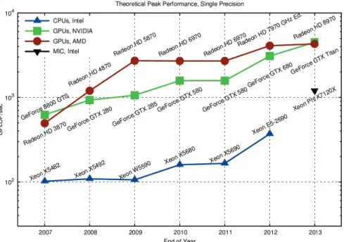
Recent increases in computing power allow us to consider real-time, i.e. high frequency low latency computation of velocity fields. Essentially binding image acquisition, processing and post-processing into a single streamlined process. This turns every pixel of the camera into a sensor yielding a wealth of information and direct unfettered access to the flow state. Because of rising user demand for graphic intensive applications personal computers now feature both a central processor unit (CPU) and a graphic processor unit (GPU). In terms of raw computing power the GPU far outclasses the CPU as shown in figure 1.11. This is because GPU’s feature a massively parallel architecture, using thousands of processing cores whereas modern CPU’s typically feature only 4. The difference between CPU and GPU processing is succinctly and colorfully explained in Sav (2010).

Recently GPU programming has become increasingly accessible thanks to efforts made by manufacturers. Programming languages such as OpenCL and CUDA now provide extensions to common languages such as C++ and Fortran. However not all programs benefit from a GPU implementation in the same way. In some cases performance can worsen. In chapter

(23)

Figure 1.11: CPU vs GPU processing power trend, note the logarithmic scale

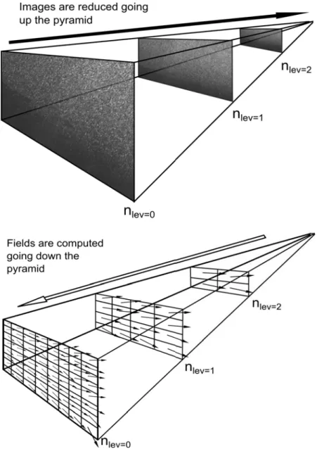
4 we will show how computer code developed at ONERA and subsequently improved over the course of this thesis is parallelized to leverage the awesome power of the GPU enabling real-time computation of flow velocity fields.

1.5 Actuation

There are many ways to act on a flow. Cattafesta and Sheplak (2011) gives a thorough review of the different possible actuators. Figure 1.12a shows a possible actuator classifi-cation. In dense fluids like water, jet actuation is widely used (Rathnasingham and Breuer (1990), Jacobsen and Reynolds (1998)) however other less conventional means of control have been investigated. Most notably moving the wall itself (Breuer et al. (1989), Endo et al. (2000), Du et al. (2002), Iwamoto et al. (2005), Koberg (2007)). Deployable flaps have shown promise as vortex generators (Choi et al. (1994)). Underwater speakers are another potential option.

When the fluid is lighter such as air, actuators are more plentiful. A lot of research has gone into making viable plasma actuators (T. Duriez (2014), Thomas et al. (2009)). Electrodes

(24)

force is perfectly tangential to the flow allowing for better near wall actuation. The main disadvantage of plasma actuators is that they cannot yet accelerate the fluid past 10 m.s−1 which is to slow for practical applications to external aerodynamics of air and ground vehi-cles.

Speakers placed in the flow are a popular method for acting on light fluids Chun and Sung (1996), Henning and King (2007), they are simple, cheap and easy to control. Mechanical flaps are used for control on airplanes and ships as well as flow control experiments (Lai et al. (2002)). Blowing/suction using jets is also widely used (Yoshioka et al. (2001), Uruba et al. (2007)). Figure 1.12b shows different types of actuators applied to a backward facing step configuration, from Garrido (2014). One should note actuators such as jets or solid vortex generators can be placed upstream the step edge and remain effective as will be shown in chapter 6.

The work presented in this manuscript features wall jets as actuators. The reason for this is twofold: wall jets are relatively easy to implement and remain the simplest way to effect actuation in a dense fluid such as water. Furthermore this work was part of a broader research effort by the instability, control and turbulence team at PMMH. Past researchers have focused on studying the effect of jets on the flow Beaudoin (2004), Duriez (2009), Cambonie (2012). The study of jets in cross-flow is a vast area of fluid mechanics, indeed their behavior is far from simple. Furthermore they occur in a number of natural and industrial processes such as air injection in gas turbines, thrust vector control for high speed vehicles and exhaust plumes for power plants. Making their study relevant to industry. For more information on transverse jets see Karagozian (2010), Margarson (1993).

The beginning of this work was devoted to studying round jets in cross-flow using a novel volumetric velocimetry technique. Three cameras (with set angles) are used to capture a laser illuminated flow volume. Identifying the same particle in all three images allows for the determination of particle position in 3D space. Once this has been done for all image triplets standard tracking techniques are used in pairs of triplets to determine particle velocity, finally interpolation is used to yield a regular 3D velocity grid for the observed volume. This allows for the computation of experimental three-dimensional instantaneous fields. The focus was primarily on jet trajectories. In an effort to further qualify actuation the objective was to determine a scaling law allowing us to predict the position of a jet beforehand. The ultimate goal being better actuators which could better affect the flow, leading to better control. This work culminated in a global scaling law for low velocity ratio round jets, published results are shown in appendix A (Cambonie et al. (2013)). Further exploitation of these and other 3D fields featuring jets with round or different geometries can be found in Cambonie and Aider (2014).

1.6 Control of the recirculation past a backward facing

step

Open-loop control of the backward facing step flow has been investigated for a wide range of operating conditions, actuators and sensors. Table 1.1 summarizes the results of several past studies with regards to open-loop performance. The focus was on recirculation length reduction. The most effective actuators are the flapping foil placed inside the shear layer Lai

(25)

(a) Summary of different actuators applied to the backward facing step flow, from Cattafesta and Sheplak (2011)

(26)

Reh Sth Xr/Xr,0 Device Location Method Chun and Sung (1996) 13 − 33000 0.27 65 % Open-loop: Loudspeaker

Step edge Experimental

Lai et al. (2002) 12700 0.18 30 % Open-loop: Flapping foil Immerged shear layer Experimental Yoshioka et al. (2001)

1800 − 5500 0.19 69% Open-loop: Slots Step edge Experimental

Chun et al. (2004)

33000 0.2 89% Open-loop:

Wake generator

Step back Experimental Uruba

et al.

(2007)

35000 0 31 % Open-loop:

Blowing/Suction

Step bottom Experimental

Garrido (2014) 30000 0.25 20 % Open-loop : Plasma DBD Upstream step Experimental Henning and King (2007) 0-25000 - 65 % Closed-loop: Loudspeakers

Step edge Experimental

Wengle

et al.

(2001)

3000 0.21/0.48 67 % Open-loop:

Loudspeakers

Step edge Numerical (DNS/LES) Neumann and Wen-gle (2003) 3000 0 87 % Open-loop: Fences Upstream Numerical (DNS/LES)

Table 1.1: Results from past studies for recirculation manipulation

et al. (2002), and continuous suction/blowing at the step bottom Uruba et al. (2007). In the flapping foil case the best placement is where vortex shedding would begin in the uncontrolled shear layer. While considerable reduction is accomplished, introducing a flap inside the flow poses engineering constraints and might be impractical in a more realistic setting. Continuous suction/blowing at the bottom of the step induces significant reduction in Uruba et al. (2007). The only downside might be actuation cost, as constant blowing and/or suction requires more energy than pulsed actuation. It is worthy of mention however that in simulations by Dahan and Morgans (2012) at Reh ≈ 10000 pulsed suction/blowing

at the step bottom has very little effect (5 % reduction).

1.7 Thesis organization

The first part of this thesis is organized as follow. Chapter 2 presents the experimental setup, chapter 3 general thoughts on the qualification of separated flows, chapter 4 the GPU algorithm used to effect real-time velocity computations, Chapter 6 the effects of upstream

(27)

actuation, Chapter 5 our first attempt at flow control by visual feedback, Chapter 7 physically driven separated flow control, Chapter 8 feed-forward control of the backward facing step flow, chapter 9 presents the results obtained using a genetic algorithm.

(28)

Bibliography

Particle Image Velocimetry - A Practical Guide. Springer, 2007. video : Adam and jamie paint the mona lisa in 80 milliseconds, 2010.

R. J Adrian. Twenty years of particle image velocimetry. Exp. Fluids, 39(2):159–169, August 2005.

J-L. Aider, A. Danet, and M. Lesieur. Large-eddy simulation applied to study the influence of upstream conditions on the time-dependant and averaged characteristics of a backward-facing step flow. Journal of Turbulence, 8, 2007.

Jean-Luc Aider, Jean-Fran¸cois Beaudoin, and Jos´e Eduardo Wesfreid. Drag and lift reduction of a 3d bluff-body using active vortex generators. Exp. Fluids, 48(5):771–789, 2010. Kartik B. Ariyur and Miroslav Krstic. Slope seeking: a generalization of extremum seeking.

International journal of adaptive control and signal processing, 18:1–22, 2004.

B. F. Armaly, F. Durst, J. C. F. Pereira, and B Schonung. Experimental and theoretical investigation of backward-facing step flow. J. Fluid Mech, 127:473–496, 1983.

S. Bagheri, D.S. Henningson, J. Hoepffner, and P.J. Schmid. Input-output analysis and control design applied to a linear model of spatially developing flows. Applied Mechanics Reviews, 62, 2009.

A. Barbagallo, D. Sipp, and P.J. Schmid. Closed-loop control of an open cavity flow using reduced-order models. J. Fluid Mech, 641:1–50, 2009.

J-F. Beaudoin. Active control and modal structures in transitional shear flows. PhD thesis, PSA-ESPCI, 2004.

J-F. Beaudoin, O. Cadot, J-L. Aider, and J.E. Wesfreid. Three-dimensional stationary flow over a backwards-facing step. European Journal of Mechanics, 38:147–155, 2004.

J.-F. Beaudoin, O. Cadot, J.-L. Aider, and J. E. Wesfreid. Drag reduction of a bluff body using adaptive control methods. Physics. Fluids, 18:1, 2006.

J-F. Beaudoin, O. Cadot, J-E. Wesfreid, and J-L. Aider. Feedback control using extremum seeking method for drag reduction of a 3d bluff body. IUTAM Symposium on Flow Control and MEMS, 7:365–372, 2008.

(29)

R. Becker, M. Garwon, C. Gutknecht, G. Barwolff, and R. King. Robust control of separated shear flows in simulation and experiment. Journal of Process Control, 15:691–700, 2005. B.A. Belson, O. Semeraro, C.W. Rowley, and D.S. Hennginson. Feedback control of

insta-bilities in the two-dimensional blasius boundary layer: The role of sensors and actuators. Physics of fluids, 25, 2013.

T.R. Bewley. Flow control: new challenges for a new renaissance. Prog. Aerospace Sci, 37: 21–58, 2001.

K.S. Breuer, J.H. Haritonidis, and M.T. Landahl. The control of transient disturbances in a flat plate boundary layer through active wall motion. Phys. Fluids, 1(574), 1989. T. Cambonie. Study of low velocity ratio jet in cross-flows by volumetric velocimetry. PhD

thesis, ESPCI, 2012.

T. Cambonie and J-L. Aider. Transition scenario of the round jet in crossflow topology at low velocity ratios. available on the arXiv, 2014.

T. Cambonie, N. Gautier, and J-L. Aider. Experimental study of counter-rotating vortex pair trajectories induced by a round jet in cross-flow at as a function of rehvelocity ratios.

Exp. Fluids, 54(3):1–13, 2013.

L. Cattafesta and M. Sheplak. Actuators for active flow control. Annu. Rev. Fluid Mech, 43:72–247, 2011.

H. Choi, P. Moin, and J. Kim. Active turbulence control for drag reduction in wall-bounded flows. J. Fluid Mech, 262(75), 1994.

K. B. Chun and H. J Sung. Control of turbulent separated flow over a backward-facing step by local forcing. Exp. Fluids, 21:417–426, 1996.

S. Chun, Y. Zheng Liu, and H. Sung. Wall pressure fluctuations of a turbulent separated and reattaching flow affected by an unsteady wake. Exp. Fluids, 37:531–546, 2004. J. Dahan and A. Morgans. Feedback control for form-drag reduction on a bluff body with a

blunt trailing edge. J. Fluid Mech, 704:360–387, 2012.

Y. Du, V. Symeonidis, and G.E. Karniadakis. Drag reduction in wall-bounded turbulence via a transverse travelling wave. J. Fluid Mech, 457(1), 2002.

T. Duriez. Control of separated flows using vortex generators. PhD thesis, ESPCI, 2009. T. Duriez, J-L. Aider, and J.E. Wesfreid. Non-linear modulation of a boundary layer induced

(30)

T. Endo, N. Kasagi, and Y. Suzuki. Feedback control of wall turbulence with wall deforma-tion. Int. J. heat Fluid Fl, 21(568), 2000.

E. Fares. Unsteady flow simulation of the ahmed reference body using a lattice boltzmann approach. Comput. Fluids, 35:940–950, 2006.

T. Faure, C. Douay, S. Mochki, F. Lusseyrand, and G. Quenot. Stereoscopic piv using optical flow: investigation of a recirculating cavity flow. 8th International ERCOFTAC Symposium on Engineering Turbulence Modeling and Measurements, 3:905–910, 2010. Patricia Sujar Garrido. Active control of the turbulent flow downstream of a backward facing

step with dielectric barrier discharge plasma actuators. PhD thesis, Poitiers University, 2014.

M. Garwon, L.H. Darmadi, F. Urzynicok, G. B¨arwolff, and R. King. Adaptative control of separated flows. Proc. of the 2003 European Control Conference, Cambridge UK, 2003. G. Godart and M. Stanislas. Control of a deccelerating boundary layer. part 1: Optimisation

of passive vortex generators. Aero. Sc. Technol, 10(3):181–191, 2005.

G. Godart, J.M. Foucault, and M. Stanislas. Control of a deccelerating boundary layer. part 2: Optimisation of passive vortex generators. Aero. Sc. Technol, 10(5):394–400, 2005a. G. Godart, J.M. Foucault, and M. Stanislas. Control of a deccelerating boundary layer. part

2: Optimisation of passive vortex generators. Aero. Sc. Technol, 10(6):455–464, 2005b. L. Henning and R. King. Robust multivariable closed-loop control of a turbulent

backward-facing step flow. Journal of Aircraft, 44, 2007.

L. Hung, M. Parviz, and K. John. Direct numerical simulation of turbulent flow over a backward-facing step. J. Fluid Mech, 330:349–374, 1997.

K. Iwamoto, K. Fukagata, N. Kasagi, and Y. Suzuki. Friction drag reduction achievable by near wall turbulence manipulation at high reynolds numbers. Phys. Fluids, 17, 2005. S. Jacobsen and W.C. Reynolds. Active control of streamwise vortices and streaks in

bound-ary layers. J. Fluid Mech, 360(179), 1998.

J.Kim and T.R. Bewley. A linear systems approach to flow control. Annu. Rev. Fluid Mech, 39:383–417, 2007.

P. Joseph, X. Amandolese, and J. L Aider. Drag reduction on the 25 degrees slant angle ahmed reference body using pulsed jets. Exp. Fluids, 52(5):1169–1185, May 2012. P. Joseph, X. Amandolese, C. Edouard, and J.-L Aider. Flow control using mems pulsed

micro-jets on the ahmed body. Exp. Fluids, 54(1):1–12, 2013.

Ann Karagozian. Transverse jets and their control. Progress in Energy and Combustion Science, 36(5):531–553, OCT 2010.

W. Kerstens, J. Pleiffer, D. Williams, R. King, and T. Colonius. Closed-loop control of lift for longitudinal gust suppression at low reynolds numbers. AIAA Journal, 49(8), 2011.

(31)

H. Koberg. Turbulence control for drag reduction with active wall deformation. PhD thesis, Imperial College, 2007.

S.J.C. Lai, J. Yue, and M.F.Platzer. Control of a backward-facing step flow using a flapping foil. Exp. Fluids, 32:44–54, 2002.

B. L¨uthi, A. Tsinober, and W. Kinzelbach. Lagrangian measurement of vorticity dynamics in turbulent flow. J. Fluid Mech, (528):87–118, 2005.

Dirk Martin Luchtenburg. Low-dimensional modelling and control of separated shear flows. PhD thesis, Berlin Institute of Technology, 2010.

R.J. Margarson. Fifty years of jet in cross flow research. AGARD, pages 1–141, 1993. J. Maxwell. On governors. Proc. Royal Society, (100), 1868.

A. Melling. Tracer particles and seeding for particle image velocimetry. Measurement Science and Technology, (8), 1997.

B. Moore. Principal component analysis in linear systems: Controllability, observability, and model reduction. IEEE Trans. Autom. Control, 26(1):17–32, 1981.

J. Neumann and H. Wengle. Dns and les of passively controlled turbulent backward-facing step flow. Flow, Turbulence and Combustion, 71:297–310, 2003.

Mark Pastoor, Lars Henning, Bernd R. Noack, Rudibert King, and Gilead Tadmor. Feedback shear layer control for bluff body drag reduction. J. Fluid Mech, 608:161–196, 2008. B.S.V. Patnaik and G.W. Wei. Controlling wake turbulence. Phys. Rev. Lett, 88, 2002. B. Protas and J. Wesfreid. Drag force in the open-loop control of the cylinder wake in the

laminar regime. Phys. Fluids, 14(808), 2002a.

B. Protas and J. E. Wesfreid. Drag force in the open-loop control of the cylinder wake in the laminar regime. Physics. Fluids, 14:810, 2002b.

M. Provansal, C. Mathis, and L. Boyer. Benard-von k´arm´an instability: transient and forced regimes. J. Fluid Mech, 182:1–22, 1987.

G. Pujals, S. Depardon, and C. Cossu. Drag reduction of a 3d bluff-body using coherent streamwise streaks. Exp. Fluids, 49:1085–1094, 2010.

R. Rathnasingham and K.S. Breuer. Active control of turbulent boundary layers. J. Fluid Mech, 495(209), 1990.

(32)

T. Shaqarin, C. Braud, S. Coudert, and M. Stanislas. Open and closed-loop experiments to identify the separated flow dynamics of a thick turbulent boundary layer. Exp. Fluids, 54: 1432–1114, 2013.

J. Wesfreid G. Artana T. Duriez, J-L. Aider. Control of a backward-facing step flow through vortex pairing and phase locking. arXiv, 2014.

B. Thiria, S. Goujon-Durand, and E. Wesfreid. Fluid structure interaction as a factor of drag modification. J. Fluids Struc, 2004.

F. Thomas, T. Corke, M. Iqbal, A. Kozlov, and D. Schatzman. Optimization of dielectric barrier discharge plasma actuators for active aerodynamic flow control. AIAA Journal, 47 (9), 2009.

M. Holzner A.Liberzon A. Tsinober W. Kinzelbach U. G¨ulan, B. L¨uthi. Experimental study of aortic flow in the ascending aorta via particle tracking velocimetry. Exp. Fluids, 53(5): 1469–1485, 2012.

V. Uruba, P. Jonas, and O. Mazur. Control of a channel-flow behind a backward-facing step by suction/blowing. Heat and Fluid Flow, 28:665–672, 2007.

G. Vino, S. Watkins, P. Mousley, J. Watmuff, and S. Prasad. Flow structures in the near wake of the ahmed mode. J. Fluids Struct, 2005.

H. Wengle, A. Huppertz, G. B¨arwolff, and G. Janke. The manipulated transitional backward-facing step flow: an experimental and direct numerical simulation investigation. European Journal of Mechanics - B/Fluids, 20:25–46, 2001.

J. Westerweel. Digital particle image velocimetry: theory and application. PhD thesis, TU Delft, 1993.

I. Wygnanski. The variables affecting the control of separation by periodic excitation. AIAA Paper, pages 2004–2505, 2004.

S. Yoshioka, S. Obi, and S. Masuda. Organized vortex motion in periodically perturbed turbulent separated flow over a backward-facing step. Int.l Journal of Heat and Fluid Flow, 22:301–307, 2001.

(33)

Chapter 2

Experimental setup

The experimental work presented in this manuscript was effected in a hydrodynamic channel using the following setup.

2.1 Hydrodynamic channel

In this hydrodynamic channel the flow is driven by gravity. A single pump is used for water motion. Water is pumped from a bottom tank to a top tank in a continuous closed loop (see figure 2.1c). The pump is fully submerged and uses ambient water for cooling purposes, this induces a steady rise in temperature. For short experiments this is not a problem as water temperature is monitored and does not vary over the course of the acquisition, longer experiments (up to a week) must be done when water temperature has reached a plateau and viscosity stays constant. The flow in the test section is stabilized by divergent and convergent sections separated by honeycombs (see figure 2.1c). This is done to make the flow laminar and avoid disturbances in the flow downstream. Furthermore any large scale structures created upstream are nullified after passing through the honeycomb mesh. Figure 2.1c shows a sketch of the channel, figure 2.1a shows a rendering of the channel and figure 2.1b

The quality of the main stream can be quantified in terms of flow uniformity and turbulence intensity. The standard deviation σ is computed for the highest free stream velocity of our experimental setup. We obtain σ = 0.059 cm.s−1 _{which corresponds to turbulence levels of}

σ

U∞ = 0.0023. The channel is fully instrumented: water level, temperature and flow rate

are constantly monitored. This is done so that experiments can be more easily reproduced. Furthermore it is convenient to monitor water level so that longer running, unsupervised experiments can be stopped should any problems arise. Free stream velocity U∞varies from

(34)

(a) Computer rendering of the channel

(b) Rendering of the test section with a flat plate, can be switched for the backward facing step configuration.

(35)

(c) Sketch of the hydrodynamic channel

Figure 2.1

2.2 Leading edge and boundary layer thickness

A custom made plate with a specific leading-edge profile (NACA0019, shown in figure 2.1b and 2.6e) is used to start the boundary layer. Figure 2.2 compares experimental and the-oretical velocity profiles at the step edge, illustrating the laminar nature of the boundary layer. Results deviate from the typical Blasius profile near the wall because velocity field computation involves a correlation window, thus near wall results are limited by the size of the window which in turn is limited by displayed particle density. Mean shape factor

(36)

(d) Reh= 250 (e) Reh= 900

(f) Reh= 1350 (g) Reh= 3380

Figure 2.2: Experimental velocity profiles at the step edge (blue) and Blasius velocity profiles (green) for select Reynolds numbers (additional Reynolds numbers can be found in appendix D)

Figure 2.3 shows the evolution of boundary layer thickness at the step edge with Reynolds number, as is expected δ ∝ √1

Reh.

Figure 2.3: Boundary layer thickness scaled by step size as a function of Reynolds number

2.3 The backward facing step

Briefly introduced in the introduction the backward facing step is a benchmark for the study of separated flows. The backward facing step geometry and the main geometric parameters are shown in figure 2.4a. Step height is h = 1.5 cm. Channel height is H = 7 cm for a channel width w = 15 cm. The vertical expansion ratio is Ay = _h+HH = 0.82 and the

span-wise aspect ratio is Az= _h+Hw = 1.76. The injection slot is located d/h = 2 upstream of the

(37)

(a) Sketch of the backward facing step geometry and definition of the main parameters

(b) Vertical and horizontal observation planes

Figure 2.4

2.4 Jet injection

Jet injection is initiated in a pressurized tank. A water cooler will suffice for such an ap-plication. However they are not very durable and will break (sometimes explosively) after some time (from a couple of days to several weeks depending on usage). A resilient tank was devised and built using Plexiglas, it has not broken (yet). This allows for suction and injection as low pressures will cause the tank to fill up while high pressures while cause the tank to empty. A water level indicator is placed inside the tank, allowing for refilling. This

(38)

Figure 2.5: Jet supply circuit

Jet exit is handled by the system described in figure 2.6. The water goes through the plenum described in figures 2.6a and 2.6b. It is filled with glass beads sandwiched between two grids. This was designed to homogenize the flow prior to its entry in the injection chamber which is past the top grid. After the injection chamber the flow goes through cover plates of varying geometries. Examples of such cover plates are shown in figures 2.6c for a round jet and 2.6d for a vortex generator configuration. Cover plates are 11 cm across, and 3 cm wide. This system is advantageous as it is highly modular, virtually any exit geometry can be achieved by changing cover plates. Cover plate height can also be modified to change jet exit velocity profile. Figure 2.6e shows the jet injection system combined to a flat plate geometry for boundary layer control.

(a) Jet injection system (b) Jet injection side view

(c) Round jet cover plate (d) Vortex generator cover plate

(39)

(e) Jet injection system combined to a flat plate

Figure 2.6

Figure 2.7 shows different jet exit configurations. The round jet displayed in figure 2.7f was used (with varying diameters and injection lengths) in the study of jet trajectories described in appendix A. The studies featured in part II make use of the configuration shown in figures 2.7h and 2.7i.

(f) Round configuration

(40)

(h) Slot configuration

(i) Inclined slot configuration

(j) Vortex generator configuration

Figure 2.7

This automation was developed for the work presented in chapter 9 and has proved particularly effective at facilitating parametric studies. Figure 2.8 shows the relationship between pressure and flowrate for a given tank and tank height above the ground. It should be noted tank design has changed a lot through the course of this thesis. Therefore figure 2.8 should be taken as a qualitative example and is not correct for all studies featured in part II. For each study jet flowrate was determined independently. Flowrate is used instead of jet exit velocity as slots of different sections are used to provide actuation.

Figure 2.8: Flowrate as a function of pressure in the jet supply tank, for a standard slot configuration flow velocity can vary from−0.15 cm.s−1 _{to 20 cm.s}−1

(41)

2.5 Real-time velocity computation

The specifics of how real-time velocity field computations were achieved are detailed in chap-ter 4, they involve the implementation of a GPU algorithm for computing displacements akin to PIV. This method was developed as a means to an end for closed-loop control, however it also holds significant intrinsic worth as a tool for flow investigation. Arguably the method does not yield fields of significantly greater quality than traditional, much slower techniques. However it holds tremendous potential for fast prototyping and tuning in addition to con-siderably improving user comfort.

It brings ease and speed of use to the user as a single workstation can be used for acquisition, processing and post-processing. This aspect should not be underestimated as transferring data from computer to computer can be quite tedious. Furthermore computations are ef-fected much faster. With the right setup thousands of velocity fields can be computed per second. Results are instantaneous, flow data streams seamlessly to the user allowing for flow state assessment and operating parameters adjustment.

This leads to quicker, more relevant and more pleasant (a benefit which should not be under-estimated) experimental campaigns. More widespread implementation of real-time methods in a field still relying heavily on experimental results would greatly accelerate scientific dis-covery.

With respect to control, this method can be used to quickly evaluate control algorithms and determine which parameters and measurement make a given control approach viable. Real-time velocimetry can then be replaced by more specialized, targeted sensors for practical applications. The method greatly accelerated the studies presented in chapters 6, 8, and 9 in which control could have been accomplished using parietal sensors.

All the velocity data featured in this work save the study described in chapter 4 was obtained using this method.

(42)

Part II

(43)

Chapter 3

Characterization of the

backward facing step flow

Recirculation occurs behind a step at all Reynolds numbers. It is an important feature of many separated flows. It is the most significant feature of the backward-facing step flow and thus is often used to characterize the flow state (Armaly et al. (1983), Chun and Sung (1996)) and as a control objective in flow control experiments (Henning and King (2007)). Its characteristics (such as length) are relatively easy to measure. This chapter will review different ways in which recirculation can be qualified.

3.1 1D: recirculation length

There are many ways of defining recirculation length Xr. The most common is described in

equation (3.1) for isotropic incompressible flows, v = v(x, y, z, t) corresponds to longitudinal velocity, y is perpendicular to the bottom wall of the step, η (m2.s−1) is fluid viscosity.

Xr= x(τw= 0), τw= η ∂v ∂y _y=0 (3.1) Other definitions result in the same qualitative behavior, as demonstrated by the data featured in figure 3.1a. It shows recirculation length evolution as a function of Rehbased on

step height. It also shows the evolution of different length relevant to the confined backward facing step flow. Figure 3.1b shows recirculation length evolution for different data sets and varying expansion ratios (ratio of step height to channel height). These figures illustrate the robust nature of recirculation length evolution, whatever the definition, whatever the

(44)

(a) Evolution of recirculation length (x1), from Armaly et al. (1983)

(b) Evolution of recirculation length, different definitions, E is the expansion ratio (ratio of step height to channel height), from Thomas Duriez (2009)

(c) Evolution of recirculation length

(45)

p0_rms downstream the step exhibits a clear maximum slightly upstream of the reattachment point. This has been corroborated by Kiya and Sasaki (1983), Cherry et al. (1984), Lee and Sung (2001), Hudy et al. (2003). Microphone arrays in the bottom downstream wall can be used (in air) to easily detect p0rms making control of the recirculation length possible. This

technique was successfully used by Henning and King (2007).

3.2 2D: recirculation area

The definition for Xrdescribed in equation (3.1) is ill suited to 2D velocity fields. In addition

to being computationally costly it only uses the most noisy part of the available data, which is velocity vectors near the wall. A straightforward manner of qualifying recirculation in a 2D field is described in equation (3.2).

Ar(t) =

Z

A

H(−v(t))(x, y) dA (3.2)

(a) Instantaneous longitudinal velocity field at Reh= 2700

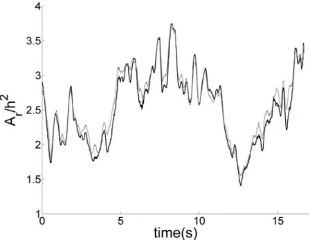
(b) Corresponding Ar(t) Reh= 2700 Figure 3.2

(46)

straightforward and intuitive, however it should be noted it is one amongst many ways of defining recirculation area. Figure 3.4 shows an example of Ar(t) for Reh= 1800, the time

series exhibits large fluctuations (δAr≈ 3.5h2).

Figure 3.3: Ar(t) for Reh = 1800, red triangle correspond to characteristic states of the

backward facing step flow

Figure 3.4 illustrates the evolution of time averaged recirculation area < Ar>twith Reh.

In red are select Reynolds numbers, that will be used throughout this chapter to illustrate specific states of the flow. Complementary fields for other Reynolds numbers can be found in appendix C. The qualitative agreement across multiple data sets highlights the universal nature of recirculation behavior for the backward facing step.

Figure 3.4: Time averaged, normalzied Arfunction of Reh

Unfortunately the time averaging operator does not commute with (3.2), this mean the time averaged recirculation area < Ar >t does not correspond to the recirculation area of

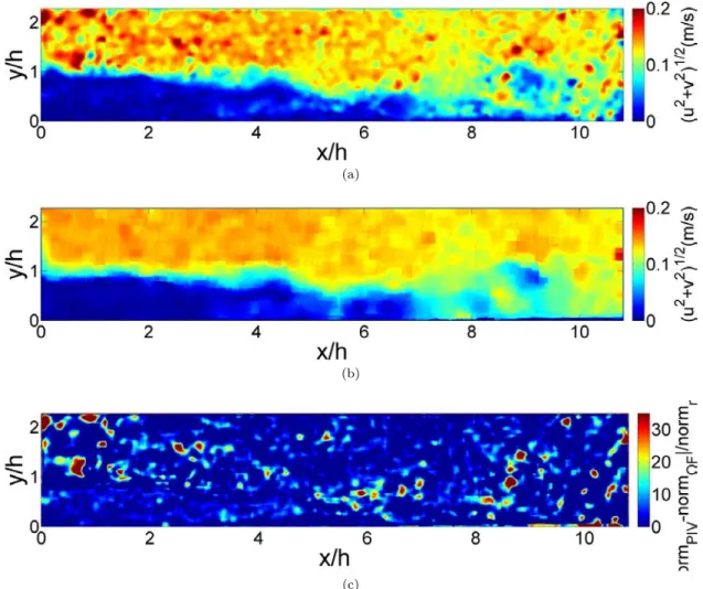
the time averaged velocity field. The ratio of negative to positive longitudinal velocity χ over a given time frame introduced by Simpson (1996) is most relevant for visualization. Figure 3.5 shows an example of χ for Reh= 1800.

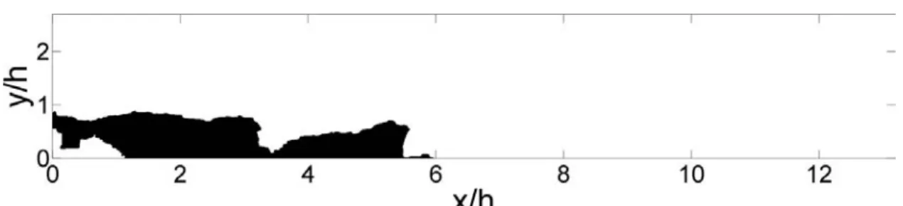
As a means of comparison figure 3.6 shows the corresponding recirculation region as defined in equation (3.2) for the time averaged field.

(47)

Figure 3.5: χ for Reh= 2700

Figure 3.6: Recirculation (in black) computed for the time averaged field, Reh= 2700

Equation (3.3) introduces recirculation intensity, the spatially averaged longitudinal ve-locity value inside Ar(t). This definition is useful when controlled and uncontrolled

recircu-lation area are of comparable size while recircurecircu-lation is less intense in one case. RI(t) = 1 Ar Z Ar −v(x, y, t) dA (3.3)

(48)

RI,f ield=< vx,y∈Ar(t)>t/maxx,y< v >t (3.4)

Figure 3.8: Time averaged, normalized recirculation intensity Reh= 1800

Figure 2.4b shows the different observations planes used for the following figures. More details on the similarities and differences between recirculation measurements in the vertical and horizontal plane are available in chapter 5.

Figure 3.9 shows recirculation time fraction for the available range of Reynolds numbers, the red line indicates χ = 0.5. Recirculation increases with Reynolds number up until a certain point where vortex shedding starts (Reh = 620) and gradually intensifies lowering

recirculation area until reaching an asymptote, this is coherent with what can be observed in figures 3.1a, 3.1b and 3.1c.

(a) Reh= 200

(b) Reh= 620

Figure 3.9: Recirculation time fractions for select Reynolds numbers, middle vertical plane, red line is χ = 0.5

(49)

(c) Reh= 1250

(d) Reh= 3250

Figure 3.9: Recirculation time fractions for select Reynolds numbers, middle vertical plane, red line is χ = 0.5

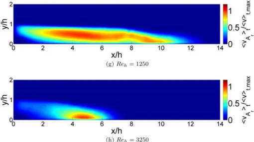
Figure 3.10 shows corresponding time averaged, normalized recirculation intensity. For high Reynolds numbers recirculation intensity is concentrated around the reattachment area, while lower free-stream velocity flows feature a spread out recirculation.

(50)

(g) Reh= 1250

(h) Reh= 3250

Figure 3.10: Time averaged, normalized recirculation intensity for select Reynolds numbers, middle vertical plane

Figure 3.11i shows maximum recirculation intensity as a function of Reh. Recirculation

intensifies linearly with free-stream velocity. This is in stark contrast to the evolution of recirculation size (length, area, volume). The same can be said about maximum fluctuating kinetic energy displayed in figure 3.11j.

(i) Maximum recirculation intensity as a function of Reh

(j) Maximum time averaged fluctuating kinetic energy y as a function of Reh

Figure 3.11

Figure 3.12 shows corresponding time averaged kinetic energy < k >tas a function of Reh,

with the instantaneous fluctuating kinetic energy k = √u02_{+ v}02 _u0 _{and v}0 _{are fluctuating}

longitudinal and vertical velocity. Prior to Reh = 620 the high fluctuating kinetic energy

region is due to flapping of the shear layer, for higher Reynolds numbers vortex shedding is responsible for the majority of fluctuating kinetic energy in the flow.

(51)

(a) Reh= 200

(b) Reh= 620

(c) Reh= 1250

(d) Reh= 3250

Figure 3.12: Time averaged fluctuating kinetic energy field for select Reynolds numbers Figure 3.13 shows velocity amplitude snapshots as a function of Reh. These snapshots

are meant to give a qualitative representation of the instantaneous flow for select Reynolds numbers. They offer a contrast to the much more common time-averaged representation.

(52)

(a) Reh= 200

(b) Reh= 620

(c) Reh= 1250

(d) Reh= 3250

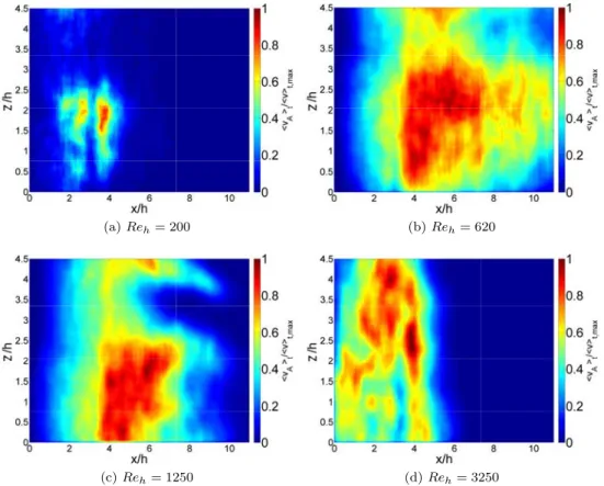
Figure 3.13: Instantaneous velocity amplitude snapshots for select Reynolds numbers Figure 3.14 shows the flow in the middle horizontal plane, the red line indicates χ = 0.5. In this configuration the camera is placed above the step. Recirculation evolution corroborates what has been observed in the vertical plane. This is noteworthy as it guarantees control of the vertical plane recirculation has the same time-averaged effects in the transversal direction. In practice vertical recirculation is a good representative of the transversally averaged recirculation. However if actuation is non transversally homogeneous, measuring recirculation in the horizontal plane is necessary for effective control.

(53)

(a) Reh= 200 (b) Reh= 620

(c) Reh= 1250 (d) Reh= 3250

Figure 3.14: Recirculation time fractions for select Reynolds numbers, middle horizontal plane (y=h/2), red line is χ = 0.5

Figure 3.15 shows time averaged, normalized recirculation intensity in the middle hori-zontal plane. As with the vertical plane, recirculation intensity closely follows recirculation time fractions. For the uncontrolled flow both quantities are equivalent.

(54)

(a) Reh= 200 (b) Reh= 620

(c) Reh= 1250 (d) Reh= 3250

Figure 3.15: Time averaged, normalized recirculation intensity for select Reynolds numbers, middle horizontal plane

3.3 3D: recirculation volume

The definitions of Ar and RI are easily expanded to 3D. Ar(t) becomes Vr(t) a measure of

recirculation volume described in equation (3.5).

Vr(t) =

V

H(_{−v(t))(x, y, z) dV} (3.5)

RI(t) conserves its notations and interpretation becoming, (3.6):

RI(t) = 1 Vr Vr −v(x, y, z, t) dV (3.6) The definition for χ is also identical. Figure 3.16 shows the iso-surface for v(x, y, z, t) = 0 for a 3D experimental velocity field at varying Reynolds numbers. This iso-surface delimits the volume defined in (3.5). The data were obtained using 3D particle tracking velocimetry. Unfortunately it is not yet possible to take these measurements in real-time. These results are presented to illustrate a possible next step for optical based flow control.

(55)

Flow control using optical sensors

HAL Id: tel-01150428

https://tel.archives-ouvertes.fr/tel-01150428

Submitted on 11 May 2015

Flow control using optical sensors

Nicolas Gautier

To cite this version:

Nicolas Gautier. Flow control using optical sensors. Mechanics of the fluids [physics.class-ph].

Uni-versité Pierre et Marie Curie - Paris VI, 2014. English. �NNT : 2014PA066640�. �tel-01150428�

Ecole doctorale: Sciences m´

ecaniques, acoustique, ´

electronique & robotique

(UPMC)

ESPCI, Laboratoire PMMH

Flow control using optical

sensors

(Contrˆ

ole d’´

ecoulement par capteurs optiques)

Nicolas Gautier

Th`ese de doctorat de Physique

Dirig´

ee par Jean-Luc Aider

Jury

Dr. Fran¸cois Lusseyran (Rapporteur)

LIMSI

Dr. Denis Sipp

(Rapporteur)

ONERA

Dr. Philippe Guibert

(Examinateur)

UPMC

Dr. Azeddine Kourta

(Examinateur)

PRISME

Dr. Bernd Noack

(Examinateur)

PPRIME

0.1

Abstract

0.3

Preface

Contents

I

Introduction

10

II

Results

41

Part I

Chapter 1

Introduction

1.1

Flow control

1.2

Closed-loop control

1.2.1

Adaptive control

1.2.2

Model based control

1.2.3

Machine learning

1.3

The special case of separated flows and the

back-ward facing step geometry

1.4

Optical sensors

1.5

Actuation

1.6

Control of the recirculation past a backward facing

step

1.7

Thesis organization

Bibliography

Chapter 2

Experimental setup

2.1

Hydrodynamic channel

2.2