HAL Id: halshs-01103359
https://halshs.archives-ouvertes.fr/halshs-01103359
Submitted on 27 May 2020
HAL is a multi-disciplinary open access
archive for the deposit and dissemination of sci-entific research documents, whether they are pub-lished or not. The documents may come from teaching and research institutions in France or abroad, or from public or private research centers.
L’archive ouverte pluridisciplinaire HAL, est destinée au dépôt et à la diffusion de documents scientifiques de niveau recherche, publiés ou non, émanant des établissements d’enseignement et de recherche français ou étrangers, des laboratoires publics ou privés.
Mediterranean watershed (Languedoc, France)
Jean-Baptiste Paroissien, Frédéric Darboux, Alain Couturier, Benoît Devillers,
Florent Mouillot, Damien Raclot, Yves Le Bissonnais
To cite this version:
Jean-Baptiste Paroissien, Frédéric Darboux, Alain Couturier, Benoît Devillers, Florent Mouillot, et al.. A method for modeling the effects of climate and land use changes on erosion and sustainability of soil in a Mediterranean watershed (Languedoc, France). Journal of Environmental Management, Elsevier, 2015, 150 (1), pp.57-68. �10.1016/j.jenvman.2014.10.034�. �halshs-01103359�
Version postprint
A method for modeling the effects of climate and land use
changes on erosion and sustainability of soil in a
Mediterranean watershed (Languedoc, France)
Paroissien Jean-Baptistea, b, Darboux Frédérica, Couturier Alaina, Devillers Benoitc, MouillotFlorentd, Raclot Damiene, Le Bissonnais Yvesf
aINRA, UR0272, UR Science du sol, Centre de recherche Val-de-Loire, CS 40001,F-45075 Orléans Cedex 2,
France
bINRA, US1106 InfoSol, Centre de recherche Val-de-Loire, CS 40001,F-45075 Orléans Cedex 2, France
cCNRS, Archéologie des Sociétés Méditerranéennes (ASM), UMR 6573, UMR 5140,Université Paul Valéry,
France
dIRD, UMR CEFE, 1919 route de Mende, 34293 Montpellier Cedex 5, France
eIRD, Laboratoire d’étude des Interactions Sol-Agrosystème-Hydrosystème, UMR LISAHINRA-IRD-SupAgro, 2
Place Viala, F-34060 Montpellier, France
fINRA, Laboratoire d’étude des Interactions Sol-Agrosystème-Hydrosystème, UMRLISAH INRA-IRD-SupAgro,
2 Place Viala, F-34060 Montpellier, France
______________
Abstract
Global climate and land use changes could strongly affect soil erosion and the capability of soils to sustain agriculture and in turn impact regional or global food security. The objective of our study was to develop a method to assess soil sustainability to erosion under changes in land use and climate. The method was applied in a typical mixed Mediterranean landscape in a wine-growing watershed (75 km2) within the Languedoc region (La Peyne, France) for two
periods: a first period with the current climate and land use and a second period with the climate and land use scenarios at the end of the twenty-first century. The Intergovernmental
Panel on Climate Change A1B future rainfall scenarios from the Météo France General circulation model was coupled with four contrasting land use change scenarios that were designed using a spatially-explicit land use change model. Mean annual erosion rate was estimated with an expert-based soil erosion model. Soil life expectancy was assessed using
soil depth. Soil erosion rate and soil life expectancy were combined into a sustainability index. The median simulated soil erosion rate for the current period was 3.5 t/ha/year and the soil life expectancy was 273 years, showing a low sustainability of soils. For the future period with the same land use distribution, the median simulated soil erosion rate was 4.2 t/ha/year and the soil life expectancy was 249 years. The results show that soil erosion rate and soil life expectancy are more sensitive to changes in land use than to changes in precipitation. Among
the scenarios tested, institution of a mandatory grass cover in vineyards seems to be an efficient means of significantly improving soil sustainability, both in terms of decreased soil
erosion rates and increased soil life expectancies.
Keywords: Climate change; Soil erosion; Land use change; Modeling; Soil sustainability
1. Introduction
Soil is an essential resource for the food chain and our society. Soil formation is a slow process, while soil destruction can be rapid. Hence, soil is considered a non-renewable
Version postprint
resource, and its sustainability is important. Among the threats to soil is erosion, which is a natural phenomenon that can be impacted by global change (Walker, 1994).
One of the most direct impacts of climate change could be an increase in heavy precipitation (IPCC, 2008) and studies on soil erosion have suggested that increased rainfall amounts and intensities will lead to greater rates of erosion unless protection measures are taken
(Kundzewicz et al., 2007). Several studies have recently performed erosion modeling under climate change to assess potential future environmental problems. These studies have mostly used continuous hydrological and erosion models (see review of Nunes and Nearing (2011)) and have generally been restricted to investigating only the direct impacts of climate change (changes in rainfall and temperature). Except a few contributions (i.e. O’Neal et al., 2005, Lesschen et al., 2007, Routschek et al., 2014) the vast majority of previous and present studies continue to neglect the changes in land use and management (Mullan et al., 2012). However, climate change forces land use shift (Rounsevell and Reay, 2009). Changes in both rainfall patterns and in land use due to human drivers (e.g., macroeconomics, technological changes, social trends and governance structures) could be affect soil erosion and hence, soil
sustainability. In an agricultural context, soil erosion could be strongly affected by changes in crop system (Kosmas et al., 1997), crop management (O’Neal et al., 2005) and cultural practices (Battany and Grismer, 2000; Loughran and Balog, 2006).
Currently, many methods of soil erosion assessment have been developed that can be used to create environmental and land use management plans. The latter rely on the concepts of soil erosion hazard which addresses the probability of the soil erosion phenomena. Hazard maps are produced at different scales (e.g., Le Bissonnais et al., 2002; van Rompaey et al., 2003) and can be based on empirical and expert models such as USLE (Universal Soil Loss Equation), MESALES (Modèle d’Evaluation Spatiale de l’Aléa Erosion des Sols) ( Bissonnais etLe al., 2002) and PESERA (Pan-European Soil Erosion Risk Assessment) (Kirkby et al., 2004).
However, this type of maps are often express the soil loss rate in t/ha/year, which is readily understood by erosion specialists but not by decision makers. Hence, to communicate with decision makers, there is a need for a scientifically-sound and easily-understood, index of soil erosion risk. The soil erosion risk is the combination of soil vulnerability and soil erosion hazard) (Taubenböck et al., 2008). The term “risk” is often described as “hazard” or “danger” and these terms are often used interchangeably, leading to some confusion
(Schneiderbauer, 2007). In fact, maps of soil erosion risk are not as common as erosion hazard maps, and only few studies have been dedicated to the assessment of soil erosion risk, though related concepts such as soil loss tolerance (Stamey and Smith, 1964) and soil lifetime (Sparovek and Schnug, 2001) are used. These two concepts use the vulnerability of soil depth to assess soil erosion risk, and soil is considered to be an economic resource. Several basic soil functions (e.g., soil fertility and carbon storage) can be depleted, degraded or destroyed by accelerated soil erosion (Lal, 2003). The soil is also closely connected to the culture and civilization of ethnic groups living in a certain place (e.g., their religion, livelihood and health) (Minami, 2009). Thus, it is important to consider the soil as a patrimonial resource when assessing soil erosion risk: the soil should be protected for itself, ensuring that it will support all of its current and future functions.
The purpose of this study is to overcome the above-mentioned difficulties. This work tests the hypotheses that combining climate and land use changes (1) improves the assessment of soil sustainability and (2) leads to information suitable for decision-making. The study is based on
Version postprint
the representative expected future rainfall years simulated by a General Circulation Model (GCM), ARPEGE Météo France, and on two chained numerical models. The first numerical model provides a model of land use change with land use scenarios and feeds the second, a model of soil erosion by overland flow.
The approach is applied in a watershed located in the Mediterranean area which is one of the areas most vulnerable to climate change (Giorgi and Lionello, 2008) and where most erosion studies showed an estimated soil loss rates exceeding the soil formation rates (Kosmas et al., 1997).
2. Study area
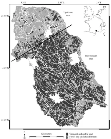
The Peyne watershed is located on the plain of the Hérault River, 60 km west of the city of Montpellier (France) (Fig.1). The watershed covers a surface area of approximately 75 km2.
The upstream area is hilly and mainly covered by shrublands and forests with little arable land. The downstream area has gentler topography and is mostly covered by vines (75 %) and cereals (20 %) (Biarnès et al, 2009). The climate is Mediterranean sub-humid with a long dry season. The average annual temperature is 14°C, and annual rainfall varies between 400 and 1400 mm with two main rainy periods (spring and autumn), in addition to potentially high-intensity rainfalls in summer.
Figure 1: Location of the study area with main land use of Peyne watershed, the black line
delineates the upstream zone from the downstream zone.
Version postprint
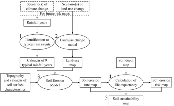
The proposed method enables assessment of soil erosion risk for current (2000-2010) and future (2071-2100) climate and land use scenarios and can be broken down into five steps (Fig. 2). Precipitation levels are set during step 1, while land use is defined in step 2. During step 3, soil erosion is modeled and a map of soil erosion rate is produced. Step 4 computes the life expectancy of soil, and step 5 produces a map of soil sustainability. The method is applied to the Peyne watershed (France), but it is designed to be flexible (i.e., to be usable with other data and numerical models).
Figure 2: Flow chart of tasks to assess soil erosion risk. Step 1 sets rainfall levels, step 2 defines
land use, step 3 models soil erosion, step 4 calculates soil erosion risk, and step 5 calculates soil sustainability.
3.1. Current and future precipitation
3.1.1. Current precipitation
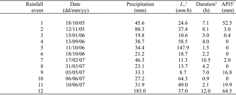
We developed a method for erosion risk assessment using soil erosion modeling in a context of short-term monitoring data availability. This method aims to account for the inter-annual variability of precipitation and takes into consideration a reduced/limited number of simulated rainfall events and simulated years. Out of the 15 years of rainfall records available for the watershed, data from years 2005, 2006 and 2007 were available with an hourly time step. This 3-year period was used to select 12 typical and potentially-erosive rainfall events. Eleven rainfall events with contrasting characteristics in terms of cumulative rainfall, maximum rainfall intensity and duration (Table 1) covered the range of observed rainfall conditions. Because extreme rainfall events were unlikely to be measured during this 3-year timeframe, a twelfth event was added (T12) to represent a potential extreme rainfall. This latter rainfall event was defined as the maximum precipitation recorded for a single rainfall event during the 15-year-long record. Nine typical yearly rainfall sequences were simulated using the
following three steps:
Version postprint
From the 15-year dataset (with a daily time step), the 3 rainiest years, the 3 years closest to the median total rainfall amount, and the 3 driest years were selected. Selection of 9 years of data enabled inter-year variability to be accounted for to some extent.
Matching all rainfalls with the 12 typical and potentially-erosive rain events:
Considering that rainfall events with a cumulative precipitation lower than 20 mm do not cause overland flow and erosion in the study area, these events were discarded from the 9-year record. The characteristics of the remaining rainfall events were then compared to the 12 typical rain events using a principal component analysis. Each rainfall event in the 9-year record was matched with one typical rain event.
Building a monthly calendar:
Each typical precipitation year was characterized by a monthly combination of typical rainfall events.
Rainfall Date Precipitation Imax1 Duration2 API53
event (dd/mm/yy) (mm) (mm/h) (h) (mm) 1 18/10/05 45.6 24.6 7.1 52.5 2 12/11/05 88.3 37.4 8.1 3.0 3 15/01/06 19.8 10.6 3.0 0.4 4 13/09/06 38.7 58.5 4.0 0 5 11/10/06 34.4 147.9 1.5 0 6 18/10/06 21.2 18.7 2.2 0 7 17/02/07 46.3 11.3 10.5 2.0 8 31/03/07 23.1 13.7 4.2 0 9 03/05/07 33.1 8.7 7.0 16.8 10 06/06/07 27.2 64.3 0.9 0 11 10/06/07 31.9 49.0 2.1 19.9 12 183.0 37.0 12.0 64.5
1Maximum intensity. 2Effective duration at 2 mm/h. 3Antecedent precipitation index (5 days).
Table 1: Rainfall event characteristics used for the construction of the 9 representatives rainfall
years.
3.1.2. Future precipitation
We used climate scenarios from the ARPEGE v. 3.0 GCM at 50 km resolution for the Mediterranean area (Gibelin and Déqué, 2003) delivered over a 30-year period for both the present (ARPEGEref, atmospheric CO2 360 ppm) and future (ARPEGEfut, 720 ppm IPCC
scenario A1B). GCMs are able to simulate climate variables on a daily time step, but their spatial resolution is coarse. Among all available GCMs, ARPEGE provides the finest resolution for the region because it is built on a spatially heterogeneous global grid with an increasing resolution centered over the Mediterranean basin. However, within the 50 km resolution grid cells, rainfall patterns are still highly variable. Indeed, ARPEGE rainfall simulations generally did not fit rain gauge data, resulting in biases both in terms of annual and seasonal rainfall amounts. These acknowledged biases prevent direct application of GCM
Version postprint
outputs for impact studies. To account for this bias, we selected the quantile-mapping method (Boe et al., 2007), previously applied for the region by Ruffault et al. (2014), from among available climate data preprocessing techniques (Déqué, 2007). The method compares the frequency distribution of different intensities of individual climatic events with a reference dataset and observations. The monthly cumulative distribution function (CDF) of
ARPGEGEref was first compared to the CDF of the observed rainfall time series to generate a correction value for each quantile. These monthly correction functions were then used to correct daily rainfall amount from the projected climate scenario quantile by quantile (see Ruffault et al. (2014) for more details).
3.2. Current and future land use
3.2.1. Current land use
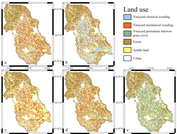
The current land use map was established by combining field survey and interpretation of IGN (French National Institute of Geography) ortho-photographs from the spring of 2005. The land use classes were vineyard (vine and orchard), arable land, forest (abandoned land, shrub and pine forest) and urban (road network, natural and artificial hydrologic network). The percentages of agricultural practices in vineyards are given in Biarnès et al. (2004): 62.5% mechanical weeding, 27.5% chemical weeding and 10% permanent interrow grass cover. However, no map is available. To account for these practices, they were assigned randomly to the land use vineyard with the prescribed percentages.
3.2.2. Future land use
Based on the current land use, future land use scenarios were built using the Conversion of Land Use and its Effects at Small regional extent model (CLUE-S) (Verburg et al., 2002). CLUE-S has been used in many contexts, with a growing interest for global change (Verburg and Denier van der Gon, 2001; Castella and Verburg, 2007; Schulp et al., 2008) and soil erosion (Lesschen et al., 2007; Ward et al., 2009). CLUE-S builds a binary logistic regression between the present land use distribution and a selected panel of contributive variables
defined a priori by the user. According to a prescribed change in the land use classes, CLUE-S distributes each land use across the landscape according to a statistical model built on the current situation and the distance to the initial distribution. In addition, a set of functions is specified by the user to address a hierarchic organization of land use change: a spatial connectivity between the destinations of land use change and spatial policies (e.g. nature reserve area) can be incorporated in the land use allocation.
Driving factors. Table 2 summarizes the factors used for statistical analysis. Scores for each predictor were obtained from the beta coefficients assigned by the binary logistic model. The model of driving factors is validated by the Receiver Operating Characteristic method (ROC) (Pontius and Schneider, 2001). This method evaluates the performance of the regression model by evaluating the specificity of the regression (capacity to predict the proper land use) and the sensitiveness of the regression (capacity not to predict an improper land use). The Area Under Curve allows evaluation of the probability that the model will correctly predict land uses.
Version postprint
Driving factor Description
Land use Based on field observation and photo-interpretation (IGN, 2005)
Altitude Digital elevation model (DEM) based on 1:250,000
contour lines, resolution 10 m2 (IGN, 1989)
Slope Derived from DEM
Slope > 10% Derived from DEM
Topography position indice Derived from DEM with ArcMap script of Jenness (2005) Geomorphologic classification Derived from DEM with ArcMap script of Jenness (2005)
Table 2: Driving factors used for the binary logistic regression.
Land use change scenarios. Land use changes on the Peyne watershed are expected to
follow the trends of the Mediterranean region and reflect the specificities of its status as a wine-growing area. Four scenarios were considered. The first three scenarios are based on the Convulsive changes, Big is beautiful and Knowledge is king scenarios in Kok et al. (2006). These scenarios put the evolution of land use in a context that accounts for economic, social and climatic considerations. The fourth scenario was designed to test the efficiency of an environmental law.
Accentuation:
Accentuation expresses irreversible climate change acceleration with the formation of permanent desert in southern Europe. In this scenario, chemical weeding in vineyards develops to limit water and nitrogen competition with weeds, and the surface of arable land increases, while forests remain almost unchanged.
Production:
Production reflects increasing market liberalization, with an expansion of the
European Union and merging of multinational companies. Arable land expands greatly and replaces parts of vineyards and forests.
Protection:
Protection reflects the rapidly increasing importance of information and
communication technology and the development of many important inventions (e.g., high-yielding crop varieties). For the Peyne watershed, agricultural practices become more environmentally friendly. Forests are protected, and permanent interrow grass cover develops in vineyards (particularly for plots with chemical weeding).
Environmental law:
This land use change is based on the application of a hypothetical law derived from the framework of the soil protection directive (Commission of the European
Communities, 2006). For the Peyne watershed, it translates into permanent interrow grass cover for all vineyards, while surface areas in forests and arable land remain unchanged.
CLUE-S simulates final future land uses from these scenarios at the end of the 21st century. Intermediate land uses are not considered.
Version postprint
3.3. Soil erosion rate
3.3.1. Soil erosion model
The Sealing and Transfer by Runoff and Erosion related to Agricultural Management
(STREAM) model uses a raster-based approach to calculate the spatial distribution of runoff and soil erosion at the time scale of a rain event (Cerdan et al., 2002b; Souchère et al., 2005). This expert-based model assumes that the main controlling factors of infiltration, overland flow and erosion at the field-scale are soil surface characteristics, namely crusting, surface roughness, cover (vegetation and residues) and initial moisture content. These characteristics are set for each land use over the watershed. Then, infiltration rates are assigned to each land use. For each rainfall event, the overland flow network is computed using a digital elevation model, and water is routed on this network. Finally, soil erosion is simulated by the modules of sheet erosion and rill erosion (Cerdan et al., 2002a):
1. The module of sheet erosion assigns a potential sediment concentration according to the soil surface characteristics.
2. The module of rill erosion estimate soil erosion based on parameters that control overland flow velocity and soil erodibility (slope gradient, vegetation type, vegetable cover, soil roughness, crusting).
3.3.2. Adaptation of STREAM
The model parameters were adapted to local land uses and soil properties. A monthly calendar of soil surface characteristics was built using data from long-term monitoring of a
sub-watershed (Moussa et al., 2002; Corbane et al., 2008). Sub-sub-watersheds (mean surface area of 67 ha) were delineated based on the available hydrological and road networks. The
distribution of soil erosion rates was calculated for each sub-watershed, and the value corresponding to the 9th decile of this distribution (10% of the sub-watershed area has higher
soil erosion rates) was assigned. In comparison to the use of average or maximum values, use of the 9th decile accounts for the existence of high soil erosion rates (i.e., possible high-risk
areas within a sub-watershed) and avoids reliance on the value of a single cell. This allows visualization of a sub-watershed containing a significant proportion of high erosion rates without sensitivity to extreme values that may result from an extremely limited surface area (e.g., a single cell of 100 m2).
3.4. Life expectancy
In this work, the soil sustainability is defined from a patrimonial point of view. The soil should be protected for itself, ensuring that it will support all of its current and future functions. This concept implies to evaluate the duration for which a system is able to cope with the risk. In the case of erosion, sustainability can be represented by the life expectancy of soil. In the present study, we chose to determine the duration before complete soil
disappearance (i.e., the amount of time before erosion removes all of the soil at a given location). This is based on Sparovek and Schnug (2001), who defined the lifetime of a soil as “ a time until a minimum soil depth needed for sustaining crop production is reached”. We did not account for soil formation because rates are largely unknown and are generally considered to be very low compared to soil erosion rates (Gobin et al., 2006). The following definition of
Version postprint
life expectancy was used, where life expectancy is expressed in years, soil depth is expressed in meters, and soil erosion rate is in m/year:
(1) This equation is valid only for positive soil erosion rates. For a null erosion rate or a negative soil erosion rate (i.e., sedimentation), life expectancy is infinite. Because STREAM gives soil erosion rates in t/ha/year, using a constant bulk density of 1510 kg/m3 (Lagacherie
et
al., 2006), the same bulk density was used to convert the t/ha/year into m/year. The present soil depth map was established using intensive field survey and pedologic expertise
(Coulouma, 2009). A soil depth (considering A, B and C horizons) was assigned to each pedologic unit. First, life expectancy was computed for each cell, taking into consideration the soil depth map and the soil erosion rate. Using a procedure similar to the one used for soil erosion rate, life expectancy was summarized at the sub-watershed scale. However, the first decile was used for life expectancy (i.e., the sub-watersheds with a low soil life expectancy that may require further attention were put forward).
3.5. Soil sustainability
Soil erosion rate does not relate directly to sustainability because it refers to how much soil is eroded without considering the initial amount of soil. However, soil erosion rate is
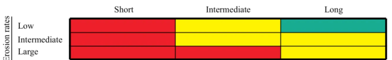
informative with regards to how much soil is transported downslope and downstream. Areas with large erosion rates are thus likely to threaten the sustainability of streams and rivers (i.e., they have off-site effects). Complementarily, life expectancy is concerned with the durability of soil functions on-site. Hence, both soil erosion rate and life expectancy contain information about sustainability. A high sustainability implies a low soil erosion rate and a long life expectancy. Sustainability can be mapped using threshold values. We suggest using threshold values of 100 and 1000 years as the limits between short, intermediate and long life
expectancies and 1 and 3 t/ha/year as the limits between low, intermediate and high soil erosion rates. Maps of soil sustainability can be built based on these criteria (Fig. 3).
Figure 3: Assessment of soil sustainability using both erosion rate and life expectancy. 3.6. Statistical analysis
The nonparametric Kruskal-Wallis test with corrections for multiple testing was used to check for differences in erosion rate or life expectancy among land uses and among scenarios. When test results are significant, there is at least one difference between two of the land uses (or scenarios). This test is similar to a single-factor analysis of variance but does not assume a normal distribution. Identification of the differences among land uses (or scenarios) was
Version postprint
performed using the Chi-squared test. For all tests, a significant threshold of 5% was
considered. All of these analyses were performed using R (R Development Core Team, 2012), and spatial analysis and mapping were carried out using the GRASS GIS (GRASS
Development Team, 2012) and Generic Mapping Tools software (Wessel and Smith, 1991).
4. Results
4.1. Current and future precipitation
4.1.1. Current precipitation
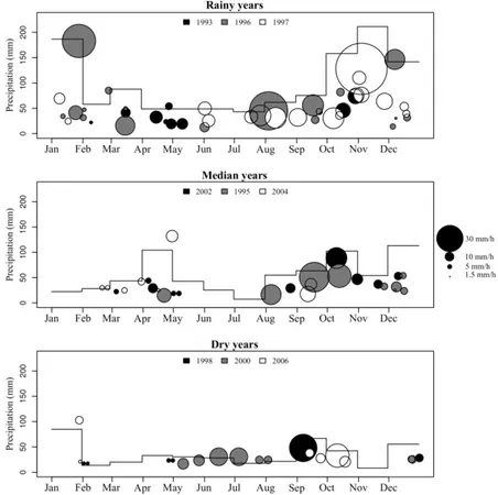
Figure 4 shows the nine rainfall years (divided into rainy, median and dry years) re-constructed using the 12 typical rainfall events. Rainy years are characterized by a large number of rainfall events distributed in winter and autumn. During these two seasons, the rainfall events are characterized by higher rain amounts and intensities than the rainfall events in spring and summer. Median and dry years show fewer rainfall events than rainy years, and these rainfall events have lower rain amounts and intensities. Median and dry years differ from each other in total precipitation and annual distribution of rainfall events: median years show more precipitation in autumn and spring, while dry years show more precipitation in late summer and early winter.
Figure 4: The 9 rainfall years constructed from the typical rainfall events. The mean monthly
precipitation over the selected 3 years is represented by a black line. Each typical rainfall event is represented by a spot chart whose color denotes the year and size denotes the mean rainfall intensity.
Version postprint
The total simulated precipitation levels for the current and future periods are 438 mm and 408 mm, respectively (i.e., a decrease of 7% is projected) (Fig. 5). Current climate patterns show similar precipitation levels in spring, summer and autumn, and higher precipitation levels in winter. The differences between winter and the other seasons increase when future precipitation levels are considered; an increase of 49 mm is projected for winter, while a decrease of approximately 27 mm is projected for the other seasons.
Figure 5: Precipitation levels by seasons for current and future climates. 4.2. Land use change
The beta coefficient of the binary logistic regression is the highest for the slope and the slope > 10% factors (Table 3), indicating that slope is an important determinant for land use
distribution. Amount of arable land increases when the slope decreases (negative value), while forests mostly occur when the slope increases (positive value). Values of the other potential driving factors are low, indicating their inability to predict the spatial pattern of land use. The area under the curve (AUC) can range between 0.5 (completely random prediction) and 1 (completely deterministic prediction). AUC is large for forests (0.83) but is much lower for the other land uses, with values ranging from 0.56 to 0.66. Figure 6 shows the current and predicted land use maps for the four scenarios. For all scenarios, arable land and vineyards remained mostly in the downstream area of the Peyne watershed, and forests remained mostly in the upstream area. Only the Production scenario induced a large change in both the
upstream and downstream areas, with an increase in arable land in the downstream area and a sharp decrease in vineyards in the upstream area.
Version postprint
Driving factors
Vineyard
Forest Arableland Chemical Mechanical Permanentinterrow
weeding weeding grass cover
Altitude -0.008 -0.005 0.012 -0.008 Slope -0.10 -0.13 -0.046 0.16 -0.073 Slope >10% 0.13 0.40 TPI1 -0.019 -0.011 0.058 GC2 0.045 0.028 -0.21 AUC3 0.58 0.66 0.56 0.83 0.60
1Topography position indice. 2Geomorphologic
classification. 3Area under the curve.
Table 3: Driving factors and the standardized beta coefficients for each land use type
Figure 6: Maps of land uses. (a) Current, (b) Accentuation scenario, (c) Production scenario, (d)
Version postprint
4.3. Erosion rate maps and distributions
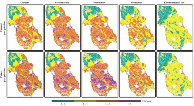
All of the erosion rate maps show a similar pattern, with a sharp contrast between the upstream and downstream areas (Fig. 7): the upstream area has mostly low erosion rates, while the downstream area has high erosion rates. The maps are similar in their spatial
distribution of erosion rates, except for those produced using the Environmental law scenario, which display much lower erosion rates, especially in the downstream area. Erosion rate distributions are significantly different for all scenarios (p-value < 0.005), except for between the Current and Accentuation scenarios for current precipitation (Fig. 8a). For example, the median soil erosion rate for the current period is 3.5 t/ha/year while for the future period with the same land use distribution, it is 4.2 t/ha/year. Overall, the Accentuation and Production scenarios increase the median erosion rate, while Protection and Environmental law scenarios decrease it. Compared to the present situation, the Production scenario with the future
precipitation rate causes the greatest increase in soil erosion rate. Only the Environmental law scenario decreases the median erosion rate sharply. For a given land use scenario, the future precipitation consistently gives a higher median erosion rate than the current precipitation. The largest effect on the median erosion rate is found in the Production scenario. When median values are considered, the differences between the current and future precipitation levels for a given land use are lower than the differences between land uses (for the same precipitation). Thus, land use change has a greater impact on soil erosion rate than precipitation change. When the distribution of soil erosion rates for each land use is considered (Fig. 9a), vineyards with permanent interrow grass cover and forests have
significantly lower erosion rates (mean of 2.8 and 2.0 t/ha/year, respectively) than vineyards with chemical weeding, vineyards with mechanical weeding and arable land (mean erosion rates of 4.4, 4.8 and 4.0 t/ha/year, respectively).
Version postprint
Figure 8: Boxplot of current soil erosion rate (a) and life expectancy (b) depending on land use
scenarios, for current and future precipitation. The plots show the median, the 25th and 75th
percentile scores (boxes). Outliers are not drawn.
Figure 9: Boxplot of current soil erosion rate (a) and life expectancy (b) for the main land uses.
The plots show the median, the 25th and 75th percentile scores (boxes). Outliers are not drawn.
4.4. Life expectancy maps and distributions
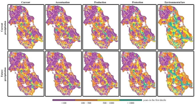
The maps of life expectancy do not show a clear upstream-downstream contrast (Fig. 10). The maps are similar, except for the Environmental law scenario, which displays more areas with a long life expectancies. Life expectancy distributions are not always significantly different (Fig. 8b): the Current situation and Accentuation scenarios (with both current and future precipitation) and the Production scenario with current precipitation have the same
distribution of life expectancies. The median simulated soil life expectancy for the current period is 273 years while for the future period with the same land use distribution, it is 249 years. For current precipitation, life expectancy is longer in the Protection and
Environmental law scenarios. In the Production, Protection and Environmental law scenarios, future precipitation levels lead to a decrease in life expectancy. Only the Protection and the Environmental law scenarios show a large increase in life expectancy.
Version postprint
Figure 10: Maps of soil life expectancy for land use scenarios and current and future
precipitations.
4.5. Soil sustainability maps
Soil sustainability is similar when current and future precipitation levels are considered, emphasizing that land use is the primary controlling factor (Fig. 11). The Accentuation and Production scenarios keep the soil sustainability low. The Protection scenario improves the sustainability, with limited development of areas of intermediate sustainability. Only the Environmental law scenario strongly improves sustainability: most of the watershed (82%) goes from low to intermediate sustainability, and a few areas (8%) achieve high sustainability.
Version postprint
Figure 11: Maps of soil sustainability for land use scenarios and current and future precipitations.
5. Discussions
5.1. Climate and land use scenarios
We used rainfall projections from ARPEGE GCM, which predicted a decrease of approximately 30% in summer precipitation levels in the region, a value in the range predicted by most climate models used across the Mediterranean Basin (Giorgi and Lionello, 2008). Bias correction remains a key challenge for local-scale applications, with significant differences seen in impact studies (Ruffault et al., 2014). We selected a rainfall-event approach to better capture changes in rainfall frequency and intensity that contribute to erosion processes (Quiquerez et al., 2008). Such approach was used by Ramos and Martínez-Casasnovas (2009) to evaluate erosive impact of rainfall events. However, because data availability is limited in numerous areas, we designed an alternative approach that does not require long-term rainfall records.
We then independently derived spatially-explicit land use scenarios that were suitable for decision-making based on typical land use trajectories from contrasting storylines. The low AUC values attributed to vineyard and arable land can be explained by the low topography contrast inside the downstream area (gentle landforms) and by the apparently-random allocation of vineyard cultural practices. The CLUE-S model was able to produce scenarios preserving the main feature of the Peyne watershed, i.e. the overall distribution of forest and cultivated land (vineyard and arable land) between the upstream and downstream areas. More deterministic projections could reveal the most probable land use distribution. An improved approach could include field ownership and soil degradation as feedback processes (Biarnès et al., 2004), climate change impact on vineyards and crop production and
distribution (Hannah et al., 2013), ecosystem sustainability under increasing drought, fire frequency (Mouillot et al., 2005) and the impact of land use policies (i.e. a new European
Version postprint
agricultural policy (López-Vicente et al., 2014)) (Stoate et al., 2009). For the implantation of a local management plan, a specific scenario for vineyard context can be developed. Indeed, the landscape effects of the EU Council Regulation policy for vineyards’ restructuring (Cots-Folch et al., 2006) could increase soil erosion problems (Ramos and
Martínez-Casasnovas, 2006) and the grubbing-up grants of vineyard and vineyard abandonment (Lieskovský et al., 2013) could have impacts on soil sustainability.
5.2. Model performance and limitations
The aim of this study was to develop a method to assess soil sustainability to erosion under changes in land use and climate. It was not to improve the soil erosion modeling. Hence we used a model (STREAM) that was previously validated in the same area (Ciampalini et al., 2012, David et al., 2014) with real field observations, leading to a robust estimation of soil erosion rates. For example, the long-term soil loss prediction (century scale) of Ciampalini et al. (2012) are corroborated by cumulative field-scale erosion measurements in the same area by Paroissien et al. (2010).
In our study, the average simulated soil loss for the watershed (4.2 t/ha/year) for the current precipitation and current land use is within the range of values measured in Europe (Cerdan et
al ., 2010). Indeed, the mean erosion rate simulated for arable land (4.0 t/ha/year) is very close to the one (3.6 t/ha/year) estimated by Cerdan et al. (2010). However, the mean erosion rate simulated for vineyards (3 t/ha/year) is lower than the erosion rate quantified
(10.5 t/ha/year) at the multi-decennial scale in the same study area (Paroissien et al., 2010). This discrepancy may be due to the influence of the connectivity between vineyard fields and to under-estimation of sedimentation rates by STREAM. More generally, the large spatial and temporal variability of soil erosion processes and the uncertainty associated with the input parameters (Jetten et al., 2003) could also explain the difficulties to compute soil erosion rates.
Another limitation of our approach is that our projections do not account for the potential impact of climate change on soil surface characteristics or for changes in agricultural practices (e.g., change in harvest date). European Environment Agency (2012) projections suggest a significant reduction in soil moisture in the Mediterranean region and earlier vine
development for 2020-2049 (Brisson and Levrault, 2010). Thus, competition between vine and grass would potentially increase, leading to a reduction in the use of interrow grass to prevent erosion. This issue should be examined further; permanent interrow grass cover could limit runoff during high-intensity rainfall, reduce erosion and allow optimal soil water uptake on slopes, thus delaying the desertification process and allowing continued cultivation.
5.3. Life expectancy and implications for sustainability
Estimation of life expectancy depends on erosion rate and soil depth estimates. Soil depth was estimated from a soil map combining A, B and C horizons. It could be argued that when the C horizon is the only one left, most of the soil functions have disappeared, so only the combined depths of A and B should be used. This should be decided on a case-by-case basis. The decision may also depend on the potentially adapted crops in the study area. In the present study, the C horizon was included due to the importance of vineyards in the area and the fact that vines can grow even if only the C horizon remains (unlike the cereal crops found on the arable land). The overall life expectancy would have been much shorter if the C horizon were not considered as it would be the case if cereals or other annual crops would replace vineyard.
Version postprint
Regardless of the set of horizons considered, soils with life expectancies lower than 100 years are without a doubt highly vulnerable. Their disappearance would threaten the entire
ecosystem and the environment and make the development of desertification and badlands likely. Soil conservation management at the watershed scale is usually based solely on the soil erosion rate (Foster et al, 2003). The present study complements this index with the soil life expectancy. While the soil erosion rate puts emphasis on soil loss, the soil life expectancy stresses the importance of soil durability, which relates more directly to the idea of
sustainability. Moreover, while erosion rate is understood by erosion specialists only, life expectancy is a familiar concept for non-specialists. Hence, presenting maps with life
expectancy expressed in years to stakeholders and decision makers could be more fruitful than presenting soil loss (expressed in t/ha/year) data. Because it is more easily-understood, life expectancy may be a better index than erosion rate, especially when on-site effects are considered. Erosion rate and life expectancy can be used concomitantly. When the erosion rate is large, it means an important amount of soil will be removed from the site, which could have consequences downslope or downstream. It also means that the upper horizon, often rich in nutrients, is being lost and is therefore unavailable for plant growth. Life expectancy considers the soil in its own right. A short life expectancy is a direct indicator that the sustainability of all soil functions is jeopardized and that the functions will disappear in the short-term. Hence, the two indices carry different and complementary information, and it is useful to combine them to assess the soil sustainability (Fig. 11). If a short life expectancy always translates into non-sustainability, only the combination of a low erosion rate and a long life expectancy ensures soil sustainability.
6. Conclusions
Based on the proposed method, the effect of land use change was much more significant than the effect of precipitation change in the Peyne watershed. The current soil sustainability is low in the study area. Among the studied scenarios, the application of an Environmental law prescribing permanent interrow grass cover for all vineyards was the only scenario that resulted in a significant increase in soil sustainability.
The developed approach address the issue of the impact of climate and land use changes on soil sustainability. It allows for the assessment of both the soil erosion risk and soil life expectancy for various land use scenarios and climate change scenarios. Soil erosion rate is used to assess mostly off-site effects. Life expectancy is directly linked with the durability of soils as a patrimonial resource. To account for both, soil erosion rate and soil life expectancy are combined into a sustainability index. Both soil life expectancy and the sustainability index can be used for long-term preservation of soil functions and can be readily understood by decision makers.
The method was designed to require a minimal amount of input data. The construction of rainfall years from a limited set of typical rain events reduced the number of necessary simulations and simplified the use of the soil erosion model. As applied here, the approach was based on the coupling of a land use change model (CLUE-S) and a soil erosion model (STREAM). However, the approach could be applied with other land use and erosion models, making it applicable to other areas (even out of the Mediterranean context) without substantial changes in the workflow.
Improvement of the approach could take into account spatial variability in soil formation rates, the potential impacts of climate change on soil surface characteristics and agricultural
Version postprint
practices (e.g., the interactions between climate and land use changes), and the modeling of additional variables such as the soil organic carbon dynamics.
Acknowledgments
This work was made possible by the financial support of the French National Research Agency through research project MESOEROS21 (ANR-06-VULN-012). We give special thanks to Cheng Chiv for her help in translating the manuscript and for comments.
References
Battany, M., Grismer, M., 2000. Rainfall runoff and erosion in napa valley vineyards: effects of slope, cover and surface roughness. Hydrological Processes 14, 1289—1304. Biarnès, A., Bailly, J., Boissieux, Y., 2009. Identifying indicators of the spatial variation of agricultural practices by a tree partitioning method: The case of weed control practices in a vine growing catchment. Agricultural Systems 99, 105 — 116.
Biarnès, A., Rio, P., Hocheux, A., 2004. Analyzing the determinants of spatial distribution of weed control practices in a languedoc vineyard catchment. Agronomie 24, 187—196. Boe, J., Terray, L., Habets, F., Martin, E., 2007. Statistical and dynamical downscaling of
the seine basin climate for hydro meterological studies. International Journal of Climatology 27, 1643—1655.
Brisson, N., Levrault, F., 2010. Climate change, agriculture and forests in France: simulations of the impacts on the main species. The Green Book of the CLIMATOR project (2007-2010). ADEME.
Casalí, J., Giménez, R., De Santisteban, L., Álvarez Mozos, J., Mena, J., Del Valle de Lersundi, J., 2009. Determination of long-term erosion rates in vineyards of Navarre (Spain) using botanical benchmarks. Catena 78, 12 — 19.
Castella, J., Verburg, P., 2007. Combination of process-oriented and pattern-oriented models of land-use change in a mountain area of Vietnam. Ecological Modelling 202, 410—420. Cerdan, O., Govers, G., Le Bissonnais, Y., Van Oost, K., Poesen, J., Saby, N., Gobin, A.,
Vacca, A., Quinton, J., Auerswald, K., Klik, A., Kwaad, F., Raclot, D., Ionita, I., Rejman, J., Rousseva, S., Muxart, T., Roxo, M., Dostal, T., 2010. Rates and spatial variations of soil erosion in Europe: A study based on erosion plot data. Geomorphology 122, 167— 177.
Cerdan, O., Le Bissonnais, Y., Couturier, A., Saby, N., 2002a. Modelling interrill erosion in small cultivated catchments. Hydrological Processes 16, 3215—3226.
Cerdan, O., Le Bissonnais, Y., Souchère, V., Martin, P., Lecomte, V., 2002b. Sediment concentration in interrill flow: interactions between soil surface conditions, vegetation and rainfall. Earth Surface Processes and Landforms 27, 193—205.
Ciampalini, R., Follain, S., Le Bissonnais, Y., 2012. Landsoil: a model for the analysis of erosion impact on agricultural landscape evolution. Geomorphology 175—176, 25—37. Commission of the European Communities, 2006. Proposal for a Directive of the European
Parliament and of the Council establishing a framework for the protection of soil and amending Directive 2004/35/EC. Technical Report. COM(2006) 232 final.
Version postprint
Corbane, C., Andrieux, P., Voltz, M., Chadoeuf, J., Albergel, J., Robbez-Masson, j., Zante, P., 2008. Assessing the variability of soil surface characteristics in row-cropped fields: The case of Mediterranean vineyards in Southern France. Catena 72, 79—90.
Cots-Folch, R., Martínez-Casasnovas, J., Ramos, M., 2006. Land terracing for new vineyard plantations in the North-Eastern Spanish Mediterranean region: Landscape effects of the eu council regulation policy for vineyards restructuring. Agriculture, Ecosystems and Environment 115, 88—96.
Coulouma, G., 2009. Map of soil depth for the Peyne. Technical Report. INRA, Laboratoire d’étude des Interactions Sols, Agrosystèmes, Hydrosystèmes. [in French]
David, M., Follain, S., Ciampalini, R., Le Bissonnais, Y., Couturier, A., Walter, C., 2014. Simulation of medium-term soil redistributions for different land use and landscape design scenarios within a vineyard landscape in Mediterranean France. Geomorphology 214, 10—21.
Déqué, M., 2007. Frequency of precipitation and temperature extremes over France in an anthropogenic scenario: Model results and statistical correction according to observed values. Global and Planetary Change 57, 16—26.
European Environment Agency, 2012. Climate change, impacts and vulnerability in Europe 2012. An indicator-based report. Technical Report. European Environment Agency. Kongens Nytorv 6 1050 Copenhagen K Denmark.
Foster, G.R., Yoder, D.C., Weesies, G.A., McCool, D.K., McGregor, K.C., Bingner, R.L., 2003. User’s Guide. Revised Universal Soil Loss Equation Version 2. RUSLE2. Technical Report. USDA-Agricultural Research Service. Washington, D.C., USA. Gibelin, A.L., Déqué, M., 2003. Anthropogenic climate change over the Mediterranean
region simulated by a global variable resolution model. Climate Dynamics 20, 327— 339.
Giorgi, F., Lionello, P., 2008. Climate change projections for the Mediterranean region. Global and Planetary Change 63, 90—104.
Gobin, A., Govers, G., Kirkby, M., 2006. Soil erosion in Europe. John Wiley & Sons Inc. Chapter Pan-European Soil Erosion Assessment and Maps. pp. 661—674.
GRASS Development Team, 2012. Geographic Resources Analysis Support System (GRASS GIS) Software. Open Source Geospatial Foundation. USA. URL: http://grass.osgeo.org.
Hannah, L., Roehrdanz, P., Ikegami, M., Shepard, A., Shaw, R., Tabor, G., Zhi, L., Marquet, P., Hijmans, R., 2013. Climate change, wine, and conservation. Proceedings of the National Academy of Sciences of the United States of America 110, 6907—6912. IGN, 1989. Bdtopo. URL: http://professionnels.ign.fr/bdtopo. IPCC, 2008. Climate change and water. Technical Report. Intergovernmental Panel on
Climate Change.
Jenness, J., 2005. Topographic Position Index extension for ArcView 3.x. Technical Report. Jenness Entreprise, Flagstaff, USA.
Jetten, V., Govers, G., Hessel, R., 2003. Erosion models: Quality of spatial predictions. Hydrological Processes 17, 887—900.
Version postprint
Kirkby, M., Jones, R., Irvine, B., Gobin, A., Govers, G., Cerdan, O., Van Rompaey, A., Le Bissonnais, Y., Daroussin, J., King, D., Montanarella, L., Grimm, M., Vieillefont, V., Puigdefabregas, J., Boer, M., Kosmas, C., Yassoglou, N., Tsara, M., Mantel, S., van Lynden, G., Huting, J., 2004. Pan-European Soil Erosion Risk Assessment: The PESERA Map, Version 1. Technical Report. European Soil Bureau Research Report No.16. Office for Official Publications of the European Communities, Luxembourg.
Kok, K., Rothman, D., Patel, M., 2006. Multi-scale narratives from an IA perspective: Part I. European and Mediterranean scenario development. Futures 38, 261—284. Kosmas, C., Danalatos, N., Cammeraat, L., Chabart, M., Diamantopoulos, J., Farand, R.,
Gutierrez, L., Jacob, A., Marques, H., Martinez-Fernandez, J., Mizara, A., Moustakas, N., Nicolau, J., Oliveros, C., Pinna, G., Puddu, R., Puigdefabregas, J., Roxo, M., Simao, A., Stamou, G., Tomasi, N., Usai, D., Vacca, A., 1997. The effect of land use on runoff and soil erosion rates under Mediterranean conditions. Catena 29, 45—59.
Kundzewicz, Z., Mata, L., Döll, P., Kabat, P., Jiménez, B., Miller, K., Oki, T., Sen, Z., Shiklomanov, I., 2007. Freshwater resources and theirs management, in: Parry, M., Canziani, O., Palutikof, J., van der Linden, P., Hanson, C. (Eds.), Impacts, Adaptation and Vulnerability. Contribution of Working Group II to the Fourth Assessment report of the Intergovernmental Panel on Climate Change. Cambridge University Press,
Cambridge, pp. 173—210.
Lagacherie, P., Coulouma, G., Ariagno, P., Virat, P., Boizard, H., Richard, G., 2006. Spatial variability of soil compaction over a vineyard region in relation with soils and cultivation operations. Geoderma 134, 207—216.
Lal, R., 2003. Soil erosion and the global carbon budget. Environment International 29, 437 —450.
Le Bissonnais, Y., Montier, C., Jamagne, M., Daroussin, J., King, D., 2002. Mapping erosion risk for cultivated soil in France. Catena 46, 207—220.
Lesschen, J., Kok, K., Verburg, P., Cammeraat, L., 2007. Identification of vulnerable areas for gully erosion under different scenarios of land abandonment in Southeast Spain. CATENA 71, 110—121.
Lieskovský, J., kanka, R., Bezák, P., Štefunková, D., Petrovič, F., Dobrovodská, M., 2013. Driving forces behind vineyard abandonment in Slovakia following the move to a market-oriented economy. Land Use Policy 32, 356—365.
López-Vicente, M., Navas, A., Gaspar, L., Machín, J., 2014. Impact of the new common agricultural policy of the eu on the runoff production and soil moisture content in a Mediterranean agricultural system. Environmental Earth Sciences 71, 4281—4296. Loughran, R., Balog, R., 2006. Re-sampling for soil-caesium-137 to assess soil losses after
a 19-year interval in a hunter valley vineyard, New South Wales, Australia. Geographical Research 44, 77—86.
Minami, K., 2009. Soil and humanity: Culture, civilization, livelihood and health. Soil Science & Plant Nutrition 55, 603—615.
Mouillot, F., Ratte, J.P., Joffre, R., Mouillot, D., Rambal, S., 2005. Long term forest dynamic after land abandonment in a fire prone Mediterranean landscape (Corsica). Landscape Ecology 20, 101—112.
Version postprint
Moussa, R., Voltz, M., Andrieux, P., 2002. Effects of the spatial organization of agricultural management on the hydrological behaviour of a farmed catchment during flood events. Hydrological Processes 16, 393—412.
Mullan, D., Favis-Mortlock, D., Rowan, F., 2012. Addressing key limitations associated with modelling soil erosion under the impacts of future climate change. Agricultural and Forest Meteorology 156, 18—30.
Nunes, J., Nearing, M., 2011. Modelling impacts of climatic change, in: Morgan, R., Nearing, M. (Eds.), Handbook of Erosion Modelling. Wiley-Blackwell, Oxford, pp. 289 —312.
O’Neal, M., Nearing, M., Vining, R., Southworth, J., Pfeifer, R., 2005. Climate change impacts on soil erosion in Midwest United States with changes in crop management. Catena 61, 165—184.
Paroissien, J.B., Lagacherie, P., Le Bissonnais, Y., 2010. A regional-scale study of multi-decennial erosion of vineyard fields using vine-stock unearthing-burying measurements. Catena 82, 159—168.
Pontius, R., Schneider, L., 2001. Land-cover change model validation by an roc method for the Ipswich watershed, Massachusetts, USA. Agriculture, Ecosystems & Environment 85, 239—248.
Quiquerez, A., Brenot, J., Garcia, J., Petit, C., 2008. Soil degradation caused by a high-intensity rainfall event: Implications for medium-term soil sustainability in Burgundian vineyards. Catena 73, 89—97.
R Development Core Team, 2012. R: A Language and Environment for Statistical Computing. R Foundation for Statistical Computing. Vienna, Austria. URL: http://www.R-project.org. ISBN 3-900051-07-0.
Ramos, M.C., Martínez-Casasnovas, J.A., 2009. Impacts of annual precipitation extremes on soil and nutrient losses in vineyards of NE Spain. Hydrological Processes 23, 224— 235.
van Rompaey, A., Vieillefont, V., Jones, R., Montanarella, L., Verstraeten, G., Bazzoffi, P., Dostal, T., Krasa, J., Devente, J., Poesen, J., 2003. Validation of soil erosion risk
assessments at the European scale. Technical Report 13. European Soil Bureau Research Report. Office for Official Publications of the European Communities, Luxembourg. [in French]
Rounsevell, M.D.A., Reay, D.S., 2009. Land use and climate change in the UK. Land Use Policy 26, S160 — S169. Land Use Futures.
Routschek, A., Schmidt, J., Enke, W., Deutschlaender, T., 2014. Future soil erosion risk - results of GIS-based model simulations for a catchment in Saxony/Germany.
Geomorphology 206, 299—306.
Ruffault, J., Martin StPaul, N., Duffet, C., Goge, F., Mouillot, F., 2014. Projecting future drought in Mediterranean forests: bias correction of climate models matters. Theoretical and Applied Climatology 228, 113—122.
Schneiderbauer, S., 2007. Risk and vulnerability to natural disasters – from broad view to focused perspective. Ph.D. thesis, University of Berlin.
Version postprint
Schulp, C., Nabuurs, G., Verburg, P., 2008. Future carbon sequestration in Europe–effects of land use change. Agriculture, Ecosystems & Environment 127, 251 – 264.
Souchère, V., Cerdan, O., Dubreuil, N., Le Bissonnais, Y., King, C., 2005. Modelling the impact of agri-environmental scenarios on runoff in a cultivated catchment (Normandy, France). Catena 61, 229—240.
Sparovek, G., Schnug, E., 2001. Temporal erosion-induced soil degradation and yield loss. Soil Science Society of American Journal 65, 1479—1486.
Stamey, W., Smith, R., 1964. A conservation definition of erosion tolerance. Soil Science 97, 183—186.
Stoate, C., Bádi, A., Beja, P., Boatman, N., Herzon, I., van Doorn, A., de Snoo, G., Rakosy, L., Ramwell, C., 2009. Ecological impacts of early 21st century agricultural change in Europe - a review. Journal of Environmental Management 91, 22—46.
Taubenböck, H., Post, J., Roth, A., Zosseder, K., Strunz, G., Dech, S., 2008. A conceptual vulnerability and risk framework as outline to identify capabilities of remote sensing. Natural Hazards and Earth System Science 8, 409—420.
Verburg, P., Denier van der Gon, H., 2001. Spatial and temporal dynamics of methane emissions from agricultural sources in China. Global Change Biology 7, 31—47.
Verburg, P., Veldkamp, W., Espaldon, R., Mastura, S., 2002. Modeling the spatial dynamics of regional land use: The CLUE-S model. Environmental Management 30, 391—405. Walker, B., 1994. Global change extensive strategy agriculture options in the regions of the
world. Climatic Change 27, 39—47.
Ward, P.J., van Balen, R.T., Verstraeten, G., Renssen, H., Vandenberghe, J., 2009. The impact of land use and climate change on late Holocene and future suspended sediment yield of the meuse catchment. Geomorphology 103, 389 — 400.
Wessel, P., Smith, W.H.F., 1991. Free software helps map and display data. EOS Transactions American Geophysical Union 72, 441.