HAL Id: hal-02134202
https://hal.umontpellier.fr/hal-02134202
Submitted on 26 May 2020
HAL is a multi-disciplinary open access
archive for the deposit and dissemination of sci-entific research documents, whether they are pub-lished or not. The documents may come from teaching and research institutions in France or abroad, or from public or private research centers.
L’archive ouverte pluridisciplinaire HAL, est destinée au dépôt et à la diffusion de documents scientifiques de niveau recherche, publiés ou non, émanant des établissements d’enseignement et de recherche français ou étrangers, des laboratoires publics ou privés.
of two bucket orders to speed up pairwise genetic map
comparison
Lisa de Mattéo, Yan Holtz, Vincent Ranwez, Sèverine Bérard
To cite this version:
Lisa de Mattéo, Yan Holtz, Vincent Ranwez, Sèverine Bérard. Efficient algorithms for Longest Com-mon Subsequence of two bucket orders to speed up pairwise genetic map comparison. PLoS ONE, Public Library of Science, 2018, 13 (12), pp.e0208838. �10.1371/journal.pone.0208838�. �hal-02134202�
Efficient algorithms for Longest Common
Subsequence of two bucket orders to speed
up pairwise genetic map comparison
Lisa De Matte´o1, Yan Holtz2, Vincent RanwezID3☯, Sèverine Be´rard1☯*
1 ISEM, Universite´ de Montpellier, CNRS, IRD, EPHE, Montpellier, France, 2 Queensland Brain Institute, University of Queensland, Brisbane, Australia, 3 AGAP, Univ Montpellier, CIRAD, INRA, Montpellier SupAgro, Montpellier, France
☯These authors contributed equally to this work.
Abstract
Genetic maps order genetic markers along chromosomes. They are, for instance, exten-sively used in marker-assisted selection to accelerate breeding programs. Even for the same species, people often have to deal with several alternative maps obtained using differ-ent ordering methods or differdiffer-ent datasets, e.g. resulting from differdiffer-ent segregating popula-tions. Having efficient tools to identify the consistency and discrepancy of alternative maps is thus essential to facilitate genetic map comparisons. We propose to encode genetic maps by bucket order, a kind of order, which takes into account the blurred parts of the marker order while being an efficient data structure to achieve low complexity algorithms. The main result of this paper is an O(n log(n)) procedure to identify the largest agreements between two bucket orders of n elements, their Longest Common Subsequence (LCS), providing an efficient solution to highlight discrepancies between two genetic maps. The LCS of two maps, being the largest set of their collinear markers, is used as a building block to compute pairwise map congruence, to visually emphasize maker collinearity and in some scaffolding methods relying on genetic maps to improve genome assembly. As the LCS computation is a key subroutine of all these genetic map related tools, replacing the current LCS subroutine of those methods by ours –to do the exact same work but faster– could significantly speed up those methods without changing their accuracy. To ease such transition we provide all required algorithmic details in this self contained paper as well as an R package implement-ing them, named LCSLCIS, which is freely available at:https://github.com/holtzy/LCSLCIS.
Introduction
Genetic maps represent the positioning of markers –e.g. genes, single nucleotide polymor-phisms (SNPs), microsatellites– along chromosomes. The first genetic maps were produced as early as 1913 with the first insight inDrosophila chromosome organization proposed by A. H. Sturtevant [1]. The uses of genetic maps are diverse: from crop or livestock improvement, as
a1111111111 a1111111111 a1111111111 a1111111111 a1111111111 OPEN ACCESS
Citation: De Matte´o L, Holtz Y, Ranwez V, Be´rard S
(2018) Efficient algorithms for Longest Common Subsequence of two bucket orders to speed up pairwise genetic map comparison. PLoS ONE 13(12): e0208838.https://doi.org/10.1371/journal. pone.0208838
Editor: Dragan Perovic, Julius Kuhn-Institut,
GERMANY
Received: July 25, 2018 Accepted: November 25, 2018 Published: December 27, 2018
Copyright:© 2018 De Matte´o et al. This is an open access article distributed under the terms of the
Creative Commons Attribution License, which permits unrestricted use, distribution, and reproduction in any medium, provided the original author and source are credited.
Data Availability Statement: Data are available via
GitHub: (https://github.com/holtzy/LCSLCIS).
Funding: The author(s) received no specific
funding for this work.
Competing interests: The authors have declared
they provide a way to link a genetic region to a trait of interest, to genome assembly, as they are used as a backbone for anchoring the contigs whose orientation and order on the chromo-somes are unknown [2].
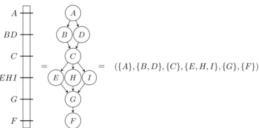
Considering a linear chromosome, the corresponding genetic map should be atotal order on all its markers. However, due to imprecisions, errors or inaccuracies of the techniques, it is usually apartial order on a subset of the markers. This is the case when the relative position of some markers cannot be inferred and they are put at the same position on the map, as illus-trated on the left ofFig 1. We propose to model by a binary relation of order, namely abucket order, maps where several markers are at the same position (Fig 1). A bucket order is a total order onbuckets, each bucket containing elements which are incomparable [3]. Consequently, bucket orders are suitable structures for coding the genetic maps: they allow markers with an uncertain relative order to be gathered in a bucket while preserving the global order informa-tion, namely the bucket sequence. Moreover, even for a single species, we are often faced with several different maps obtained using different input data (e.g. different segregating popula-tion, sequencing techniques etc.) and different techniques or softwares to build a map from those data. The differences come from the subsets of markers positioned on the map or from their order. Recent works [4–6] show that it is possible, by comparing these different maps, to propose a richer and more reliable synthesis than what is obtained by a single approach.
This article focuses on identifying the largest subset of congruent information shared by two maps by identifying theirLongest Common Subsequence (LCS). In the genetic map frame-work, the LCS corresponds to the largest set of collinear markers, i.e. the largest set of markers that appears in the same order in the two compared maps. The LCS hence plays a key role in map comparison, as emphasized by ALLMAP authors: “Collinearity, defined as the arrange-ment of one sequence in the same linear order as another sequence, is one of the most impor-tant criteria in evaluating map concordance and evolutionary relatedness” [6]. Individual maps can be compared based on their correlation coefficients, for marker interval distance and for marker order, based on their LCS using the qualV package [7] as done for comparing switchgrass maps across studies [8,9]. A visual representation of pairwise map collinearity is very helpful and several tools, such as MCScanX [10], VGSC [11] and the genetic map
Fig 1. Simplified genetic map (left) and two different representations: A Directed Acyclic Graph (DAG) (middle) and a bucket order (right). In linkage maps, some markers may have the exact same position on a given map due to
the absence of recombination events between them. In physical maps, this can happen when different genetic markers match at the same place.
comparator [12], provide the so called “dual synteny plot representation”. This representation draws the two maps side by side and traces a line between their common markers. Identifying the LCS allows to highlight map collinearity by using different colors for linking markers that are part of the LCS and those that are not.
The LCS problem is encountered in many contexts, such as file comparison (e.g. unix diff command), computational linguistic analysis (e.g. [13]) or bioinformatics (e.g. sequence com-parison and genome compression [14]) and has thus been extensively studied in computer science [15–17]. Finding a LCS for multiple input sequences has been proved NP-hard [18], while its pairwise counterpart is polynomial and often used in comparative genomics [19–21]. But as far as we know, the LCS problem has never been defined on bucket orders. From here on, we always refer to the pairwise LCS problem. The first step is to precisely define the notion of common subsequence on bucket orders. The adaptation is not so obvious and we propose two definitions relying on the linear extensions of bucket orders; one, calledLongest Common Induced Subsequence (LCIS), being stricter than the other, that is simply called Longest Com-mon Subsequence (LCS). The aim is that LC(I)S captures as much as possible of the consensual information contained in the input maps.
We demonstrate in this paper that we can compute LC(I)S on bucket orders with algo-rithms similar to the classical ones, once an adequate pre-treatment, that we called homogeni-zation, has been performed. The consequence is that the search of the LCS then depends on the number of (homogenized) buckets rather than on the number of markers they contain. This could result in a significant performance improvement for genetic maps where several hundreds of markers can be in total linkage disequilibrium, hence in the same bucket. Homog-enization is a kind ofpartition refinement technique largely used in efficient algorithms on finite automata, string sorting or graphs [22]. Usually, such algorithms run iteratively by split-ting the current partition according to a subset of elements called thepivot. In our case, we homogenize one order/partition by the other order/partition using at the same time all its buckets as pivots. Our procedure leads to a simpler algorithm than [22] while achieving the same time complexity. Faginet al. [23] defined a procedure similar to homogenization on bucket orders but to our knowledge they don’t provide algorithmic detail to produce it nor study its properties.
You will see that the organization of our paper does not follow the standard IMRaD format (Introduction, Methods, Results, and Discussion) as this is not well adapted for a methodologi-cal paper such as this one. In the next section, we present bucket orders and propose two defi-nitions of longest common subsequence for bucket orders (LCS and LCIS). Then, we give details of procedure of homogenization used to allow bucket orders to behave like total orders in terms of time complexity. In the following section, we prove that searching for the LC(I)S of two bucket orders gives the same results as searching for the LC(I)S of their homogenized counterparts. Afterwards, we describe the algorithm which solves the problem, and give a vari-ant to achieve theO(n log(n)) time complexity. Finally, in the last section, we briefly show an application of this work in the framework of dual synteny plots and we use simulated map datasets of various sizes to demonstrate the gain in speed thanks to our optimized LCS routine.
Definitions and notations
In agronomy, marker-assisted selection strongly relies on genetic maps to accelerate breeding programs, see for instance [24]. Genetic maps provide an organization of marker along (frag-ment of) chromosomes. Each marker (SNPs, microsat etc.) is present at most once per genome to be useful for breeding programs. The ordering of those markers can, for instance, be
deduced via the study of their linkage disequilibrium in a segregating population. Linkage dis-equilibrium basically reflects the fact that the value of two markers are not independent. When there is a complete linkage disequilibrium among a set of markers their dependence is total (for any individual of the population, knowing the value of one of those marker is enough to know the value of all other marker of this set). More generally, the higher the dependence between marker values, the closer the markers—since this dependence is related to the number of recombination events that have taken place in the population between those markers (e.g. [24]). Each (fragment) of chromosome of such a map can conveniently be represented by a sequence of bucket of markers, precedence in the sequence reflects precedence on the map while being in the same bucket reflects the fact that we have no clue about the relative position of those markers along this map. As marker are unique, each element/marker appears only once in this bucket sequence. Comparing the marker ordering of one (fragment of) chromo-some proposed by two distinct genetic maps can thus be done by comparing the two equiva-lent bucket orders. Note that though this representation can be extended to store the distance between consecutive buckets of the sequence, we ignore here this information as it is irrelevant for the identification of the LC(I)S.
This section provides a more formal definition of bucket orders introduced above as well as an explicit definition of the LC(I)S on bucket orders. These definitions follow the order classi-fication and notations used in [3].
Abinary relation R on a domain D is a subset of D � D; here we denote x �Ry the fact that
(x, y) 2 R.
A binary relationσ is a strict partial order on D if, and only if, σ is: -irreflexive: 8x 2 D x ⊀sx;
-asymmetric: 8x; y 2 Dx �s y ) y ⊀sx;
-transitive: 8x; y; z 2 D (x �σy and y �σz) ) x �σz.
Two elementsx; y 2 D of a partial order σ are incomparable (x ≹σ y) when neither x �σy
nory �σx.
Definition 1 (Bucket order). A strict partial orderπ on D is a bucket order if, and only if, π isnegatively transitive, i.e. 8x; y; z 2 D (x ⊀πz and z ⊀πy) ) x ⊀πy. It follows that D is
parti-tioned into a sequence ofbuckets B1, . . .,Btso thatx �πy , (x 2 Bi,y 2 Bjandi < j). In a
bucket order, elements are incomparable if, and only if, they belong to the samebucket. We denote by |Bi| the number of elements in bucketBi.
For example,π1= ({k}, {a, b}, {l, c}, {d, e, f}, {i, j}, {g, h}) is a bucket order on the domain
D1¼ fa; b; c; d; e; f ; g; h; i; j; k; lg, which contains 6 buckets (for instance B1= {k}, |B4| = 3),
and wherea ≹p1b while a �p1c. A genetic map can easily be modelled by bucket orders on D,
whereD is the set of its markers.
Do not confuse bucket orders with indeterminate strings (also known as degenerate string) which are strings involving uncertainty and consist of nonempty subsets of letters over an alphabet S [25,26]. In such strings the same character may appear in several subsets while it is not the case in bucket orders.
Atotal order τ is a complete partial order, that is 8x; y 2 D and x 6¼ y, either x �τy or
y �τx. In other words, all τ elements are comparable and τ is a permutation of the elements of
D. Note that a total order can hence be seen as a bucket order B1; . . . ;BjDjwith all its buckets
The definition of Common Subsequences of bucket orders relies obviously on the defini-tion of a Subsequence of a bucket orderπ. We choose to define the latter as a subsequence of any total order compatible withπ, more formally:
Definition 2 (Bucket order subsequence). Asubsequence of a bucket order σ on D is a sequences = (e1,e2, . . .,el) so that, 81 <i < j < l, ei2D and either ei�σejorei ≹s ej. We
denote by subsequence(σ) the set of those subsequences.
Definition 3 (Bucket order Common Subsequence and LCS). Acommon subsequence of two bucket ordersσ1onD1andσ2onD2is a sequences = (e1,e2, . . .,el) of elements
ofD ¼ D1\D2so that: 81 <i < j < l
1. ei�s1ejorei ≹s1 ej i.e.,s 2 subsequence(σ1)
2. andei�s2ejorei ≹s2 ej i.e.,s 2 subsequence(σ2)
The length ofs is its number of elements, that is to say l. A common subsequence of maxi-mum length is called aLongest Common Subsequence (LCS).
Given two bucket ordersσ1andσ2we denote subsequence(σ1,σ2) the set of their
com-mon subsequences. Letπ1= ({k}, {a, b}, {l, c}, {d, e, f}, {i, j}, {g, h}) and π2= ({g, h}, {c, d, e, f},
{m, q}, {r, a}, {b, n}, {o, p, l}) be two bucket orders. The set of the LCS of π1andπ2is {(c, d, e, f),
(c, d, f, e), (c, e, d, f), (c, e, f, d), (c, f, d, e), (c, f, e, d)} and the length of their LCS is 4.
A common subsequence of two bucket ordersσ1andσ2may arbitrarily arrange elements
that are incomparable in both orders (i.e., such thatei ≹s1ejandei ≹s2ej),e.g. elements d, e
andf in LCS of π1andπ2. In the context of genetic map comparison, one consequence is that
an LCS of two maps may order two elements while no input map does. This is the motivation for the following definition, which is stricter than the previous one.
Definition 4 (Bucket order Common Induced Subsequence and LCIS). Acommon induced subsequence of two bucket orders σ1onD1andσ2onD2is a sequences = (e1,e2, . . .,el) of
ele-ments ofD ¼ D1\D2so that:
1. s 2 subsequence(σ1,σ2) and
2. 81 <i < j < l:
(a) eitherei�s1ejandej⊀s2eior (b)ei�s2ejandej⊀s1ei
The length ofs is its number of elements, that is to say l. A common induced subsequence of maximum length is called aLongest Common Induced Subsequence (LCIS).
Note that the ‘and’ parts of the 2ndcondition are implied by the fact thats 2 subsequence (σ1,σ2) and are just useful reminders. Note also that an LCIS cannot contain several elements
located in the same bucket inσ1and in the same bucket inσ2as they are incomparable in the
two orders.
Given two bucket ordersσ1andσ2we will denote as indSubsequence(σ1,σ2) the set of
their induced subsequences. There is only one LCIS ofπ1andπ2: (a, b, l) and it is of length 3.
As far as we know, it is the first time that bucket orders, precise mathematical objects, are used to model genetic maps –including their blurred part. Moreover, we propose a rigorous extension of the classical problem of the LCS on these bucket orders, along with an alternative problem: the LCIS.
Bucket order homogenization
This section introduces a preprocessing step, that we namedhomogenization, which refines two bucket orders so that those refined orders have only buckets that are either identical or
with no common element. This preprocessing is the cornerstone of our efficient solution to find a LC(I)S of two bucket orders.
Definition 5 (Homogenization of two bucket orders). Let s1 ¼ ðB 1 1; . . . ;B 1 k1Þ be a bucket order onD1and s2¼ ðB 2 1; . . . ;B 2
k2Þ be a bucket order onD2. LetD be D1\D2, for each
ele-mente 2 D. Let pos1(e) and pos2(e) denote the positions of the bucket containing e in the
bucket sequenceσ1andσ2respectively.
Thehomogenization of σ1andσ2associates to those orders the homogenized bucket orders
sh
1and sh2respectively, which are both defined onD and so that 8e; e 02D:
• e and e0belong to the samebucket of sh
1(resp. s
h
2) if, and only if, they are in the same bucket
in bothσ1andσ2,i.e., if, and only if, pos1(e) = pos1(e0) andpos2(e) = pos2(e0);
• thebucket of sh
1(resp. s
h
2) containinge precedes the bucket of s
h
1(resp. s
h
2) containinge 0if,
and only if,pos1(e) < pos1(e0) or (pos1(e) = pos1(e0) andpos2(e) < pos2(e0)) (resp.pos2(e) <
pos2(e0) or (pos2(e) = pos2(e0) andpos1(e) < pos1(e0))).
For example, let
π1= ({k}, {a, b}, {l, c}, {d, e, f}, {i, j}, {g, h}) and
π2= ({g, h}, {c, d, e, f}, {m, q}, {r, a}, {b, n}, {o, p, l}).
Their homogenized counterparts are ph
1 ¼ ðfag; fbg; fcg; flg; fd; e; f g; fg; hgÞ and
ph
2 ¼ ðfg; hg; fcg; fd; e; f g; fag; {b}, {l}).
Property 1. Letσ1be a bucket order onD1,σ2be a bucket order onD2and sh1and s
h
2be
their respective homogenized bucket orders, then sh
1and s
h
2have exactly the same buckets but
not necessarily in the same order.
Proof. By contradiction. Let us assume that there are two elementse1;e2 2D ¼ D1\D2
which are in the samebucket of sh
1but in differentbuckets of s
h
2. Sincee1ande2belong to the
same sh
1bucket it follows, by definition, thatpos1(e1) =pos1(e2) andpos2(e1) =pos2(e2). Hence,
e1ande2are also in the same sh2bucket, which contradicts the initial hypothesis and concludes
the proof.
Algorithm 1: HOMOGENIZATION
Data: Two bucket orders π1 and π2 on domains D1 and D2 respectively. Result: ph
1, the homogenized bucket order of π1 with respect to π2. 1 if D1\D2¼ ; then return an empty bucket order;
2 Let B1¼ ðB1 1; . . . ;B 1 jB1jÞ and B 2 ¼ ðB2 1; . . . ;B 2
jB2jÞ be the ordered sequences of
buckets of π1 and π2 respectively.
// 8e 2 D2, get the position of the bucket containing e in B 2
3 e_to_pos2 an empty hash table; 4 for i from 1 to jB2j do
5 foreach e in B2
i do e_to_pos2.insert(key = e, value = i);
// homogenize sequentially all buckets of B1 to build up ph1 6 ph
1 an empty bucket order; 7 for i from 1 to jB1j do
// harvest the position of B1
i elements in π2. 8 Ltemp an empty list;
9 foreach e in B1
i do
10 if e 2 e_to_pos2 then Ltemp.push(e,e_to_pos2.getValue(e)); // sort Ltemp elements (e, pos2) by increasing pos2.
11 LtempSort sort_increasing(Ltemp);
// create a new bucket per set of (now consecutive) elements of B1
i
which are in a same bucket in π2. 12 buck_pos2 LtempSort[1].second;
13 Buck a new empty bucket;
14 for (e, pos2) from LtempSort[1] to LtempSort[|LtempSort|] do 15 if buck_pos2 = pos2 then
16 Buck.add(e);
17 else // new bucket
18 ph
1.push_back(Buck);
19 Buck new Buck(e);
20 buck_pos2 pos2; // handle last bucket 21 ph
1.push_back(Buck); 22 return ph1;
Before presenting our homogenization algorithm (Algorithm 1), we first give a lemma (proof inS1 Proof) that provides a simple way to homogenize a bucket orderπ1with respect to
π2, when elements inπ1buckets are ordered according to their bucket positions inπ2. Lemma 1. Let p1¼ ðB 1 1; . . . ;B 1 k1Þ and p2¼ ðB 2 1; . . . ;B 2
k2Þ be two bucket orders onD1and
D2respectively. LetB 01
i be an ordered restriction ofB
1
i containing only elements ofB
1
i \D2
organized in increasing order according to their position inπ2, then ph1, the homogenized
ver-sion ofπ1with respect toπ2, is obtained fromπ1by splitting each of itsB01i ¼ ðei1; . . . ;eijB01
ij
Þ buckets between two consecutive elementseisandeisþ1if and only ifeisandeisþ1are in different
buckets inπ281 �s � jB01i j 1.
The Algorithm 1 homogenizes one bucket order considering a second bucket order. To get both ph
1and p
h
2it suffices to use the algorithm twice.
Proposition 1 (Algorithm 1 correction). When called with parametersπ1andπ2, the
Algo-rithm 1 returns the homogenization ph
1ofπ1with respect toπ2.
(Proof inS2 Proof)
Proposition 2 (Time complexity of Algorithm 1). The overall complexity of Algorithm 1 is
O(n log(n)) with n ¼ max ðjD1j; jD2jÞ
Proof. The most time consuming operations are:
1. Initialization ofe_to_pos2dictionary:OjD2j �log ðjD2jÞ (L. 4-5);
2. Creation of theLtemp lists: OðjD1j �log ðjD2jÞÞ as each element ofD1is added only once
to aLtemp list and this addition is made in Oð log jD2jÞ due to the interrogation of the
e_to_pos2dictionary (L. 9-10);
3. Sorting of theLtemp lists: at the ithiteration the list contains jB1
ij elements that can be sorted
using Smoothsort [27] inOðjB1
ijlog ðjB
1
ijÞÞ ¼OðjB
1
ijlog ðjD1jÞÞ. The total time complexity
of this loop is thusOðjD1jlog ðjD1jÞÞ (L. 11).
All other instructions are inO(1), thus the overall complexity of Algorithm 1 is:OðjD2j � log ðjD2jÞ þ jD1j � log ðjD2jÞ þ jD1j � log ðjD1jÞÞ ¼Oð max ðjD1j; jD2jÞ�
log ð max ðjD1j; jD2jÞÞ ¼Oðn log ðnÞÞ.
It is easy to see that Algorithm 1 performs two distinct tasks: sorting elements inπ1buckets
according to their bucket positions inπ2and then splitting the buckets ofπ1. The former is
done inO(n log(n)) while the latter is done in O(n), for two bucket orders of n elements. To achieve a linear time complexity for the overall procedure, it is therefore sufficient to provide sorted buckets to Algorithm 1 or to reduce the complexity of the first task. We give inS1 Algo
a linear time variant of Algorithm 1, assuming that bucket orders are composed of pointers to elements of the domain as assumed in [28].
It is already known that bucket order comparisons algorithmically behave like total order comparisons [29] once each bucket order has been refined with respect to the other [23]. Our
contribution is to propose straightforward algorithms to do this refinement. The two versions of our homogenization procedure are easy to implement, rigorously proven and shown to achieve low time complexity:O(n log(n)) and O(n) respectively. For the latter, we were inspired by the first two steps of the preprocessing used for computing distances between par-tial orders [28].
Homogenization preserves the LC(I)S of two bucket orders
Below we show that we can search for the LC(I)S of bucket orders using their homogenized counterparts without losing any solutions.
Theorem 1. Givenπ1a bucket order onD1andπ2a bucket order onD2, the set of the
com-mon subsequences ofπ1andπ2is identical to the set of the common subsequences of their
homogenized counterpart ph
1and ph2.
Proof. subsequence (π1,π2) � subsequence (ph1; p
h
2)
Lets 2 subsequence(ph
1,ph2). Suppose thats =2 subsequence(π1), as a consequence
there are successive elementss[i] and s[i + 1] so that s½i þ 1� �p1s½i�. Hence there exists a
bucketBk3s[i + 1] preceding a bucket Bl3s[i] and pos1(s[i + 1]) < pos1(s[i]) and, by
con-struction,s½i þ 1� �ph
1s½i�, hence a contradiction and s 2 subsequence(π1). We can show in
the same way thats 2 subsequence(π2), therefores 2 subsequence(π1,π2).
subsequence(π1,π2) � subsequence (ph1; ph2)
By contradiction. Lets 2 subsequence(π1,π2). Since all elements ofs are present in both
π1andπ2they also are inD ¼ D1\D2hence in ph1. Suppose thats is not a subsequence of ph1,
it follows that there are two successive elements ofs, s[i] and s[i + 1], so that s½i þ 1� �ph
1s½i�. As
a consequence there should exist in ph
1a bucketBk3s[i + 1] preceding a bucket Bl3s[i] and
either:
• s[i] and s[i + 1] are in the same bucket in both π1andπ2. However in such a case, by
con-structions[i] and s[i + 1] are in the same ph
1bucket, hence a contradiction.
• s[i] and s[i + 1] are in different π1buckets and sinces is a subsequence of π1, it follows that
pos1(s[i]) < pos1(s[i + 1]). As a consequence, s[i] belongs, by construction, to a bucket of ph1
preceding the one containings[i + 1], hence a contradiction.
• s[i] and s[i + 1] are in the same bucket in π1but not inπ2. Sinces is a subsequence of π2,
pos2(s[i]) < pos2(s[i + 1]). As a consequence, s[i] belongs, by construction, to a bucket of ph1
preceding the one containings[i + 1], hence a contradiction.
As all possible cases lead to a contradiction, the initial hypothesis is impossible ands 2 subsequence(ph
1). We can show in the same way thats 2 subsequence(ph2) and therefore
thats is a subsequence of ph
1and p
h
2.
Theorem 2. Givenπ1a bucket order onD1andπ2a bucket order onD2, the set of the
com-mon induced subsequences ofπ1andπ2is identical to the set of the common induced
subse-quences of their homogenized counterpart ph
1and ph2.
Proof. indSubsequence (π1,π2) � indSubsequence (ph1; p
h
2)
Lets 2indSubsequence(π1,π2). Firsts 2 subsequence(ph1; ph2) (Def. 4 and Theorem
1). Second, by Definition 4, 81 <i < j < l: either i) s½i� �p1s½j� or ii) s½i� �p2s½j�. In case i) s[i] is
in a bucket precedings[j] in ph
1. Hences[i] and s[j] satisfy the 2(a) condition required for s to
be in indSubsequence(ph
1; p
h
2). Similarly, in case ii)s[i] is in a bucket preceding s[j] in p
h
2.
Hences[i] and s[j] satisfy the 2(b) condition required for s to be in indSubsequence (ph
indSubsequence (π1,π2) � indSubsequence (ph1; p h 2) Lets 2 indSubsequence(ph 1; p h
2). Firsts 2 subsequence(π1,π2) (Def. 4 and Theorem
1). Second, by Definition 4, 81 <i < j < l: either i) s½i� �ph
1s½j� or ii) s½i� �ph2s½j�. In case i) s[i]
being in a bucket precedings[j] in ph
1implies that eithers½i� �p1s½j� or (s½i� ≹p1s½j� and
s½i� �p2s½j�). In both cases s[i] and s[j] satisfy the 2
ndcondition required fors to be in
indSubsequence(π1,π2). Similarly in case ii)s[i] being in a bucket preceding s[j] in ph2
implies that eithers½i� �p2s½j� or (s½i� ≹p2s½j� and s½i� �p1s½j�). In both cases s[i] and s[j] satisfy
the 2ndcondition required fors to be in indSubsequence(π1,π2).
Theorems 1 and 2 provide a formal proof that searching for the LC(I)S of two bucket orders π1andπ2gives the same result as searching for the LC(I)S of their two homogenized
counter-parts ph
1and p
h
2.
Algorithm for LC(I)S of two bucket orders
Note that the number of markers is potentially decreased by the homogenization procedure and that ph
1and p
h
2have the same (number of) markers and buckets (Property 1). In this
sec-tion we denote by jD1j and jD2j the number of elements ofπ1andπ2respectively; byn the
maximum of those two values; and bynbandnhthe number of buckets and markers contained
in the homogenized orders ph
1and p
h
2. It followsnb�nh�n.
Lemma 2. After homogenization, buckets are either fully identical or share no common
ele-ment (Proof. Direct consequence of Property 1).
Lemma 3. The LCIS of ph
1and p
h
2contain only one element per homogenized bucket (Proof.
Direct consequence of Definition 4).
It follows from these two lemmas 2 properties:
Property 2. Finding a LCIS ofπ1andπ2is finding a LCS of the bucket sequences of ph1
and ph
2.
Property 3. Finding a LCS ofπ1andπ2is finding a Heaviest Common Subsequence (HCS)
of the bucket sequences of ph
1and p
h
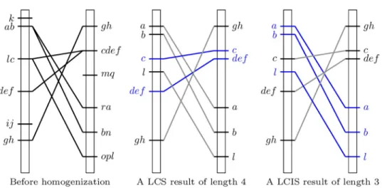
2where each bucket is weighted by its number of elements. Fig 2(left) illustrates the comparison of genetic mapsπ1andπ2, as well as the comparison
of genetic maps from ph
1and ph2(middle and right) in terms of LC(I)S results (in blue). A subset
of non conflicting markers can be seen as a set of non-intersecting edges.
To compute the LC(I)S of two bucket ordersπ1andπ2, we can use the classical quadratic
dynamic programming scheme for LCS/HCS [30] on the two sequences of buckets of the homogenized orders ph
1and ph2. This is what is done in Algorithm 2. The only subtlety is to
manage to recognize identical buckets in constant time. For this, it is sufficient to note that even if the elements of a bucket are incomparable, they are represented in memory by a linear structure. It is then sufficient to choose a total order onD ¼ D1\D2(e.g., the lexicographic
order) and to represent all the buckets ofπ1andπ2in this order. Testing the equality of two
buckets is then equivalent to testing the equality of their first elements (cf. Line 9 of Algorithm 2).
Algorithm 2 begins with the homogenization ofπ1andπ2, assuming their buckets are
ordered using the same total order, and then classically fills the dynamic programming matrix with the lengths of the LCS or LCIS of ph
1and p
h
2prefixes, depending on whether the boolean
induced is false or not. Note that the homogenization (Algorithm 1) does not modify the order of bucket elements if they are already ordered in the same way, so buckets of ph
1and p
h
2are also
ordered according to the same total order as those ofπ1andπ2. It then follows the
Proposition 3. (Algorithm 2 correction). Given two bucket ordersπ1andπ2and a boolean
induced, Algorithm 2 returns a LCS of π1andπ2ifinduced is false, and an LCIS of π1andπ2
otherwise.
Algorithm 2: LC(I)S
Data: Two bucket orders π1 and π2 with bucket elements ordered according to a same total order and a boolean induced
Result: One of the LC(I)S of input orders. // homogenizing the two bucket orders
1 ph1 Homogenization(π1,π2); ph2 Homogenization(π2,π1); 2 Let Bh1¼ ðBh1 1; . . . ;B h1 jBh1jÞ and B h2¼ ðBh2 1; . . . ;B h2
jBh2jÞ be the ordered sequences of buckets of ph
1 and ph2 respectively 3 nb jB
h1j; //jBh1j ¼ jBh2j by Property 1
// filling the matrix L with the LC(I)S lengths of ph
1 and ph2 prefixes 4 L a new matrix of size (nb + 1) × (nb + 1);
5 for i from 0 to nb do 6 L[i, 0] 0; L[0, i] 0; 7 for i from 1 to nb do 8 for j from 1 to nb do 9 if Bh1 i ½1� ¼B h2 j ½1� then 10 if induced then 11 L[i, j] L[i − 1, j − 1] + 1; 12 else 13 L½i; j� L½i 1;j 1� þ jBh1 i j; 14 else
15 L[i, j] max(L[i − 1, j], L[i, j − 1]); // building a LC(I)S of π1 and π2 by backtracking L 16 τ an empty sequence; i nb; j nb; 17 while i > 0 et j > 0 do 18 if Bh1 i ½1� ¼B h2 j ½1� then 19 if induced then 20 t:push frontðBh1 i ½1�Þ 21 else 22 foreach e in Bh1 do
Fig 2. Comparison of two genetic maps before (left) and after (middle and right) homogenization. The blue
elements of the scheme in the middle proposes a consensus without conflict corresponding to an LCS, while on the right they show a consensus without conflict corresponding to the LCIS ofπ1= ({k}, {a, b}, {l, c}, {d, e, f}, {i, j}, {g, h})
andπ2= ({g, h}, {c, d, e, f}, {m, q}, {r, a}, {b, n}, {o, p, l}).
23 τ.push_front(e) 24 i − −; j − −;
25 else if L[i, j − 1] > L[i − 1, j] then
26 j − −;
27 else
28 i − −;
29 return τ;
Proof. The proof is straightforward as Algorithm 2 uses the classical methods [31] to retrieve an HCS of ph
1and p
h
2, giving an LCS ofπ1andπ2(Property 3), wheninduced is false
and an HCS of ph
1and p
h
2, giving an LCIS ofπ1andπ2(Property 2), otherwise.
Time complexity of Algorithm 2 depends on 3 points:
1. Homogenization isO(n) or O(n log(n)) depending whether the linear version of the homogenization algorithm is used or not (Line 1);
2. The filling of the matrix isOðn2
bÞ, withnbthe number of buckets (Lines 4-15);
3. The backtracking procedure isO(nb) for retrieving a LCIS orO(nh) to retrieve a LCS
(Lines 16-28).
The overall time complexity of Algorithm 2, dominated by points 1 and 2, is thus at most Oðn logðnÞ þ n2
bÞ. In the worst case scenario, where all buckets contain only one marker and
all markers are present in bothπ1andπ2,nbequalsn and the complexity is O(n
2
) –just as for the naive solution. In all other cases our solution has a lower time complexity and is faster. The gain in performance increases with the size of the buckets and the number of markers appear-ing in a sappear-ingle input order.
We give inS2 Algoan alternative version of Algorithm 2 that does not need to assume a total order onD nor similar bucket orderings as it includes bucket order preprocessing (done by Algorithm 1 presented in the following section).
The use of the classical dynamic programming approach has several advantages. Building and storing the full dynamic matrix of intermediary common subsequence lengths allows Algorithm 2 not only to get the length of LC(I)S (stored in the last matrix cell), but also to build a LC(I)S using the backtrack procedure. This also allows, with slight adaptation of the back-tracking procedure, to count all the LC(I)S or to return several of them instead of a single one.
To improve time complexity, we can benefit from the LCS algorithmic improvements such as the one of Masek and Paterson [16] that, assuming that the sizes of subsequences are bounded, avoids having to fill the whole dynamic matrix and gives a faster algorithm with O(n log(n) + nblog(nb)) time. Moreover, if one is only interested in getting the length of the
LC(I)S, or getting a sole LC(I)S representative among the possibly numerous ones, a more effi-cient solution to tackle this problem is to rely on the Longest Increasing Subsequence (LIS). A problem that can be solved inO(n log(n)).
In this section we have shown that we can use the classical LCS approach on bucket orders with the same quadratic time complexity. The advantage of considering bucket orders is that the solution is quadratic on the number of homogenized buckets instead of being quadratic in the number of markers within the input maps. When numerous markers are positioned on the same location, or when the compared map have numerous specific markers, this leads to a drastic improvement in speed.
Time complexity improvement using LIS
Once again, to be able to use classical algorithms for the LIS problem we have to carefully pre-treat our bucket orders. We give in this section Algorithm 1 that constructs suitable data
structures to encode the necessary information for the LIS computation (seeFig 3for an exam-ple). Note that this preprocessing can also be used combined with Algorithm 1 to compute LCS (seeFig 4). The necessary information elements are for each bucket of each order: - An identifier (buckets with same identifier are fully identical)
- Its elements
- The number of elements it contains
To test inO(1) whether or not a bucket of ph
1is identical (i.e. contains the same elements as)
a bucket of ph
2, Algorithm 3 relies on aid(.) function that assigns an integer between 1 and
jD1[D2j to each bucket so thatid(Bi) =id(Bj) ,Bi=Bj.
Proposition 4. A unique identifier can be assigned to ph
1and ph2buckets inOðn log ðjD1jÞÞ
and this identifier can be chosen to reflect the bucket position inBh1.
Algorithm 3: LCS-PRE-PROCESS
Data: Two bucket orders π1 and π2 on domains D1 and D2 respectively. Result: Two arrays info ph
1 and info p
h
2 so that info p
h
1½i� (resp info p
h
2½i�) contains: the ith bucket of ph
1 (resp ph2), the integer identifier of this bucket and the number of elements it contains.
1 ph1 Homogenization(π1,π2); ph2 Homogenization(π2,π1); 2 Let Bh1¼ ð Bh1 1; . . . ;B h1 jBh1jÞ and B h2¼ ð Bh2 1; . . . ;B h2
jBh2jÞ be the ordered sequences of buckets of ph
1 and ph2 respectively. 3 e_to_buck_id an empty hash table; 4 nb jB
h1j; //jBh1j ¼ jBh2j by Property 1
// Assign bucket id based on their position in ph1, initiate info p
h
1 5 info ph
1 new info array of size nb + 1;
Fig 3. Example of computation of LCIS using LIS withπ1andπ2. The LIS of the sequence of identifiers from
info ph
2½1�, (6, 3, 5, 1, 2, 4), is (1, 2, 4) and gives the LCIS ofπ1andπ2: (a, b, l).
6 info ph 1½0�:id 1; 7 for i from 1 to nb do 8 info ph 1½i�:bucket B h1 i ; 9 info ph 1½i�:id i; 10 info ph 1½i�:nbElt jB h1 i j; 11 foreach e in Bh1 i do
12 e_to_buck_id.add(key = e, value = buck_id); 13 info ph
2 new info array of size nb + 1;
14 info ph
2½0�:id 2;
// Due to homogenization all elements of a bucket Bh2
i are in the
same Bh1 bucket, use its first element Bh2
i ½1� to get its id
15 for i from 1 to jBh2j do
16 buck id e to buck id:getValueðBh2 i ½1�Þ; 17 info ph 2½buck id�:bucket B h2 i ; 18 info ph
2½buck id�:id buck id; 19 info ph 2½buck id�:nbElt jB h1 2j; 20 return (info ph 1, info ph2);
Proof. The procedure is described in Algorithm 3. The first loop iterates over all buckets of
Bh1, initiatesinfo ph
1and saves, for each element, the identifier of the bucket it belongs to in a
hash table. This is done in timeOðjD1jlog ðjD1jÞÞ. The second loop iterates over all buckets of
Bh2and for each bucket uses its first element to query the hash table containing the bucket
identifier associated to each element. This is done in timeOðjD2jlog ðjD1jÞÞ. Hence the overall
complexity ofOð max ðjD1j; jD2jÞlog ðjD1jÞ, which is quite similar toO(n log(n)).
Once the two data structuresinfo ph
1andinfo p
h
2are computed by the application of
Algo-rithm 3 onπ1andπ2, it follows the 2 properties:
Property 4. Finding a LCIS ofπ1andπ2is finding a LIS of the sequence of bucket
identifi-ers stored ininfo ph
2;
Property 5. Finding a LCS ofπ1andπ2is finding, ininfo ph2, a Heaviest Increasing
Subse-quence (HIS) of the seSubse-quence of bucket identifiers where the elements are weighted by the cor-responding bucket size.
Hence, we can obtain an LC(I)S ofπ1andπ2inO(n log(n) time by using Algorithm 3
fol-lowed by either theO(n log(log(n))) LIS algorithm by [15], as our homogenized orders can be consider as permutations, (for LCIS) or by theO(n log(n)) Jacobson and Vo’s algorithm for HIS [31] (for LCS).
We give inS3 Algoa linear time variant of Algorithm 3, assuming that bucket orders are composed of pointers to elements of the domain.
To conclude the methodological part of this article, we present inFig 4a graph that sums up our whole contribution in term of algorithms on bucket orders.
Application to genetic map visual comparison
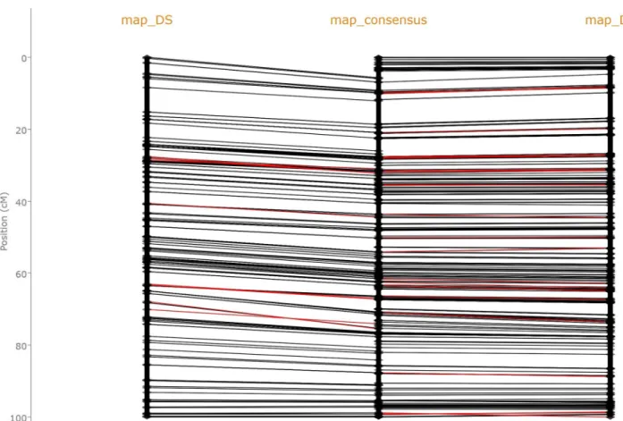
Two high density durum wheat genetic maps, each made of thousands of markers, were obtained thanks to high throughput genotyping of the offsprings of two pairs of progenitors: Dic2xLoyd (map_DL) and Dic2xSilur (map_DS) using specific allelic capture and high throughput sequencing [32]. A practical application of finding LC(I)S is illustrated inFig 5, which is a screenshot of theGenetic Map Comparator [12] (http://www.agap-sunshine.inra.fr/ genmapcomp/) when used to compare those two durum wheat maps together with their con-sensus. This visual representation confirms that the maps are highly congruent. Their discrep-ancies in chromosome 3A, highlighted by the red edges onFig 5, are circumvent to few
regions that could result from small chromosomal rearrangements in those regions between Loyd and Silur progenitors.
The Genetic Map Comparator is an R Shiny application made to facilitate genetic map comparisons. One of the challenges for such a tool is to visually emphasize the collinear mark-ers on the two adjacent maps, as well as the breakpoints. This can be done by identifying (a minimal set of) crossing edges and coloring them differently; which can be done by identifying the minimal subset of markers that should be removed to avoid crossing edges. When consid-ering maps as partial orders, corresponding to Directed Acyclic Graph (DAG), the problem is related to the Minimum Breakpoint Linearization problem, which is known to be NP-hard [33]. The Genetic Map Comparator authors’ tackle this problem by using a brute force heuris-tic to identify congruent markers using the following two-step approach: 1/ for each map a total order is built by tie breaking markers using their position in the other map and, as a last
Fig 4. A graph summarizing algorithmic contributions on bucket orders. Each root to tip path of this graph
provides a pipeline that chains algorithms to obtain the LCS, the LCIS, or both the LCS and LCIS of 2 input bucket ordersπ1andπ2. The framed nodes of this graph represent the computation steps while the other nodes are the input
and/or output of those steps. The algorithms that can be used at each computation step, together with its complexity for this specific task are shown in grey. Note that we count only the time complexity of the specific part of each algorithm. For example, Algorithm 2 calls an algorithm for the Homogenization part, which we don’t count here, as it appears higher on the path. The overall time complexity of a pipeline to get a LCS/LCIS ofπ1andπ2is the sum of the
complexities encountered along the corresponding root to tip path. For example, the time complexity of the pipeline that returns a LCS(π1,π2) by chainingS1andS3Algo and HIS algo [31] (thick arrow path) is O(n) + O(nh) +
O(nhlog(nh)) = O(n log(n)).
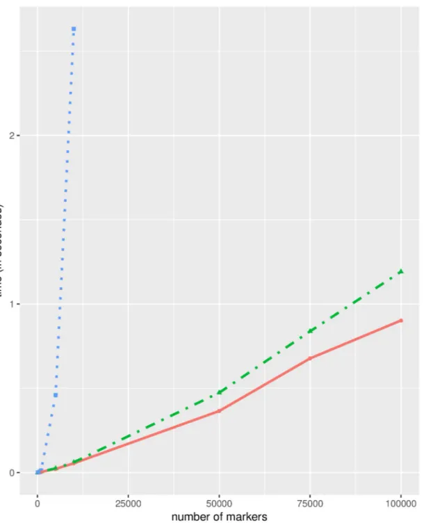
resort, the marker name (a procedure similar to the first step of our homogenization proce-dure) 2/ the LCS of those two fully ordered sequences of markers is computed using the stan-dard LCS algorithm implemented in the qualV R package [7]. Which turns out to be an exact (but computationally non optimal) solution for the LCS problem of the input bucket orders (this is now obvious thanks to the results provided in this paper). A much more efficient solu-tion is to use the bucket map model and dedicated LC(I)S algorithms described in this paper. As the two compared solutions are guaranteed to return an optimal LCS, the solutions pro-posed by the two approaches are equally good and the only difference between these methods is the time they need to return the searched LCS. To emphasize the speed up brought about by our solution, we simulate pairs of bucket orders containing 100, 500, 1000, 5000, 10000, 50000, 75000 and 100000 markers. The first order of each pair is obtained by randomly assigning its n markers to n/10 buckets, while the second order is obtained by swapping 10% of the buckets and moving randomly 10% of the markers (the simulation script is available on LCSLCIS github repository). On the laptop used to conduct the tests (intel i7-6600U, 16Gb RAM), our LC(I)S solution can easily handle datasets of 100,000 markers in seconds whereas the qualV LCS implementation is unable to handle datasets containing 50,000 markers. Both solutions are extremely fast for very small datasets, but the speed difference rapidly increases with the number of markers (Fig 6).
Fig 5. Screenshot of a comparison of three genetic maps of the 3A chromosome of durum wheat displayed by theGenetic Map Comparator. The
map_DS (right) and map_DL (left) were obtained using different durum wheat progenitors; map_consensus (middle) is the consensus of those two maps as proposed by [32]. For this comparison, two LCS have been computed: the LCS of map_DS and map_consensus and the LCS of map_DL and map_consensus. Markers present in two adjacent maps are then connected by black, or red, edges depending on whether they are, or not, part of their LCS.
Moreover our formalization of the problem sheds light on the fact that two equally mean-ingful formulations of this problem exist depending on whether we weight crossing edges by the number of pairs of markers they link (LCS) or not (LCIS) and both problems can be solved efficiently in the special case of bucket orders.
Fig 6. Comparison of computation times in seconds (Y axis) needed to compute LC(I)S for an increasing number of markers (X axis). Three methods
are compared: our bucket dedicated methods to compute 1/ LCS (dashed green line) or 2/ LCIS (plain red line) and 3/ a brute force solution ignoring bucket order specificities and relying on the LCS function of the qualV package (blue dotted line). This latter solution is unable to handle large dataset, and crashes the Rstudio environment when called with the 50000 marker dataset whereas our solutions easily handle much larger datasets in seconds.
Conclusion
In this article, we are interested in the problem of comparing two genetic maps by finding their similarities and their differences. For that, we chose to use their LCS which is their largest set of collinear markers. We proposed a new modeling for genetic maps: bucket orders, a pre-cise mathematical object that is able to encode uncertainties about marker positions in maps, while retaining relative position information. We have stated two simple problems: the classi-cal LCS problem adapted to bucket orders and the LCIS problem that prevents the possible random ordering of markers (non comparable in both input orders) observed in the LCS. For each of these problems, we have proposed algorithms that are simple to program, efficient in computation time and rigorously proven. These algorithmic improvements are especially rele-vant for genetic maps built from SNPs observed in segregating populations where numerous markers are often in total linkage disequilibrium and placed at the exact same position/ bucket along the genetic map. These algorithms are implemented in the R package, named LCSLCIS, ready to replace an already existing slower routine used to accomplish the exact same task. Finally, we have illustrated the effectiveness of our approach by applying it to the visual comparison of genetic maps.
The main contribution of the present work is hence twofold. First it provides a theoretical framework when considering genetic maps as bucket orders including a formal definition of i) the LC(I)S for two bucket orders ii) the homogenization of two bucket orders and iii) proof that the LC(I)S is unchanged by the homogenization procedure. Second, it provides a toolkit of simple though efficient algorithms to compute LC(I)S that can be reused by various genetic map related applications. For instance ALLMAPS [6] orient and order sequence scaffolds by minimizing the sum of LCS distance between the considered scaffold organization and some input genetic maps. The LC(I)S procedure introduced here can thus advantageously replace the one used in ALLMAP to efficiently deal with markers located at the same position. The Genetic Map Comparator also relies on an LCS routine to pinpoint incongruent marker posi-tions in different genetic maps and could also benefit from the optimized solution we pro-posed. Tools which search to build a consensus of several genetic maps, such as MergeMap [34], DAGGER [4] could also benefit from this work. Any genetic map related tool relying on LCS subroutine can safely replace its current LCS subroutine by ours –to do the exact same work but faster– and could thus benefit from a significant speed up while preserving its accu-racy. To widen the fields of application, it would be interesting to use these results to design an efficient heuristic able to efficiently search for a genetic map that is the median of several input maps in so far as the LC(I)S related measurements are concerned. Such a heuristic could be used, for example, to construct the backbone of a consensus map efficiently.
Supporting information
S1 Proof. Proof of Lemma 1.(PDF)
S2 Proof. Proof of Proposition 1.
(PDF)
S1 Algo. Linear homogenization. This algorithm is a linear version of Algorithm 1 assuming
that bucket orders are composed of pointers to elements of the domain. This version is inspired by a trick found in [28] to preprocess bucket orders by relabeling the domainD by the integers from 1 to jDj.
S2 Algo. LC(I)S from LCS-pre-process. Algorithm S2 Algo is an alternative version of
Algo-rithm 1 that does not need to assume a total order onD nor similar bucket orderings as it relies on the preprocess of Algorithm 1 (or its linear version AlgorithmS3 Algo).
(PDF)
S3 Algo. Linear LCS-pre-process. Algorithm S3 Algo is a linear version of Algorithm 1
assuming that bucket orders are composed of pointers to elements of the domain, using the same trick as AlgorithmS1 Algo.
(PDF)
Author Contributions
Conceptualization: Lisa De Matte´o, Vincent Ranwez, Sèverine Be´rard.
Formal analysis: Vincent Ranwez, Sèverine Be´rard.
Funding acquisition: Sèverine Be´rard.
Investigation: Lisa De Matte´o.
Methodology: Vincent Ranwez, Sèverine Be´rard.
Software: Lisa De Matte´o, Yan Holtz, Vincent Ranwez. Supervision: Vincent Ranwez, Sèverine Be´rard.
Validation: Yan Holtz, Vincent Ranwez, Sèverine Be´rard.
Visualization: Yan Holtz.
Writing – original draft: Lisa De Matte´o, Vincent Ranwez, Sèverine Be´rard.
Writing – review & editing: Vincent Ranwez, Sèverine Be´rard.
References
1. Sturtevant AH. The linear arrangement of six sex-linked factors in Drosophila, as shown by their mode of association. Journal of Experimental Zoology. 1913; 14:43–59.https://doi.org/10.1002/jez. 1400140104
2. Cone KC, Coe EH. In: Genetic Mapping and Maps. New York, NY: Springer New York; 2009. p. 507–522.
3. Brandenburg F, Gleißner A, Hofmeier A. The nearest neighbor Spearman footrule distance for bucket, interval, and partial orders. J Comb Optim. 2013; 26(2):310–332. https://doi.org/10.1007/s10878-012-9467-x
4. Endelman JB. New algorithm improves fine structure of the barley consensus SNP map. BMC Geno-mics. 2011; 12(1):407.https://doi.org/10.1186/1471-2164-12-407PMID:21831315
5. Endelman JB, Plomion C. LPmerge: an R package for merging genetic maps by linear programming. Bioinformatics. 2014; 30(11):1623–1624.https://doi.org/10.1093/bioinformatics/btu091PMID: 24532720
6. Tang H, Zhang X, Miao C, Zhang J, Ming R, Schnable JC, et al. ALLMAPS: robust scaffold ordering based on multiple maps. Genome Biology. 2015; 16(1):3.https://doi.org/10.1186/s13059-014-0573-1 PMID:25583564
7. Jachner S, van den Boogaart KG, Petzoldt T. Statistical Methods for the Qualitative Assessment of Dynamic Models with Time Delay (R Package qualV). Journal of Statistical Software. 2007; 22(8):1–30. https://doi.org/10.18637/jss.v022.i08
8. Li G, Serba D, Saha MC, Bouton J, Lanzatella CL, Tobias C. Genetic Linkage Mapping and Transmis-sion Ratio Distortion in a Three-Generation Four-Founder Population of Panicum virgatum (L.). 2014; 4:5 913–5923.
9. Fiedler J, Lanzatella C, Okada M, Jenkins J, Schmutz J, Tobias C. High-Density Single Nucleotide Poly-morphism Linkage Maps of Lowland Switchgrass using Genotyping-by-Sequencing. 2015; 8.
10. Wang Y, Tang H, Debarry JD, Tan X, Li J, Wang X, et al. MCScanX: A toolkit for detection and evolu-tionary analysis of gene synteny and collinearity. 2012; 40:e49.
11. Xu Y, Bi C, G, S, Dai X, Yin T, et al. VGSC: A Web-Based Vector Graph Toolkit of Genome Synteny and Collinearity. 2016; 2016:8.
12. Holtz Y, David J, Ranwez V. The genetic map comparator: a user-friendly application to display and compare genetic maps. Bioinformatics. 2017; 33(9):1387–1388.https://doi.org/10.1093/bioinformatics/ btw816PMID:28453680
13. Silfverberg M, Liu L, Hulden M. A Computational Model for the Linguistic Notion of Morphological Para-digm. In: COLING; 2018. p. 1615–1626.
14. Beal R, Afrin T, Farheen A, Adjeroh D. A new algorithm for “the LCS problem” with application in com-pressing genome resequencing data. In: 2015 IEEE International Conference on Bioinformatics and Biomedicine (BIBM); 2015. p. 69–74.
15. Hunt JW, Szymanski TG. A Fast Algorithm for Computing Longest Subsequences. Commun ACM. 1977; 20(5):350–353.https://doi.org/10.1145/359581.359603
16. Masek WJ, Paterson M. A Faster Algorithm Computing String Edit Distances. J Comput Syst Sci. 1980; 20(1):18–31.https://doi.org/10.1016/0022-0000(80)90002-1
17. Apostolico A. Improving the Worst-Case Performance of the Hunt-Szymanski Strategy for the Longest Common Subsequence of Two Strings. Inf Process Lett. 1986; 23(2):63–69.https://doi.org/10.1016/ 0020-0190(86)90044-X
18. Maier D. The Complexity of Some Problems on Subsequences and Supersequences. J ACM. 1978; 25(2):322–336.https://doi.org/10.1145/322063.322075
19. Delcher AL, Kasif S, Fleischmann RD, Peterson J, White O, Salzberg SL. Alignment of whole genomes. Nucleic Acids Research. 1999; 27(11):2369.https://doi.org/10.1093/nar/27.11.2369PMID:10325427
20. Vialette S, Bonizzoni P, Dondi R, Della Vedova G, Fertin G, Rizzi R. Exemplar Longest Common Sub-sequence. IEEE/ACM Transactions on Computational Biology and Bioinformatics. 2007; 4:535–543. https://doi.org/10.1109/TCBB.2007.1066PMID:17975265
21. Beal R, Afrin T, Farheen A, Adjeroh D. A new algorithm for “the LCS problem” with application in com-pressing genome resequencing data. BMC Genomics. 2016; 17(4):544.https://doi.org/10.1186/ s12864-016-2793-0PMID:27556803
22. Habib M, Paul C, Viennot L. Partition Refinement Techniques: An Interesting Algorithmic Tool Kit. Int J Found Comput Sci. 1999; 10(2):147–170.https://doi.org/10.1142/S0129054199000125
23. Fagin R, Kumar R, Mahdian M, Sivakumar D, Vee E. Comparing Partial Rankings. SIAM J Discrete Math. 2006; 20(3):628–648.https://doi.org/10.1137/05063088X
24. Wen W, He Z, Gao F, Liu J, Jin H, Zhai S, et al. A High-Density Consensus Map of Common Wheat Inte-grating Four Mapping Populations Scanned by the 90K SNP Array. Front Plant Sci. 2017; 8:1389. https://doi.org/10.3389/fpls.2017.01389PMID:28848588
25. Holub J, Smyth WF. Algorithms on indeterminate strings. 2003; p. 36–45.
26. Daykin JW, Watson B. Indeterminate String Factorizations and Degenerate Text Transformations. Mathematics in Computer Science. 2017; 11(2):209–218.https://doi.org/10.1007/s11786-016-0285-x
27. Dijkstra EW. Smoothsort, an Alternative for Sorting In Situ. Sci Comput Program. 1982; 1(3):223–233. https://doi.org/10.1016/0167-6423(82)90016-8
28. Bansal MS, Ferna´ndez-Baca D. Computing distances between partial rankings. Inf Process Lett. 2009; 109(4):238–241.https://doi.org/10.1016/j.ipl.2008.10.010
29. Brandenburg FJ, Gleißner A. Ranking chain sum orders. Theor Comput Sci. 2016; 636:66–76.https:// doi.org/10.1016/j.tcs.2016.05.026
30. Wagner RA, Fischer MJ. The String-to-String Correction Problem. J ACM. 1974; 21(1):168–173. https://doi.org/10.1145/321796.321811
31. Jacobson G, Vo K. Heaviest Increasing/Common Subsequence Problems. In: Combinatorial Pattern Matching, Third Annual Symposium, CPM 92, Tucson, Arizona, USA, April 29—May 1, 1992, Proceed-ings; 1992. p. 52–66.
32. Holtz Y, Ardisson M, Ranwez V, Besnard A, Leroy P, Poux G, et al. Genotyping by Sequencing Using Specific Allelic Capture to Build a High-Density Genetic Map of Durum Wheat. Plos One. 2016; 11(5). https://doi.org/10.1371/journal.pone.0154609
33. Bulteau L, Fertin G, Rusu I. Revisiting the Minimum Breakpoint Linearization Problem. Theor Comput Sci. 2013; 494:122–133.https://doi.org/10.1016/j.tcs.2012.12.026
34. Wu Y, Close TJ, Lonardi S. Accurate Construction of Consensus Genetic Maps via Integer Linear Pro-gramming. IEEE/ACM Transactions on Computational Biology and Bioinformatics. 2011; 8(2):381–394. https://doi.org/10.1109/TCBB.2010.35PMID:20479505