Source Separation in Chemical Analysis : Recent Achievements and Perspectives

HAL Id: hal-00985017

https://hal.archives-ouvertes.fr/hal-00985017

Submitted on 29 Apr 2014

HAL is a multi-disciplinary open access archive for the deposit and dissemination of sci-entific research documents, whether they are pub-lished or not. The documents may come from teaching and research institutions in France or abroad, or from public or private research centers.

L’archive ouverte pluridisciplinaire HAL, est destinée au dépôt et à la diffusion de documents scientifiques de niveau recherche, publiés ou non, émanant des établissements d’enseignement et de recherche français ou étrangers, des laboratoires publics ou privés.

Achievements and Perspectives

Leonardo Tomazeli Duarte, Saïd Moussaoui, Christian Jutten

To cite this version:

Leonardo Tomazeli Duarte, Saïd Moussaoui, Christian Jutten. Source Separation in Chemical Analy-sis : Recent Achievements and Perspectives. IEEE Signal Processing Magazine, Institute of Electrical and Electronics Engineers, 2014, 31 (3), pp.135-146. �10.1109/MSP.2013.2296099�. �hal-00985017�

Source Separation in Chemical Analysis:

Recent Achievements and Perspectives

Jutten, Fellow, IEEE

I. INTRODUCTION

Since its origins in the mid-1980s, the field of blind source separation (BSS) has attracted considerable attention within the signal processing community. One of the main reasons for such popularity is the existence of many problems that can be addressed in a BSS framework. Two noteworthy examples of applications can be found in audio and biomedical signal processing, for which a number of efficient solutions are now available. Additionally, there are relevant BSS problems in other domains but for which less effort has been put on. In this article, we deal with one of these fields, namely the field of analytical chemistry (AC), whose goal of is to identify or quantify, or both, chemical components present in a given analyte, i.e. the sample under analysis. As recently discussed in [1], several tasks in AC keep some relationship to the broad classes of detection and estimation problems typically found in signal processing.

Source separation is one of the most relevant estimation problems found in chemistry. Indeed, dealing with mixtures is paramount in different kinds of chemical analysis. For instance, there are some cases where the analyte is a chemical mixture of different components, e.g., in the analysis of rocks and heterogeneous materials through spectroscopy. Moreover, a mixing process can also take place even when the components are not chemically mixed. For instance, in ionic analysis of liquid samples, the ions are not chemically connected, but, due to the lack of selectivity of the chemical sensors, the acquired responses may be influenced by ions that are not the desired ones. Finally, there are some situations where the pure components cannot be isolated chemically since they appear only in the presence of other components. In this case, BSS may provide these components that cannot be retrieved otherwise.

In AC, there is a trend that advocates acquiring data through sensor arrays or by other instruments that are able to exploit diversity, which is essential in the application of source separation methods. Especially,

This work has been partially funded by the European project ERC-2012-AdG-320684-CHESS. L. T. Duarte would like to thank FAPESP (S˜ao Paulo, Brazil) for funding his research.

Chemometrics [2], a sub field of AC, aims at extracting the relevant information from the multivariate signals provided by the chemical measurement sensor. Chemometrics is an established domain of research based on different backgrounds (physics, statistics, computer science, etc.). Several approaches that are now popular in signal processing arose in chemometrics — a typical example is a problem introduced in the 1970’s known as multivariate curve resolution (MCR) [3], which bears strong resemblance to non-negative matrix factorization (NMF) [4].

Classically, the available methods in chemometrics for dealing with mixtures work in a supervised fashion, thus requiring a set of training samples. The application of supervised methods in this context has been proving successful in tasks such as odor and taste automatic recognition systems (electronic noses and tongues, respectively). However, despite this success, this approach suffers from, at least, two important practical problems. Firstly, the acquisition of training samples is usually a cost and time-demanding task. Secondly, due to the drift in the response of chemical sensors, which is usually caused by aging and variation of the acquisition conditions (temperature, pH, etc.), the calibration procedure must be performed before each new chemical analysis. Due to these limitations, there is a growing interest in solutions in which the calibration stage may be eliminated or, at least, simplified. This can be achieved by methods, like source separation or multi-way data analysis, able to exploit the measurement diversity for discovering latent variables. The goal in considering these approaches is to ultimately have chemical sensing systems that work in a plug-and-measure fashion, which may pave the way for devices operating in more challenging situations — for example, a calibration-free system would be quite helpful in the context of invasive physiological monitoring by means of miniaturized sensors.

Given the panorama described above, our aim is to shed some light on the use of BSS in chemical analysis. In this context, we firstly provide a brief overview on source separation (Section II), with particular attention to the classes of linear and nonlinear mixing models (Sections III and IV, respectively). Then, (in Section V), we will give some conclusions and focus on challenging aspects that are found in chemical analysis. Although dealing with a relatively new field of applications, this article is not an exhaustive survey of source separation methods and algorithms, since there are solutions originated in closely related domains (e.g. remote sensing and hyperspectral imaging) that suit well several problems found in chemical analysis. Moreover, we do not discuss the supervised source separation methods, which are basically multivariate regression techniques, that one can find in chemometrics.

II. SOURCESEPARATION IN CHEMICAL ANALYSIS

Let us briefly recall the problem of source separation. The observed signals, which are represented by the vector x(n) = [x1(n), x2(n), . . . , xM(n)]T, are given by:

x(n) = A(s(n)), (1)

where A(·) represents the operator associated to the mixing process, and the vector s(n) = [s1(n), . . . , sN(n)]T denotes the source signals. The goal in source separation is to provide a good estimation of s(n). In a blind (or unsupervised) context, one has access neither to training points, i.e. a set of pairs (xi(n), si(n)), nor to the mixing system A(·). Therefore, based only on observations x(n), solving Equation (1) for s(n) becomes an ill-posed inverse problem whose handling requires further information ([5], chapters 7, 10, 11 and 13). For instance, a possible approach is to exploit measurement diversities such as time-frequency representations of nonstationary signals (see for example [5], chapter 11).

1) Source assumptions: Source separation can be solved with independent component analysis (ICA) [6, 7], in which the sources are modeled as mutually independent random variables. Under some mild conditions, including the non-gaussianity of the sources, the application of ICA ensures a correct retrieval of the sources. It is also possible to achieve source separation by exploiting properties other than statistical independence, e.g. sparsity or non-negativity [5]. Moreover, one can separate sources that are only mutually uncorrelated provided that additional temporal priors on the source signals hold, e.g., nonstationary or temporally correlated sources. This is very important in chemical applications since there are some cases in which the source independence assumption fails. For instance, when a chemical reaction takes place, the components exhibit dependency since either they are made of the same chemical elements or their concentrations vary according to stoichiometric coefficients, which stands for the coefficients in a balanced chemical equation.

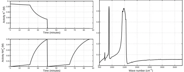
In chemical analysis, the sources present some features that can be exploited when developing a novel separation method. For instance, in ionic activity analysis (the effective concentration of an ion), the source signals correspond to time-series associated with the activities of each ion within the solution under analysis. Therefore, a first remarkable aspect is that the sources here are always non-negative, since there is no physical meaning in having a negative concentration. A second prior information is the fact that source signals are smooth, i.e. successive samples are temporally correlated. Indeed, concentrations usually present slow variations of amplitude along time. In order to illustrate these features, we show in Figure 1(a) an example of sources related to the concentrations of potassium and ammonium ions and

acquired in two different experiments. These data are publicly available at the ISEA dataset [8]. 0 10 20 30 40 50 60 70 80 90 0 0.02 0.04 0.06 0.08 0.1 Time (minutes) Activity K + (M) 0 10 20 30 40 50 60 70 80 90 0 0.01 0.02 0.03 0.04 0.05 Time (minutes) Activity NH 4 + (M)

(a) Ionic activities (in molar concentration) of potassium and ammonium. Note that the time scale is in minutes, and the signals were obtained from two different experiments.

500 1000 1500 2000 2500 3000 3500 0 0.1 0.2 0.3 0.4 0.5 Wave number (cm−1)

(b) Infrared reflectance of calcite.

Fig. 1. Examples of sources in chemical analysis.

Another category of chemical source signals are those obtained in optical spectroscopy (Raman, Infrared, etc.). Again, there are some valuable information that can be exploited: (1) the sources are again non-negative, since they correspond to absorption, reflectance or diffusion spectra, (2) there exist many libraries containing the spectra of different chemical components. This information can be used to adapt BSS algorithms based on sparse representation over a huge dictionary whose atoms are the pure component spectra. However, it would be difficult to use a reference library since the component spectra may present some variability in actual experiments depending on parameters such as temperature or pH condition. In Figure 1(b), an example of spectral source (infrared reflectance of calcite) is provided.

2) Mixing models: A lot of effort was undertaken to develop methods tailored to linear and instan-taneous mixing systems in which the number of sources is equal to the number of mixtures (N = M ). Practically, this assumption implies that the number of sources is known, which is often a tricky issue. In this case, the operatorA(·) is given by a square matrix A ∈ RN ×N_{. Moreover, there are many works} that deal with the convolutive case, in which each entry of the mixing matrix corresponds to a linear filter. Finally, there is an important topic in BSS where the aim is to set up separation methods in the case of nonlinear mixing models. In this context, one must bypass many difficulties that do not arise in the linear case. For instance, ICA does not ensure separation in a general nonlinear context, that is, retrieving independent components is not enough to reconstruct the actual sources. As a consequence,

some researchers have been considering constrained classes of nonlinear model for which ICA is still valid. For instance, ICA-based solutions ensure source separation in an important class of constrained models known as post-nonlinear (PNL) models ([5], chapter 14). In chemical mixture analysis, one can find in the literature works on both linear and nonlinear mixing models. In the sequel, we provide an (non-exhaustive) overview of source separation problems arising in each situation.

III. LINEAR MODELS

Measurement techniques such as optical spectroscopy and/or chromatography are frequently used in chemical analysis to extract relevant information related to the chemical composition of an heterogeneous material (identify the components and assess their relative abundance [9]). The data processing corre-sponds to a source separation problem where the linear instantaneous mixture model holds with relatively small concentrations of the components in absorption spectroscopy, thanks to the Beer-Lamber law [10]. In such model, each measured spectrum xi(λ) is a linear combination of the component spectra sj(λ), and the mixing coefficients aij are related to the abundances of each component:

xi(λ) = N ∑ j=1

aijsj(λ). (2)

In practice, M spectra (i.e., i = 1 . . . M in (2)) are measured for different chemical conditions and L values of a spectral variable (frequency, wavelength or wavenumber) λ. Figure 2(b) illustrates three absorption spectra resulting from the linear mixing of two spectral sources, shown in Figure 2(a). By considering a matrix notation for Equation (2) and a noise term, the measured spectra can be stored in the rows of the data matrix X ∈ RM ×L_{, that can thus be factorized according to X = AS + E. The} pure component spectra are identified as the sources (rows of matrix S ∈ RN ×L_{) and the abundance} fraction of each component are the elements of the mixing matrix A ∈ RM ×N_{. Matrix E ∈ R}M ×L represents measurement errors and any deviation from the linear mixing model. In the chemical analysis community, the problem of estimating S and A knowing only matrix X is termed by Multivariate Curve

Resolution, Spectral Mixture Analysis and Factor Analysis while in signal and image processing field this problem is called Source Separation and Spectral Unmixing.

In order to develop a linear spectral mixture separation method, an objective function must be obtained by formulating some assumptions on the sought component spectra (the sources) and on their abundances (the mixing coefficients). Then, one must define a mathematical algorithm to optimize this objective function. The main information in spectral mixture data analysis is the non-negativity of both the pure component spectra and abundances. However, even with a linear mixing model, only accounting for

4000 600 800 1000 1200 1400 0.005 0.01 4000 600 800 1000 1200 1400 0.005 0.01

spectral variable spectral variable

(a) Pure component spectra

400 600 800 1000 1200 1400 −0.001 0 0.004 0.008 400 600 800 1000 1200 1400 −0.001 0 0.004 0.008 400 600 800 1000 1200 1400 −0.001 0 0.004 0.008

spectral variable spectral variable spectral variable

(b) Mixture spectra

Fig. 2. Example of three absorption spectra resulting from the linear mixing of two components with abundance fractions (75%, 25%), (60%, 40%) and (30%, 70%) respectively.

these constraints does not lead to a unique solution [3]. Additional constraints or assumptions are thus used to select a particular (and meaningful) solution among the feasible ones [11]. The existing methods differ on the way the constraints and the additional assumptions are formulated and how the separation is performed. A short overview of the different approaches is firstly given in this section and an example illustrates the application of one of these techniques to the separation problem.

A. Independent Component Analysis

As mentioned before, since BSS is an ill-posed inverse problem, prior knowledge and/or additional assumptions should be used to get a unique and correct solution. Principal component analysis (PCA) [12] assumes that the signals to be reconstructed are mutually uncorrelated but this orthogonality constraint does not ensure the non-negativity of the solution. A more constraining statistical assumption used for source separation is the mutual independence of the sources, leading to the ICA concept [5], for which many algorithms have been developed (see [5]). If the sought source signals are mutually statistically independent, they can be separated successfully by ICA methods and their non-negativity will be ensured implicitly (at least, only few negative values appear in the estimates) as reported in [13], where a

second-order blind identification (SOBI) algorithm [14] was applied to the analysis of nuclear magnetic resonance (NMR) data. But, when the source signals are not mutually independent or when their mutual independence is not observed due to the finite and small number of samples, the non-negativity information should be considered. In [15], Plumbley showed that it is possible to incorporate jointly non-negativity and mutual independence of the sources (See also in [5], chapter 13). This method yields a correct solution providing the condition of well-grounded sources (that is sources having non-vanishing probability distributions around zero) is fulfilled.

B. Multivariate Curve Resolution

This approach, proposed by Lawton and Sylvestre [3], termed by multivariate curve resolution, firstly decomposes the data matrix, using Principal Component Analysis (PCA), X = U V . Then, a linear transformation T is calculated in order to transform the principal components V and their weight matrix U into non-negative estimates of pure spectra S = T V and mixing coefficients A = U T−1, respectively. Since accounting for non-negativity alone does not ensure the uniqueness of the solution, this approach leads to several possible values of matrix T which provide the set of admissible (feasible) solutions [3]. In order to reduce this set Sasaki et al. [16] suggests to add further constraints, in addition to the non-negativity, and proposes to search a linear transformation T by minimizing a two-term criterion, in which a first part penalizes negative estimates of the pure spectra and mixing coefficients, and the second part uses an entropic cost function to make the estimated spectra smoother and mutually independent. The resulting optimization is given by:

min T  ∥ min(S, 0)∥2_F + ∥ min(A, 0)∥2_F + β L ∑ n=1 N ∑ j=1 sj(n) log sj(n)  ,

where ∥ · ∥F stands for the Frobenius norm and β is a regularization parameter that allows to adjust the trade-off between the two parts. The optimization of the whole objective function is performed by using the Nelder-Mead algorithm. However, this method may converge to local or spurious minima since this criterion in non-convex and the criterion shape highly depends on the regularization parameters that should be specified manually. This method was revisited in [17] where a simulated annealing optimization algorithm is used. In the signal processing community, the algebraic approach for ICA is very similar to that of Lawton-Sylvestre but it is based on the statistical independence of the source signals (pure spectra). To get mutually independent signals, the transformation matrix is reduced to a unitary rotation matrix by minimizing a contrast function ([5], chapter 3). Assuming the independence of the sources leads to a unique solution but it does not guarantee its non-negativity.

C. Non-negative Matrix Factorization

This approach performs a constrained least squares estimation of S and A ( ˆS, ˆA) = argmin

S_,A

||X − AS||2F.

This (non-convex) optimization problem can be solved using alternating least square (ALS) with alternate exact solving [11] or multiplicative [4] alternate update methods. At each iteration k, ALS algorithms minimize alternatively the above criterion with respect to S, keeping A fixed, or to A, keeping S fixed, with non-negativity constraints [18] on S and A. It leads to solve the following optimization problems ˆ S(k)= argmin S ||X − ˆA(k−1)S||2_F s.t. S > 0 (3) ˆ A(k)= argmin A ||X − ˆAS(k)||2_F s.t. A > 0. (4)

Multiplicative methods update iteratively the estimates of the sources and the mixing coefficients using a particular multiplicative learning rule that ensures the non-negativity [4]. However since the criterion is non-convex, NMF algorithms do not lead a unqiue solution, unless in some particular conditions [19]. Therefore, the NMF results highly depend on the algorithm initialization. Several contributions proposed to initialize the algorithm by the results obtained with an unconstrained decomposition method such as PCA, factor analysis algorithms, or using pure variable detection methods such as simple-to-use interactive

self modeling mixture analysis (SIMPLISMA) [20] and orthogonal projection approach (OPA) [21]. In [13], for NMR spectroscopy, it has been shown that ICA methods can be used successfully for the initialization of the ALS approach. However, each initialization leads to a local minimum of the criterion and none of these methods has proven to outperform the others since the result of each method highly depends on the data at hand.

Similarly to the case of curve resolution methods, additional constraints such as sum-to-one (also called closure or full additivity) and unimodality (i.e. presence of only one maximum in each column of matrix A) may be added to reduce the set of admissible solutions [22]. The sum-to-one constraint corresponds to assuming that the sum of the elements of each row of matrix A is equal to one (or to a known constant). This is the case for instance in reaction-based systems, where a mass balance equation is obeyed by the concentration profiles of the species present in the system. See for instance [23]1. Another constraint that

1_{However, adding this constraint can alter the separation performance if the number of sources is not correctly selected or if}

reduces the set of admissible solution is the local rank or selectivity [22] which refers to the fact that for certain rows or columns of the data matrix, some mixing coefficients are known to be non-zero while other coefficients are known to have zero values.

There are other constraints that can be taken into account through a penalized least squares estimation approach. This idea is used in positive matrix factorization (PMF) [25] (this work was historically the first one dealing with spectral mixture analysis as a matrix factorization problem under positivity constraints) where the criterion to minimize is

min S_,A  ||X − AS||2_F + α||A||2_F + β||S||2_F − γ L ∑ n=1 N ∑ j=1 log sj(n) − δ M ∑ i=1 N ∑ j=1 log aij  . (5)

The hyperparametersγ and δ control the strength of the logarithmic barrier function that prevents negative values of the source samples and mixing coefficients. Hyperparameters α and β allows to adjust the weight of the quadratic regularization criteria. Contrarily to the constrained least squares methods, the PMF approach leads to an unconstrained optimization problem.

It is also possible to consider the sparsity constraint through a penalized least squares approach. Such an idea gives rise to non-negative sparse coding (NNSC) [26], which searches for minimizing the following cost function min S_,A(||X − AS|| 2 F + β||S||1 ) s.t. A > 0 and S > 0. (6)

This approach was applied by [27] for the analysis of magnetic resonance chemical shift imaging data. There are other alternative approaches for reducing the set of admissible solutions, see for instance [28] and [29].

D. Bayesian Approaches

The formulation of source separation using Bayesian estimation theory is reported in details in ([5], chapter 12). Its first application to the separation of spectral mixture data has been proposed in [30]. The spectral mixture separation in a Bayesian framework consist in describing the statistical properties of the measurement noise and assigning parametric a priori distributions p(S|θ) and p(A|θ) on the pure com-ponent spectra and abundances, respectively. These distribution are defined with some hyperparameters represented by θ. A multivariate Gaussian distribution is generally used to model the noise statistics, which yields the likelihood

where N (µ, Σ) stands for the Gaussian distribution with mean µ and covariance matrix Σ. This matrix reduces to σ2I_L when the noise samples are assumed to be independent and identically distributed. In order to account for the non-negativity and the sparsity of the component spectra, a Gamma distribution model was used in [30], while a truncated Gaussian distribution or a Dirichlet distribution can be used to encode the sum-to-one constraint on the mixing coefficients [31].

The key point of the Bayesian approach is to apply Bayes’ theorem to express the a posteriori density,

p(S, A|X, θ, Σ) = p(X|A, S, θ, Σ) p(A|θ) p(S|θ, Σ)/p(X), (7)

from which a statistical inference is conducted to perform the separation. This distribution combines explicitly the available assumptions on the pure component spectra and their abundances with the infor-mation coming from the measured data. The inference of the unknown quantities can be conducted by minimizing J(S, A) = − log p(S, A|X, θ) or calculating empirical posterior means of S and A after drawing samples fromp(S, A|X, θ) using Monte Carlo Markov Chain (MCMC) methods (See [30, 31] for details). The first approach is equivalent to minimizing a criterion similar to (6) with regularization criteria R(A) and R(S) linked to the prior distributions according to R(A) = − log p(A|θ) and R(S) = − log p(S|θ), while the second approach allows to infer all the weighting parameters at the price of a significant increase of the computation time. The Bayesian method was successfully applied for the analysis of Hyperspectral data in [32] and chemical reaction monitoring [33].

E. Geometrical Methods

Geometrical methods are based on the empirical distribution (geometrically speaking, the scatter plot) of the mixture data. Since these data result from a non-negative mixing of non-negative data, the scatter plot of the mixed data is contained in the simplicial cone generated by the columns of the mixing matrix [19]. Figure 3 illustrates three examples of mixture data distribution for different types of sources. It can be noted that in the case of sparse sources, each row of S has a dominant peak at some location (column number) where other rows have zero elements, then the problem of finding the columns of the mixing matrix A reduces to the identification of the edges of a similicial cone, edges where the data are concentrated 3(b). In the case of sum-to-one mixing, the mixture data will be distributed on a simplex whose vertices correspond to mixture data containing only one component. component. Thus, each vertice is associated with a column of the mixing matrix A. In [34], efficient algorithms are designed for data where the sources are not well grounded and the mixing matrix does not satisfy the sum-to-one or the

pure pixel assumptions. This method can also handle noisy data and was applied to Positron emission tomography (PET) imaging and mass spectroscopy.

0 0.5 1 1.5 0 0.5 1 1.5 0 0.5 1 1.5 x1 (a) x₂ x 3 0 0.5 1 1.5 0 0.5 1 1.5 0 0.5 1 1.5 x1 (b) x₂ x 3 0 0.5 1 1.5 0 0.5 1 1.5 0 0.5 1 1.5 x1 (c) x₂ x 3

Fig. 3. Illustration of the simplicial cone and the empirical distribution of the mixture data for three types of non-negative sources : (a) uniform well grounded sources, (b) sparse sources and (c) uniform sources with sum-to-one mixing constraint.

In chemical imaging spectrometry and remote sensing by hyperspectral imaging [35, 36], the spectral mixture analysis is often handled using a two step procedure: the pure spectra estimation and the abundance fraction assessment, respectively. In the first step, the pure component of the mixture are identified by using an Endmember Extraction Algorithm (EEA). See for instance [37] for a recent performance comparison and discussion on EEAs. The most popular EEAs is the N-FINDR algorithm. N-FINDR estimates the pure component spectra by identifying the largest simplex whose vertices are taken from the convex hull of the data. Another popular and faster alternative is the (Vertex Component

Analysis-VCA) method which has been proposed in [38]. It consists in iteratively estimating the vertices of the simplex without calculating the convex hull. A common assumption in VCA and N-FINDR is the existence of pure pixels (pixels composed of a single component) in the observed data. Alternatively, the

Minimum Volume Transform (MVT) finds the smallest simplex that contains all the pixels [39, 40]. The second step of the spectral unmixing can use various strategies such as those based on constrained least squares estimation [41].

F. Tensorial methods

Most of the above methods simply exploit one type of diversity: it leads to a 2-way array of data, easily represented by a matrix. Above examples consider 2-way arrays based on space and time (mixtures of signals), or space and frequency (spectral mixtures) dimensions. But in many chemical experiments,

one or more additional diversities can be considered, leading to a 3-way (or more generally a multi-way) array of data, which can be represented by a tensor. As an example, in fluorescence spectroscopy, the (measured) fluorescence intensity dependents on 3 variables: the fluorescence emission spectrum, the absorbance spectrum and the relative concentration of the components. Of course, tensorial decompo-sition is not restricted to fluorescence, and other applications include time resolved spectroscopy [42], multidimentional NMR [43] or polarized Raman spectroscopy [44].

Historically, PARAFAC or canonical polyadic decomposition (CPD) - inspired from early works on factor analysis in psychometrics - has been intensively studied in chemometrics from 90’s and popularized by R. Bro [18]. Currently, many theoretical contributions and applications are addressing CPD decomposition of 3-way arrays. More details and references of tensorial methods and an application in fluorescence spectroscopy are provided, respectively, in the articles [45] and [46], found in the present special issue.

G. Application Example

Calcium carbonate is a chemical material used for a large variety of applications such as filler for plastics or paper. Depending on operating conditions, Calcium carbonate crystallizes as Calcite, Aragonite or Vaterite. The formation of Calcium carbonate by mixing two solutions containing respectively Calcium and Carbonate ions takes place in two steps. The first step is the precipitation one, which is very fast and provides a mixture of Calcium carbonate polymorphs. The second step (a slow process) represents the phase transformation from the unstable polymorphs to the stable one (Calcite). The physical properties of the crystallised product depend largely on the polymorphic composition, so it is necessary to quantify these polymorphs when they are mixed. The main purpose of this application is to study the relation of polymorphs and temperature and to explore favorable conditions for Calcite formation.

Calcium chloride and Sodium carbonate separately dissolved in Sodium chloride solutions of the same concentration were rapidly mixed to precipitate Calcium carbonate. A sample was collected 2 minutes after the beginning of the experiment to determine the polymorphic composition at the end of the precipitation step. Raman spectra of this sample have been measured for various temperatures ranging between 20oC and 70oC to determine the influence of temperature on the polymorphs precipitation. Moreover for each temperature, Raman spectra were collected at regular time intervals for monitoring the phase transformation. Finally, a total of M = 37 spectra (each one obtained for a given temperature and phase transformation time) of L = 477 wavelengths are obtained. Details on the experiment can be found in [33]. Figure 4(a) shows Six spectra measured at the beginning the phase transformation step.

50 100 150 200 250 300 350 400 450 0 2000 4000 6000 8000 10000 12000 14000 16000 18000 20000 T = 20 oC T = 30 oC T = 40 oC T = 50 oC T = 60 oC T = 70 oC wavenumber (cm−1)

Raman intensity (a.u)

100 150 200 250 300 350 0 2000 4000 Intensity (a.u) wavenumber (cm−1) Vaterite 0 5000 10000 Intensity (a.u) Aragonite 0 6000 12000 Intensity (a.u) Calcite estimated reference estimated reference estimated reference (a) (b) 20 30 40 50 60 70 0 10 20 30 40 50 60 70 80 90 100 Temperature (oC) abundance (%) Calcite Aragonite Vaterite 0 1 2 3 4 5 6 7 8 0 10 20 30 40 50 60 70 80 90 100 time (h) abundance (%) Calcite Aragonite Vaterite (c) (d)

Fig. 4. Separation of Raman spectra of calcium carbonate: mixture data and separation results. (a) Collected mixture spectra at 2 minutes after the beginning of the phase transformation for different temperature values. (b) Comparison between the estimated sources (continuous) and the reference spectra (dashed) of the three components. (c) Abundances of the three components at the beginning of the phase transformation for different temperature values. (d) Temporal evolution of the three component

abundances at T=40o

C.

Figure 4(b) shows the estimated sources using a Bayesian separation approach with a Gamma distribu-tion prior on the sources and a Dirichlet distribudistribu-tion as prior on the mixing coefficients [30, 31]. From the spectroscopic point of view and according to the locations of the vibrational peaks, the identification of the three components is easy. The evolution of the concentration profile versus the temperature is shown in Figure 4(c). It can be deduced that pure Vaterite is observed at 20oC and a quite pure aragonite is obtained at 60oC . However, between 20oC and 60oC ternary mixtures are observed. The abundance of calcite is maximal at 40oC which is in agreement with results reported in the literature. Let us now

consider the phase transformation evolution at this temperature value. The concentration profile versus precipitation time at 40oC is shown in Figure 4(d). At the beginning of the phase transformation (2 minutes), the ternary mixture is composed of 50% vaterite, 35% aragonite and 15% calcite. Then, after 2 hours, the Vaterite is transformed to Aragonite and Calcite. Finally, after 7 hours, Vaterite and Aragonite are almost totally transformed to Calcite. So, aging time promotes the formation of Calcite.

IV. NONLINEAR MODELS

Although linear mixing models provide a satisfactory first-order approximation of the measurement process in several applications, there are some cases in which a nonlinear model is mandatory. Indeed, exploiting the physical theory behind the measurement transducer allows to increase the amount of information that can be extracted from the data. For example, the sensitive membrane of potentiometric sensors such as ion-selective electrodes (ISEs) or ion-selective field effect transistors (ISFETs) can be described by the classical Nernst equation [47], which establishes a logarithmic relation between ionic activity and the membrane potential. In this section we shall discuss how source separation methods can be set to deal with nonlinear mixing models, paying special attention to the illustrative example of ISE arrays. Afterward, some considerations on other types of sensors are made.

ISEs, which are the most used chemical sensors in industry, are simple devices for measuring ionic activity. A well know example of ISE is the glass electrode, which is used for measuring the pH of a given solution. Besides, one can find ISEs tailored to different ions such as ammonium, potassium and sodium. These devices have been intensively used, for instance, in food and soil inspection, clinical analysis and water quality monitoring. One of the reasons that explains the success of ISEs in such applications is the simplicity of this approach. Indeed, ISE-based analyses do not require sophisticated laboratory equipments and procedures and, thus, can be carried out in the field if necessary. Although attractive, potential electrodes such as ISEs and ISFETs suffer from an important drawback: they are not selective, that is, the generated potential depends on a given target ion but also on other undesirable ions, which are called interfering ions [47]. There are some situations in which this interfering process is so weak that it can be neglected. However, this phenomenon may become important when the target ion and the interfering ones have similar physical and/or chemical properties. A possible solution to eliminate this interference effect is to consider the diversity provided by an ISE array using a source separation approach.

The interference in ISE can be modeled through an empirical extension of the Nernst equation called the Nicolsky-Eisenman (NE) equation [47]. According to this model, the response of the i-th sensor

(dedicated to measure the i-th ion) within the array is given by xi(n) = ei+ dilog  si(n) + ∑ j,j̸=i aijsj(n)zi/zj  , (8)

wheredi andei are constants that depend on some physical parameters,zi andsi(n) denote, the valence and the activity of thei-th ion, respectively. The non-negative parameters aij, the selectivity coefficients, explain the influence (interference) of the j-th ion on the i-th sensor; n stands for the temporal index.

There are some pairs of ions for which high values of selectivity coefficients are observed. When the valences of the ions are different, the model (8) becomes difficult to deal with because a nonlinearity (power term) appears inside the logarithm term [48]. However, when the valences are equal, which is the most common situation, Equation (8) becomes a special nonlinear (NL) model known as post-nonlinear (PNL) model [49]. Indeed, in PNL systems, there is a linear mixing stage followed by a set of component-wise nonlinear function, which in the case of ISE arrays correspond to logarithms. As mentioned before, an interesting property of PNL models is that, under conditions that are close to those required in the linear case [5], the application of ICA leads to source separation.

A. Nonlinear Independent Component Analysis

For equal valences, when the number of mixtures and sources is the same, the mixing process described in (8) can be counterbalanced by a separating system in which each estimated source is given by

yk(n) = M ∑

i=1

wkiexp(fi+ hixi(n)), for k = 1, . . . , N (9) where wki, fi andhi are unknown parameters that must be adjusted andM the number of sensors and N the number of target ions— actually, the parameters fi only introduce a scale ambiguity, which is usual in BSS, and, therefore, can be fixed a priori to a given value.

As in the linear case, the adjustment of PNL separating models can be performed by means of ICA, but some care must be taken while developing the separation algorithm. For instance, one must resort to stronger independence measures such as the mutual information. The adjustment of the separating system is thus carried out by the following optimization problem

min wki,hi

I(y1(n), . . . , yN(n)), (10)

where I(y1, . . . , yN) denotes the mutual information between the estimated signals y(n). There are several algorithms for solving (10), where main difficulties are related to the estimation of the mutual information and to the existence of spurious local minima in this cost function. In [50], for instance,

the optimization problem expressed in (10) was tackled by a bio-inspired optimization method that is robust to convergence to local minima and that does not require the calculation of the derivatives of (10). Moreover, [50] adopts a mutual information estimator based on order statistics.

In order to illustrate the application to a real situation of the ICA method [50], we considered an experiment where the data was acquired by an array composed of a sodium and a potassium ISE (two mixtures). Therefore, there are two mixtures and two sources (the activities of potassium and sodium). Data acquisition was achieved via a flow-injection analysis system, which usually increases the stability and the sensitivity of the array. In Figure 5(a), the actual sources are depicted. As a result of the low-selectivity of each sensor within the array, the acquired signals correspond to nonlinear mixtures of the sources, which is illustrated in Figure 5(b). After solving the problem (10), the retrieved sources are shown in Figure 5(c). Despite the reduced number of samples (41 points), the ICA technique was able to provide signals that are good approximations of the original sources. A more detailed description of this experiment is provided in [51].

B. Bayesian Approach

Bayesian source separation can also be applied in the context of ISE arrays. Actually, differently from ICA, whose basis lies in the independence assumption, the Bayesian approach does not introduce a measure of independence but it searches a solution allowing to jointly explain the data according to the mixing model and fulfill some prior knowledge. Similarly to the linear case (see Equation (7)), the posterior distribution in the nonlinear case is given by

p(s, A, g|x) = p(x|A, s, g)p(A)p(s)p(g)/p(x), (11)

where the vector g includes the parameters associated with the logarithmic functions (see Equation (8)). As in the linear case, the inference step can be done based on a set of samples drawn from the posterior distribution via MCMC methods. The main difficulty when dealing with nonlinear models using MCMC methods is the need to draw samples from distributions for which classical sampling method may be inefficient. In [49], by relying on lognormal prior distributions on p(s), limited support gaussian densities on p(g), we showed the relevance of accounting for the the non-negativity constraint and introducing auxiliary variables to handle the sampling difficulties.

C. Exploiting other prior information

In addition to the non-negativity of the sources, other prior information can be considered when devel-oping nonlinear source separation methods. For example, in [52], a method exploiting the assumption that

0 5 10 15 20 25 30 35 40 45 0 0.002 0.004 0.006 0.008 0.01 Time Activity Na + (M) 0 5 10 15 20 25 30 35 40 45 0 0.02 0.04 0.06 0.08 0.1 Time Activity K + (M)

(a) Sources: activities of sodium and potassium.

0 5 10 15 20 25 30 35 40 45 0 50 100 150 200 250 Time Na +−ISE (mV) 0 5 10 15 20 25 30 35 40 45 0 50 100 150 200 250 Time K +−ISE (mV) (b) Array response. 0 5 10 15 20 25 30 35 40 45 0 1 2 3 4 Time Estimated source 1 0 5 10 15 20 25 30 35 40 45 0 0.5 1 1.5 2 2.5 3 3.5 Time Estimated source 2 (c) Retrieved sources.

Fig. 5. Experiment with data acquired by an array composed of a sodium and a potassium ISE.

the sources are bandlimited is proposed to compensate the nonlinear stage of PNL systems. The advantage brought by this approach is that, once the nonlinear component-wise functions are counterbalanced, the resulting separation problem becomes linear and, therefore, can be dealt with by means of linear BSS methods. In the context of ISE arrays, assuming bandlimited sources is realistic since the signals of interest have a spectral content concentrated on low-frequency bands. The approach proposed in [52] was applied in the analysis of the ions ammonium and potassium, leading to a good estimation of the sensors’ nonlinearities.

Another prior information that can be considered is the existence of silent periods of a given ion, i.e., time windows in which the concentration of a given ion is approximately zero. Interestingly, this scenario is close to that of found in speech separation and can be interpreted as a sparsity-based approach. In [48],

a method that uses this prior was proposed to estimate the parameters di of (8) in the case where the valences of the ions are different. In this situation, as can be noted in Equation (8), the mixing model is much more complex than PNL model, and, thus, estimating the nonlinearities at first usually simplifies the problem.

D. Linear-quadratic mixing model

In addition to the complex model (8) considered in the context of ISE arrays for analyzing ions with different valences, there is another relevant class of models that arises in chemical analysis: the linear-quadratic (LQ) model ([5], chapter 14). An interesting aspect of the LQ mixture is that it can be seen as linear mixture of dependent sources. Such a feature simplifies the derivation of separation algorithms in this case. According to Clifford-Touma equation [53], the mixing process that takes place in the analysis of two gases by using a tin oxide gas sensor can be described by a LQ model. Moreover, LQ models also arise in the context of hyperspectral imaging, especially when there are multiple reflexions caused by the presence of buildings or trees [36]. This is an interesting problem since hyperspectral imaging is closely-related to the above-mentioned problems of separating spectra. Such a model is also considered in fluorescence spectroscopy of highly concentrated solution, involving a screen effect, and a possible method for solving this problem is proposed in [54].

V. CONCLUSIONS AND FURTHER CHALLENGES

In this article, we aimed at presenting an overview on how source separation methods can be applied in chemical analysis. We briefly discussed some kinds of chemical data, and presented several approaches that can be applied. A typical characteristic of chemical data is the existence of prior information on the sources and the mixing process. These priors have motivated researchers working on the subject to consider alternatives to the framework of ICA, thus showing that, besides being an exciting field of application to classical BSS methods, chemical analysis may also be inspiring environment for novel BSS paradigms. Another interesting aspect of this relatively new field of applications is related to the challenges that are found when developing separation methods, e.g. nonlinear mixtures and dependent sources.

Despite the current advances achieved in source separation for chemical data, there are still many issues that must be tackled.

1) Mixing models: A first important point concerns the mixing models that should be adopted. Indeed, transducer physics gives realistic mixing models whose processing in a raw version or even after some

simplifications will provide very challenging signal processing problems. Moreover, most of the models give a static description, that is, we assume that the mixtures follow an instantaneous model. Therefore, if a dynamical mixing model were available, it would be possible to take advantage of the sensor’s dynamics to obtain better separation results. This could be achieved by considering convolutive models.

2) Noise and measurement process modeling: Another difficult aspect that must be handled in chemical analysis is the existence of noise and other complex phenomena. In ISEs, for instance, since there is nonlinear elements in the transducer stage, there may be a strong noise amplification during the separation process — one can show that a separation method based on inversion leads to a multiplicative noise model [49]. Moreover, in the context of spectral unmizing, finding realistic noise models for non-negative sources is still an open issue. Finally, when dealing with chemical sensors one may find hysteresis, which is a nonlinear and dynamical phenomenon that is very difficult to model.

3) Source number: the source number is one of the oldest questions in signal analysis and remains of huge interest for the application of source separation methods to real applications. In the linear mixing model, additive noise and mutually uncorrelated sources, it is generally addressed by a subspace analysis approach. However, the theory behind such analysis breaks down when dealing with either nonlinear mixing models or non-negative sources. For instance, by considering non-negativity in the linear mixing model the source number corresponds to the non-negative rank which is different from the classical matrix rank. Indeed, when dealing with mixture data related some chemical reaction monitoring, the number of sources will be known in advance.

4) Enhancing the data acquisition setup: the performances of any signal processing method will highly depend on how much the data fulfill the method hypotheses. For instance, the application of NMF will be more efficient when the sources are well grounded, when there is some pure pixels in the spectral image and, more generally, when the uniqueness conditions are respected. It would be therefore useful to pay attention on how to design the measurement setup in such a way to meet, at best, theses conditions or how to introduce additional measurement modalities to make the mixture analysis problem more tractable. In that respect, chemists play a fundamental role here especially in data acquisition. There is a great number of different acquisition techniques, even for the same kind of analysis, and many properties, such as temperature, pH, pressure, humidity, that when correctly controlled by a chemist, may lead to a good diversity within the acquired data. Therefore, in order to further advance in the application of source separation in chemistry, the collaboration between researchers in the fields of analytical chemistry and signal processing should be reinforced, even more than before.

REFERENCES

[1] L. Duval, L. T. Duarte, and C. Jutten, “An overview of signal processing issues in chemical sensing,” Proceedings of IEEE

ICASSP 2013, pp. 8742–9746, 2013.

[2] J. N. Miller and J. C. Miller, Statistics and Chemometrics for Analytical Chemistry. Prentice-Hall, 2005.

[3] W. H. Lawton and E. Sylvestre, “Self-modeling curve resolution,” Technometrics, vol. 13, pp. 617–633, 1971.

[4] D. Lee and H. Seung, “Learning the parts of objects by non–negative matrix factorization,” Nature, vol. 401, pp. 788–791, 1999.

[5] P. Comon and C. Jutten, Eds., Handbook of blind source separation: independent component analysis and applications. Academic Press, 2010.

[6] C. Jutten and J. H´erault, “Blind separation of sources, part i: An adaptive algorithm based on neuromimetic architecture,”

Signal processing, vol. 24, no. 1, pp. 1–10, 1991.

[7] P. Comon, “Independent component analysis, a new concept?” Signal Processing, vol. 36, no. 3, pp. 287–314, 1994. [8] L. Duarte, C. Jutten, P. Temple-Boyer, A. Benyahia, and J. Launay, “A dataset for the design of smart ion-selective electrode

arrays for quantitative analysis,” IEEE Sensors Journal, vol. 10, no. 12, pp. 1891–1892, 2010.

[9] E. Malinowski, Factor Analysis in Chemistry, 3rd ed. John Willey & Sons, 2000.

[10] H. Pfeiffer and H. Liebhafsky, “The origins of Beer’s law,” Journal of Chemical Education, vol. 28, p. 123, 1951. [11] R. Tauler, A. Izquierdo-Ridorsa, and E. Casassas, “Simultaneous analysis of several spectroscopic titrations with

self-modelling curve resolution,” Chemometrics and Intelligent Laboratory Systems, vol. 18, no. 3, pp. 293–300, 1993. [12] H. Hotelling, “Analysis of a complex of statistical variables into principal components,” Journal of Education and

Psychology, vol. 24, pp. 417–441, 1933.

[13] D. Nuzillard and J.-M. Nuzillard, “Application of blind source separation to 1-D and 2-D Nuclear Magnetic Resonance spectroscopy,” IEEE Signal Processing Letters, vol. 5, no. 8, pp. 209–211, 1998.

[14] A. Belouchrani, K. Abed-Meraim, J.-F. Cardoso, and E. Moulines, “A blind source separation technique using second-order statistics,” IEEE Transactions on Signal Processing, vol. 45, no. 2, pp. 434–444, Feb. 1997.

[15] M. Plumbley, “Algorithms for non–negative independent component analysis,” IEEE Transactions on Neural Networks, vol. 14, no. 3, pp. 534–543, 2003.

[16] K. Sasaki, S. Kawata, and S. Minami, “Constrained nonlinear method for estimating component spectra from multicom-ponent mixtures,” Applied Optics, vol. 22, no. 22, pp. 3599–3606, 1983.

[17] E. Widjaja and M. Garland, “Pure component spectral reconstruction from mixture data using SVD, global entropy minimization, and simulated annealing. numerical investigations of admissible objective functions using a synthetic 7-species data set,” Journal of Computational Chemistry, vol. 23, no. 9, pp. 911–919, 2003.

[18] R. Bro, “PARAFAC. tutorial and applications,” Chemometrics and intelligent laboratory systems, vol. 38, pp. 149–171, 1997.

[19] D. Donoho and V. Stodden, “When does non-negative matrix factorization give a correct decomposition into parts?” in

Advances in Neural Information Processing Systems (NIPS’2003), Cambridge, United States, 2003.

[20] W. Windig and J. Guilment, “Interactive self-modeling mixture analysis,” Analytical Chemistry, vol. 63, pp. 1425–1432, 1991.

[21] F. C. Sanchez, J. Toft, B. van den Bogaert, and D. L. Massart, “Orthogonal projection approach applied to peak purity assessment,” Analytical Chemistry, vol. 68, pp. 79–85, 1996.

[22] R. Tauler, “Calculation of maximum and minimum band boundaries of feasible solutions for species profiles obtained by multivariate curve resolution,” Journal of Chemometrics, vol. 15, no. 8, pp. 627–646, 2001.

[23] A. de Juan, Y. V. Heyden, R. Tauler, and D. Massart, “Assessment of new constraints applied to the alternating least squares method,” Analytica Chimica Acta, vol. 346, no. 3, pp. 307–318, 1997.

[24] E. Chouzenoux, M. Legendre, S. Moussaoui, and J. Idier, “Fast constrained least squares spectral unmixing using primal-dual interior-point optimization,” IEEE Journal of Selected Topics in Applied Earth Observations and Remote Sensing, vol. PP, no. 99, pp. 1–11, 2014.

[25] P. Paatero and U. Tapper, “Positive matrix factorization: a nonnegative factor model with optimal utilization of error estimates of data values,” Environmetrics, vol. 5, pp. 111–126, 1994.

[26] P. O. Hoyer, “Non-negative matrix factorization with sparseness constraints,” Journal of Machine Learning Research, vol. 5, pp. 1457–1469, 2004.

[27] P. Sajda, S.Du, T. Brown, R. Stoyanova, D. Shungu, X. Mao, and L. Parra, “Nonnegative matrix factorization for rapid recovery of constituent spectra in magnetic resonance chemical shift imaging of the brain,” IEEE Transactions on Medical

Imaging, vol. 23, no. 12, pp. 1453–1465, 2004.

[28] A. de Juan, S. Navea, J. Diewok, and R. Tauler, “Local rank exploratory analysis of evolving rank-deficient systems,”

Chemometrics and intelligent laboratory systems, vol. 70, no. 1, pp. 11–21, 2004.

[29] L. Miao and H. Qi, “Endmember extraction from highly mixed data using minimum volume constrained nonnegative matrix factorization,” IEEE Transactions on Geoscience and Remote Sensing, vol. 45, no. 3, pp. 765–777, 2007. [30] S. Moussaoui, D. Brie, A. Mohammad-Djafari, and C. Carteret, “Separation of non-negative mixture of non-negative sources

using a Bayesian approach and MCMC sampling,” IEEE Transactions on Signal Processing, vol. 54, pp. 4133–4145, 2006. [31] N. Dobigeon, J.-Y. Tourneret, and C.-I. Chang, “Semi-supervised linear spectral unmixing using a hierarchical Bayesian

model for hyperspectral imagery,” IEEE Transactions on Signal Processing, vol. 56, no. 7, pp. 2684–2695, 2008. [32] S. Moussaoui, H. Hauksd´ottir, F. Schmidt, C. Jutten, J. Chanussot, D. Brie, S. Dout´e, and J. Benediktsson, “On the

decomposition of Mars hyperspectral data by ICA and Bayesian positive source separation,” Neurocomputing, vol. 71, no. 10-12, pp. 2194–2208, June 2008.

[33] C. Carteret, A. Dandeu, S. Moussaoui, H. Muhr, B. Humbert, and E. Plasari, “Polymorphism studied by lattice phonon Raman spectroscopy and statistical mixture analysis method,” Crystal Growth & Designr, vol. 9, pp. 807–812, 2009. [34] W. S. B. Ouedraogo, A. Souloumiac, M. Jaidane, and C. Jutten, “Simplicial cone shrinking algorithm for unmixing

nonnegative sources,” in Proc. of ICASSP, 2012, pp. 2405–2048.

[35] C.-I. Chang, Hyperspectral Data Exploitation. Wiley Interscience, 2007.

[36] J. M. Bioucas-Dias, A. Plaza, N. Dobigeon, M. Parente, D. Qian, P. Gader, and J. Chanussot, “Hyperspectral unmixing overview: Geometrical, statistical, and sparse regression-based approaches,” IEEE Journal of Selected Topics in Applied

Earth Observations and Remote Sensing, vol. 5, no. 2, pp. 354–379, April 2012.

[37] A. Plaza, P. Martinez, R. Perez, and J. Plaza, “A quantitative and comparative analysis of endmember extraction algorithms from hyperspectral data,” IEEE Transactions on Geoscience and Remote Sensing, vol. 42, no. 3, pp. 650–663, March 2004. [38] J. M. P. Nascimento and J. M. Bioucas-Dias, “Vertex component analysis: a fast algorithm to unmix hyperspectral data,”

IEEE Transactions on Geoscience and Remote Sensing, vol. 43, no. 4, pp. 898 – 910, April 2005.

[39] M. D. Craig, “Minimum-volume transforms for remotely sensed data,” IEEE Transactions on Geoscience and Remote

[40] L. Miao and H. Qi, “Endmember extraction from highly mixed data using minimum volume constrained nonnegative matrix factorization,” IEEE Transactions on Geoscience and Remote Sensing, vol. 45, no. 3, pp. 765–777, Mar. 2007. [41] S. Moussaoui, E. Chouzenoux, and J. Idier, “Primal-dual interior point optimization for penalized least squares estimation

of abundance maps in hyperspectral imaging,” in Proceedings of the IEEE WHISPERS’12, Shanghai, China, June 2012. [42] A. Niazi, J. Ghasemi, and A. Yazdanipour, “Parafac decomposition of three-way kinetic-spectrophotometric spectral matrices

based on phosphomolymbdenum blue complex chemistry for nitrite determination in water and meat samples,” Analytical

letters, vol. 38, no. 14, pp. 2377–2392, 2005.

[43] M. Nilsson, A. Botana, and G. Morris, “T1-diffusion-ordered spectroscopy: Nuclear magnetic resonance mixture analysis using parallel factor analysis,” Analytical Chemistry, vol. 81, no. 19, pp. 8119–8125, 2009.

[44] S. Miron, M. Dossot, C. Carteret, S. Margueron, and D. Brie, “Joint processing of the parallel and crossed polarized raman spectra and uniqueness in blind nonnegative source separation,” Chemometrics and Intelligent Laboratory Systems,, vol. 105, pp. 7–18, 2011.

[45] G. Zhou, A. Cichocki, Q. Zhao, and S. Xie, “Algorithms for nonnegative matrix and tensor factorizations of large-scale and multi-block data,” IEEE Signal Processing Magazine, 2014, in this special issue.

[46] P. Comon and G. Ottaviani, “Tensor decompositions: a brief survey,” IEEE Signal Processing Magazine, 2014, in this special issue.

[47] P. Gr¨undler, Chemical sensors: an introduction for scientists and engineers. Springer, 2007.

[48] L. T. Duarte and C. Jutten, “A nonlinear source separation approach to the Nicolsky-Eisenman model,” in Proceedings of

the 16th European Signal Processing Conference, EUSIPCO 2008, 2008.

[49] L. T. Duarte, C. Jutten, and S. Moussaoui, “A Bayesian nonlinear source separation method for smart ion-selective electrode arrays,” IEEE Sensors Journal, vol. 9, no. 12, pp. 1763–1771, 2009.

[50] L. T. Duarte, R. Suyama, R. R. F. Attux, F. J. V. Zuben, and J. M. T. Romano, “Blind source separation of post-nonlinear mixtures using evolutionary computation and order statistics,” in Independent Component Analysis and Blind

Signal Separation, ser. Lecture Notes in Computer Science. Springer Berlin Heidelberg, 2006, vol. 3889, pp. 66–73. [51] L. T. Duarte, J. M. T. Romano, C. Jutten, K. Y. Chumbimuni-Torres, and L. T. Kubota, “Application of blind source

separation methods to ion-selective electrode arrays in flow-injection analysis,” submitted paper.

[52] L. T. Duarte, R. Suyama, B. Rivet, R. Attux, J. M. T. Romano, and C. Jutten, “Blind compensation of nonlinear distortions: Application to source separation of post-nonlinear mixtures,” IEEE Transactions on Signal Processing, vol. 60, no. 11, pp. 5832–5844, 2012.

[53] N. Yamazoe and K. Shimanoe, “Theory of power laws for semiconductor gas sensors,” Sensons and Actuators B, vol. 128, pp. 566–573, 2008.

[54] X. Luciani, S. Mounier, R. Redon, and A. Bois, “A simple correction method of inner filter effects affecting feem and its application to the parafac decomposition,” Chemometrics and Intelligent Laboratory Systems, vol. 96, no. 2, pp. 227–238, 2009.