• Aucun résultat trouvé

Horizontal shear instabilities in rotating stellar radiation zones

N/A
N/A
Protected

Academic year: 2021

Partager "Horizontal shear instabilities in rotating stellar radiation zones"

Copied!
14
0
0

Texte intégral

(1)

HAL Id: cea-02513759

https://hal-cea.archives-ouvertes.fr/cea-02513759

Submitted on 20 Mar 2020

HAL is a multi-disciplinary open access

archive for the deposit and dissemination of

sci-entific research documents, whether they are

pub-lished or not. The documents may come from

teaching and research institutions in France or

abroad, or from public or private research centers.

L’archive ouverte pluridisciplinaire HAL, est

destinée au dépôt et à la diffusion de documents

scientifiques de niveau recherche, publiés ou non,

émanant des établissements d’enseignement et de

recherche français ou étrangers, des laboratoires

publics ou privés.

Horizontal shear instabilities in rotating stellar radiation

zones

J. Park, V. Prat, S. Mathis

To cite this version:

J. Park, V. Prat, S. Mathis. Horizontal shear instabilities in rotating stellar radiation zones: I.

Inflectional and inertial instabilities and the effects of thermal diffusion. Astronomy and Astrophysics

- A&A, EDP Sciences, 2020, 635, pp.A133. �10.1051/0004-6361/201936863�. �cea-02513759�

(2)

https://doi.org/10.1051/0004-6361/201936863 c J. Park et al. 2020

Astronomy

&

Astrophysics

Horizontal shear instabilities in rotating stellar radiation zones

I. Inflectional and inertial instabilities and the effects of thermal diffusion

J. Park, V. Prat, and S. Mathis

AIM, CEA, CNRS, Université Paris-Saclay, Université Paris Diderot, Sorbonne Paris Cité, 91191 Gif-sur-Yvette, France e-mail: junho.park@cea.fr

Received 7 October 2019/ Accepted 4 February 2020

ABSTRACT

Context.Rotational mixing transports angular momentum and chemical elements in stellar radiative zones. It is one of the key pro-cesses for modern stellar evolution. In the past two decades, an emphasis has been placed on the turbulent transport induced by the vertical shear instability. However, instabilities arising from horizontal shear and the strength of the anisotropic turbulent transport that they may trigger remain relatively unexplored. The weakest point of this hydrodynamical theory of rotational mixing is the as-sumption that anisotropic turbulent transport is stronger in horizontal directions than in the vertical one.

Aims.This paper investigates the combined effects of stable stratification, rotation, and thermal diffusion on the horizontal shear

instabilities that are obtained and discussed in the context of stellar radiative zones.

Methods. The eigenvalue problem describing linear instabilities of a flow with a hyperbolic-tangent horizontal shear profile was solved numerically for a wide range of parameters. When possible, the Wentzel–Kramers–Brillouin–Jeffreys (WKBJ) approximation was applied to provide analytical asymptotic dispersion relations in both the nondiffusive and highly diffusive limits. As a first step, we consider a polar f -plane where the gravity and rotation vector are aligned.

Results.Two types of instabilities are identified: the inflectional and inertial instabilities. The inflectional instability that arises from the inflection point (i.e., the zero second derivative of the shear flow) is the most unstable when at a zero vertical wavenumber and a finite wavenumber in the streamwise direction along the imposed-flow direction. While the maximum two-dimensional growth rate is independent of the stratification, rotation rate, and thermal diffusivity, the three-dimensional inflectional instability is destabilized by stable stratification, while it is stabilized by thermal diffusion. The inertial instability is rotationally driven, and a WKBJ analysis reveals that its growth rate reaches the maximum value of p f (1 − f ) in the inviscid limit as the vertical wavenumber goes to infinity, where f is the dimensionless Coriolis parameter. The inertial instability for a finite vertical wavenumber is stabilized as the stratifica-tion increases, whereas it is destabilized by the thermal diffusion. Furthermore, we found a selfsimilarity in both the inflecstratifica-tional and inertial instabilities based on the rescaled parameter PeN2with the Péclet number Pe and the Brunt–Väisälä frequency N.

Key words. hydrodynamics – turbulence – stars: rotation – stars: evolution 1. Introduction

The combination of space-based helio- and asteroseismology has demonstrated that stably stratified rotating stellar radiation zones are the seats of efficient transport of angular momentum through-out the evolution of stars. This strong transport leads to a uniform rotation in the case of the Sun down to 0.2 R (García et al. 2007)

and to weak differential rotation in other stars (e.g.,Mosser et al. 2012;Deheuvels et al. 2012,2014;Kurtz et al. 2014;Saio et al. 2015; Murphy et al. 2016; Spada et al. 2016; Van Reeth et al. 2016,2018;Aerts et al. 2017;Gehan et al. 2018;Ouazzani et al. 2019). Four main mechanisms that transport angular momen-tum and mix chemicals are present in stellar radiation zones (e.g., Maeder 2009; Mathis 2013;Aerts et al. 2019, and refer-ences therein): instabilities of the differential rotation (e.g.,Zahn 1983, 1992), stable and unstable magnetic fields (e.g., Spruit 1999;Fuller et al. 2019), internal gravity waves (e.g.,Zahn et al. 1997;Talon & Charbonnel 2005;Pinçon et al. 2017), and large-scale meridional circulations (e.g.,Zahn 1992;Maeder & Zahn 1998;Mathis & Zahn 2004). Important progress has been made in their modeling during the last two decades. However, many simplifying assumptions are still employed in the treatment of these four mechanisms because of their complexity and of the broad range of spatial and temporal scales they involve. For

instance, the complex interplay between rotation and stratifica-tion for the study of vertical and horizontal shear instabilities is partially treated. On the one hand, the action of the Coriolis acceleration is not taken into account in the state-of-the-art mod-eling of the vertical turbulent transport due to the instabilities by radial differential rotation. On the other hand, the important action of thermal diffusion has completely been ignored in the studies of the horizontal turbulent transport induced by horizon-tal and vertical shear instabilities (see e.g.,Mathis et al. 2004,

2018, respectively). As a consequence, a lot of work is still required to obtain robust abinitio prescriptions for transport pro-cesses in stars and to reconcile stellar models and the observa-tions (e.g., Eggenberger et al. 2012,2019; Ceillier et al. 2013;

Marques et al. 2013;Cantiello et al. 2014). In this work, our aim is to improve our understanding of horizontal shear instabilities in rotating stellar radiation zones.

In his seminal article, Zahn (1992) built the theoretical framework to study the turbulent transport induced by verti-cal and horizontal shears in convectively stable rotating stellar radiation zones. In such regions, turbulence can be anisotropic because of the combined action of buoyancy and the Coriolis acceleration, which control the turbulent motions along the vertical and the horizontal directions, respectively (e.g.,

Billant & Chomaz 2001; Davidson 2013; Mathis et al. 2018).

Open Access article,published by EDP Sciences, under the terms of the Creative Commons Attribution License (https://creativecommons.org/licenses/by/4.0),

(3)

As pointed out in Mathis et al.(2018), many theoretical works have been devoted to providing robust prescriptions for the ver-tical eddy diffusion associated with the instability of verver-tical shear (e.g.,Zahn 1992;Maeder 1995,1997;Maeder & Meynet 1996; Talon & Zahn 1997; Kulenthirarajah & Garaud 2018). Their predictions are now being tested using direct numeri-cal simulations (Prat & Lignières 2013,2014; Prat et al. 2016;

Garaud et al. 2017; Gagnier & Garaud 2018). However, very few studies have examined the instabilities arising from hori-zontal shear (e.g.,Zahn 1992;Maeder 2003;Mathis et al. 2004). The resulting prescriptions are based mostly on phenomenolog-ical approaches and the results of unstratified Taylor–Couette flow experiments (Richard & Zahn 1999) that do not take into account the complex interplay of stratification, rotation, and thermal diffusion, all of which play important roles in stel-lar radiation zones. For instance, heat diffusion inhibits the effects of the stable stratification for the vertical shear instability (Townsend 1958;Zahn 1983).Mathis et al. (2018) studies the combined action of stratification and rotation on the horizontal turbulent transport. Their approaches to the turbulent transport have been successfully implemented in several stellar evolution codes (Talon et al. 1997;Meynet & Maeder 2000;Palacios et al. 2006; Marques et al. 2013). However, the neglect of the nona-diabatic aspects of the problem and the focus only on the lat-itudinal turbulent transport induced by the three-dimensional motions resulting from the vertical shear instability constitute weak points of the theory for the rotational mixing. Indeed, in the formalism ofMathis et al.(2018), a stronger turbulent trans-port is assumed along the horizontal direction than along the vertical direction. This allows us to assume that the horizontal gradients of the angular velocity (and of the fluctuations of tem-perature and chemical composition) are smoothed out, leading to the so-called “shellular” rotation, that only varies with the radius. Such a radial variation of rotation is pertinent to the vertical shear instability, which has been mostly studied on the local f -plane with vertical stratification (see e.g.,Wang et al. 2014). The hor-izontal shear instability with stellar differential rotation in lat-itudinal direction has also been studied (see e.g.,Watson 1980;

Garaud 2001;Kitchatinov & Rüdiger 2009), but the combined impacts of the rotation, stratification, and thermal diffusion on horizontal shear instability are not yet fully resolved. It is thus mandatory to study the instabilities of horizontal shear in rotat-ing and stably stratified stellar regions (Figs. 1a and b) while taking into account their important thermal diffusion.

In classical fluid dynamics, theories of shear flow stability in homogeneous fluids are well known (Schmid & Henningson 2001). According to Rayleigh’s inflection point criterion, an inviscid unstable shear flow should possess an inflectional point where the second derivative of the zonal flow velocity U van-ishes (i.e., U00(y)= 0, where y is the local latitudinal coordinate

and prime denotes the derivative with respect to y; see Fig.1c). For instance, a shear flow with a hyperbolic tangent velocity pro-file can undergo this inflection point instability (Michalke 1964). In geophysical fluid dynamics, this instability is also referred to the barotropic instability (Kundu & Cohen 2001) as it can be triggered by a two-dimensional horizontal perturbation with a finite streamwise zonal wavenumber kx. However, general

three-dimensional perturbations with both kxand a vertical

wavenum-ber kzcan also trigger the inflectional instability of the

horizon-tal shear flow. So, we use the terminology inflectional instabil-ity hereafter. The stabilinstabil-ity analysis of such shear flow in strat-ified fluids byDeloncle et al.(2007) revealed that the unstable regime in the parameter space of zonal and vertical wavenum-bers (kx, kz) is widely broadened for a horizontal shear flow U(y)

in strongly stratified fluids. This implies that perturbations with a smaller vertical scale (i.e., large kz) can still be unstable with a

large Brunt–Väisälä frequency N. A selfsimilarity of the three-dimensional inflectional instability is found for strong strati-fication with a rescaled parameter Nkz (Deloncle et al. 2007).

However, they found that the most unstable perturbation is still two-dimensional with a finite kx at kz = 0 independent of the

stratification.

The effects of both the stratification and rotation on horizon-tal shear instability were studied byArobone & Sarkar(2012). They explored how the instability growth rate in the parameter space (kx, kz) is modified as the stratification and rotation change.

And they found that the most unstable mode of the inflectional instability is always found at finite kx and kz = 0 independent

of the stratification and rotation. Moreover, they also underlined that there exists an inertial instability in a finite range of f0which

is the Coriolis parameter defined as f0= 2Ω cos θswhereΩ is the

rotation of a star and θsis the colatitude. The origin of the

iner-tial instability is different from the inflectional instability: the horizontal flow can become inertially unstable only in rotating fluids if the Rayleigh discriminantΦ(y) = f0( f0− U0) becomes

negative (Fig.1d). This condition leads to the inertially-unstable range 0 < f0 < max(U0) for the hyperbolic tangent shear flow

whose the maximum growth rate is found in inviscid limit as p f0(max(U0) − f0). Such a mechanism is essentially equivalent

to that of the centrifugal instability for rotating flows with cylin-drical geometry. And it is centrifugally stable if the cylincylin-drical Rayleigh discriminantΦris always positive:

Φr=

1 r3

∂(ruθ)2

∂r > 0, (1)

where uθis the azimuthal velocity and r is the cylindrical radial

coordinate (Kloosterziel & van Heijst 1991; Park & Billant 2013). The stability condition can be extended by taking the stratification of the entropy S into account. This results in the Solberg–Høiland conditions: Φr− 1 Cpρ ∇p · ∇S > 0, ∂p ∂z ∂(ruθ)2 ∂r ∂S ∂z − ∂S ∂r ∂(ruθ)2 ∂z ! < 0, (2)

(see also, Rüdiger et al. 2002). Moreover, the Goldreich– Schubert–Fricke (GSF) criterion proposes the stability condition which takes effects of the thermal diffusivity κ0and viscosity ν0

into account: Φr+

ν0

κ0

N2> 0, (3)

where N is the Brunt–Väisälä frequency (Goldreich & Schubert 1967;Fricke 1968;Maeder et al. 2013). While these studies have proposed stability conditions in the presence of the stratification, rotation, and thermal diffusion, it is still not fully understood how horizontal shear instabilities are modified by the thermal diffusion, which has an essential importance for the dynamics of stellar radiative zones.

In this paper, we investigate the linear stability of horizontal shear flows in stably-stratified, rotating, and thermally-diffusive fluids in the context of stellar radiation zones. In Sect.2, equa-tions for the linear stability analysis are formulated. In Sect.3, we compute numerical results of this analysis for both the inflec-tional and inertial instabilities to characterize their main proper-ties. In Sect.4, these are compared with results from asymptotic

(4)

y !""= $ ! % y & % + − − + (a) (b) (c) (d) !(%) + +

Fig. 1.Panels aand b: horizontal shear flow U(y) on a local polar plane rotating with angular speedΩ in the radiative zone of a rotating star. The radiative and convective zones, colored as yellow and orange with the transition altitude zc, are the configuration of low-mass stars; it should

be inverted for early-type stars. Panel c: horizontal shear flow profile U(y) with an inflection point U00 = 0 for the inflectional instability.

Panel d: Rayleigh discriminantΦ(y) = f0( f0− U0) for the inertial

insta-bility configuration.

analyses by means of the Wentzel–Kramers–Brillouin–Jeffreys (WKBJ) approximation for the inertial instability in order to understand the important role of thermal diffusion in stably-stratified rotating fluids. In Sect.5, key scaling laws are derived for both the inflectional and inertial instabilities as a function of the stratification and thermal diffusivity. Finally, conclusions and perspectives of this work are presented in Sect.6.

2. Problem formulation

2.1. Governing equations and base equilibrium state

We consider the Euler equations under the Boussinesq approxi-mation and the heat transport equation in the Cartesian coordi-nate (x, y, z) in a local frame rotating with angular velocityΩ:

∇ ·u= 0, (4) ∂u ∂t +(u · ∇) u+ f × u = − 1 ρ0 ∇p −αTθg, (5) ∂θ ∂t +u · ∇θ = κ0∇2θ, (6)

where u= (u, v, w) is the velocity, p is the pressure, θ = T − T0

is the temperature deviation from the reference temperature T0,

f = (0, 0, 2Ω) is the Coriolis vector which is here antialigned with the gravity g = (0, 0, −g), ρ0 is the reference density, κ0

is the reference thermal diffusivity, αT is the thermal

expan-sion coefficient, and ∇2 denotes the Laplacian operator. We

thus consider as a first step the traditional f -plane case cor-responding to the horizontal shear flow on the pole (Fig. 1) to compare with previous literature. In this setup, the action of the latitudinal component of the rotation vector is filtered out (Gerkema & Shrira 2005;Gerkema et al. 2008). The current Cartesian coordinates (x, y, z) on the traditional f -plane is associ-ated with the spherical coordinates (r, θs, ϕ) where r is the radial

coordinate and ϕ is the longitude. For instance, x is the longi-tudinal coordinate with ex = eϕwhere e denotes the unit vector

of the coordinate systems, y is the latitudinal coordinate with ey= −eθs, and z is the vertical coordinate with ez= er.

To perform the linear stability analysis, we consider a steady base velocity U= (U(y), 0, 0) in a hyperbolic tangent form U= U0tanh

y L0

!

, (7)

where U0 and L0 are the reference velocity and length scale,

respectively. Such a base flow is balanced with the pressure gra-dient as

f U= −∂ ¯P

∂y, (8)

where ¯Pis the base pressure profile. We consider a base temper-ature profile ¯Θ(z) which increases linearly with height z:

¯ Θ = ∆Θ0

∆z z, (9)

where∆Θ0is the base-temperature difference along the vertical

distance∆z.

2.2. Linearized stability equations

Subject to the base state, we consider perturbations ˜u= u − U = ( ˜u, ˜v, ˜w), ˜p = p − ¯P, and ˜T = θ − ¯Θ. Hereafter, we use dimen-sionless parameters by converting the Eqs. (4)–(6) into a set of dimensionless equations with the length scale as L0, the

veloc-ity scale as U0, the time scale as L0/U0, the pressure scale as

ρ0U20, and the temperature scale as (L0∆Θ0)/∆z. For

infinites-imally small amplitude perturbations, we obtain the following linearized perturbation equations

∂˜u ∂x + ∂˜v ∂y + ∂ ˜w ∂z =0, (10) ∂˜u ∂t +U ∂˜u ∂x + U 0 − f ˜v= −∂ ˜p ∂x, (11) ∂˜v ∂t +U ∂˜v ∂x +f˜u= − ∂ ˜p ∂y, (12) ∂ ˜w ∂t +U ∂ ˜w ∂x =− ∂ ˜p ∂z +N 2˜ T, (13) ∂ ˜T ∂t +U ∂ ˜T ∂x +w˜ = 1 Pe∇ 2˜ T, (14)

where prime denotes the total derivative with respect to y, N is the dimensionless Brunt–Väisälä frequency where

N2= αTgL 2 0 U2 0 ∆Θ0 ∆z , (15)

f is the dimensionless Coriolis parameter f =2ΩL0

U0

, (16)

and Pe is the Péclet number Pe= U0L0

κ0

· (17)

We note that N is equivalent to the inverse of the horizontal Froude number Fh for the stratified horizontal shear flow in

(5)

Deloncle et al. (2007). Also, N2 is similar to the Richardson number Ri defined as Ri= N2

v/S2vwhere Svis the vertical shear

and Nvis the Brunt–Väisälä frequency used for the vertical shear

instability study (Lignières et al. 1999). The nondimensional f is equal to the inverse of the Rossby number Ro= 1/ f .

To perform a linear stability analysis, we consider a normal mode representation for the perturbation variables:


˜u, ˜p, ˜T = < hˆu(y), ˆp(y), ˆT(y) exp i (kxx+ kzz)+ σti , (18)

where i2 = −1, ˆu = (ˆu, ˆv, ˆw), ˆp, and ˆT are the latitudinal

mode shapes for velocity, pressure, and temperature perturba-tion, respectively, kxis the horizontal wavenumber in streamwise

direction, kzis the vertical wavenumber, and σ= σr+ iσiis the

complex growth rate where the real part σris the growth rate and

the imaginary part σiis the temporal frequency. Expanding the

Eqs. (10)–(14) with these normal modes, we obtain the follow-ing linear stability equations

ikxˆu+ dˆv dy + ikzwˆ = 0, (19) (σ + ikxU) ˆu+ U0− f ˆv= −ikxˆp, (20) (σ + ikxU) ˆv+ f ˆu = − d ˆp dy, (21) (σ + ikxU) ˆw= −ikzˆp+ N2Tˆ, (22) (σ + ikxU) ˆT+ ˆw = 1 Pe ˆ ∇2Tˆ, (23)

where ˆ∇2 = d2/dy2− k2 with k2 = k2

x+ kz2. Due to the

symme-try σ(kx, kz) = σ(kx, −kz) = σ(−kx, kz)∗ = σ(−kx, −kz)∗where

the asterisk ∗ denotes the complex conjugate; we thus consider only the positive wavenumbers kxand kz in this paper. For

con-venience and mathematical simplicity, we can simplify the set of Eqs. (19)–(23) into a single ordinary differential equation (ODE) for ˆT. Firstly, from the vertical momentum and tempera-ture equations, we express ˆwand ˆp as a function of ˆT:

ˆ w= " −(σ+ ikxU)+ 1 Pe ˆ ∇2 # ˆ T, (24) ˆp= i kz " −(σ+ ikxU)2+ σ + ikxU Pe ˆ ∇2− N2 # ˆ T. (25)

From the horizontal momentum Eqs. (20) and (21), we can express ˆu and ˆv in terms of ˆp:

ˆu= ( f − U0)d ˆpdy+ ikx(σ+ ikxU) ˆp f(U0− f ) − (σ+ ik xU)2 , (26) ˆv= (σ+ ikxU)d ˆpdy − ikxfˆp f(U0− f ) − (σ+ ik xU)2 · (27)

Applying ˆp of (25) to ˆu and ˆv, we have the velocity perturbation ˆu= (ˆu, ˆv, ˆw) expressed by ˆT and the continuity Eq. (19) becomes the single 4th-order ODE for ˆT:

d2Tˆ dy2 + 4ss0 s2− N2 − Γ0 Γ ! d ˆT dy + " kz2 Γ N2− s2 − k 2 x+ f kxΓ0 sΓ + 2ss0 s2− N2 U00 U0 + s0 s − Γ0 Γ !# ˆ T + 1 Pe  is s2− N2 " ˆ ∇4Tˆ+ s 0 s − Γ0 Γ ! ˆ ∇2d ˆT dy +( s0 s U00 U0 − Γ0 Γ ! + f kxΓ0 sΓ − k2z s2(U 0− f ) !) ˆ ∇2Tˆ # = 0, (28)

where ˆ∇4= ( ˆ∇2)2, s= −iσ+kxUis the complex Doppler-shifted

frequency, andΓ is the function defined as Γ = s2+ f U0

− f. (29)

We note that Eq. (28) becomes the 2nd-order ODE in the non-diffusive limit Pe → ∞ while it becomes independent of N for the high-diffusivity case as Pe → 0.

2.3. Numerical method

We solve the set of Eqs. (19)–(23) numerically by considering an eigenvalue problem in a simplified matrix form:

A          ˆu ˆv ˆ T          = σB          ˆu ˆv ˆ T          , (30)

where A and B are operator matrices expressed as

A=            A11 A12 0 ik2f A22 N2kzdyd ikx dyd kxkzU+ ikz Pe∇ˆ 2            , (31) B=           −d dy ikx 0 0 i ˆ∇2 0 0 0 ikz           , (32) where A11= ikx U0+ U d dy ! − ikxf, A12= k2xU+ U 0 − f d dy+ U 00, A22= kxU ˆ∇2+ f kx d dy − kxU 00. (33)

The eigenvalue problem (30) is discretized in the y-direction using the rational Chebyshev functions with the mapping ˜y = y/ p1 + y2projecting the Chebyshev domain ˜y ∈ (−1, 1) onto the

physical space y ∈ (−∞, ∞) (Deloncle et al. 2007;Park 2012). Vanishing boundary conditions are imposed for y → ±∞ by suppressing terms in the first and last rows of the operator matri-ces (Antkowiak 2005). We note that the eigenvalue problem (30) is identical to that of Arobone & Sarkar(2012) in the inviscid limit and when the density perturbation analogous to − ˆTis con-sidered. The numerical results are validated with those from

Deloncle et al.(2007) andArobone & Sarkar(2012) in stratified and rotating fluids.

3. General results

Horizontal shear flows in stably stratified and rotating fluids are prone to two types of destabilizing mechanisms: the inflectional and inertial instabilities. The inflectional instability occurs when there exists an inflection point yi where U00(yi) = 0. On the

other hand, the inertial instability can occur without an inflection point when there is an imbalance between the pressure gradient and the inertial force, the mechanism equivalent for the centrifu-gal instability in cylindrical geometry (Kloosterziel & van Heijst 1991;Billant & Gallaire 2005;Wang et al. 2014). For the hyper-bolic tangent shear flow (7) in stratified-rotating fluids, the inflectional instability is always present while the inertial insta-bility exists only in the range 0 < f < 1 (Arobone & Sarkar 2012).

(6)

-0.5 0 0.5 -0.4 -0.2 0 0.2 -0.5 0 0.5 -0.5 0 0.5

Fig. 2.Eigenvalue spectra at (a) (kx, kz) = (0.445, 0) and (b) (kx, kz)=

(0, 5) for f = 0.5, N = 1, and Pe = 0.1. The triangle in (a) and the square in (b) denote the most unstable growth rates of the inflectional and inertial instabilities, respectively.

Within this range, we display in Fig.2 examples of eigen-value spectra in the space (σi, σr) at f = 0.5, N = 1, and

Pe = 0.1 for two sets of (kx, kz): (a) (0.445, 0) and (b) (0, 5).

In Fig.2a, the most unstable mode denoted by the triangle repre-sents an inflectional instability mode. This mode has the growth rate σr = 0.1897 and zero frequency σi = 0 as equivalently

reported in Deloncle et al. (2007) for the nondiffusive inflec-tional instability mode. At kz = 0, we can derive a single

2nd-order ODE for ˆv from the continuity Eq. (19) and momentum Eqs. (20) and (21): d2ˆv dy2 − k 2 x+ kxU00 s ! ˆv= 0, (34)

(see also,Deloncle et al. 2007). It is important to note that the Eq. (34) does not depend on neither stratification, rotation, nor thermal diffusion, and the two-dimensional inflectional instabil-ity is consequently found to be independent of N (Deloncle et al. 2007) as well as f and Pe. We note that there also exist neutral waves (i.e., σr = 0) with nonzero frequency lying collectively

in the range |σi| . kx = 0.445 as well as stable modes with

σr < 0. In this study, however, we will consider only the unstable

modes with zero frequency σi= 0. The eigenvalues in Fig.2b at

(kx, kz)= (0, 5) show different spectral behaviors from those in

Fig.2a: eigenvalues are distributed symmetrically with respect to σr = 0 for unstable and stable modes while neutral waves lie

in the frequency range |σi|. f = 0.5. The most unstable mode

denoted by the square corresponds to the inertial instability mode with the growth rate σr= 0.4378 and zero frequency σi= 0.

In Fig.3a, we display contours of the most unstable growth rate with thermal diffusion at Pe = 0.1 to locate the inflec-tional and inertial instabilities in the parameter space (kx, kz)

for f = 0.5 and N = 1. The growth-rate contours are qualita-tively similar to those inArobone & Sarkar(2012), but we focus on the small-Pe regime. The frequency σiof the most unstable

mode is zero thus not plotted as contours in the parameter space (kx, kz). Furthermore, we numerically verified that the

inflec-tional instability is the most unstable in the two-dimensional case at (kx, kz) = (0.445, 0) for any values of N and Pe in the

inertially-stable range ( f ≥ 1 or f ≤ 0). On the other hand, in the inertially-unstable range 0 < f < 1, the growth rate increases as kzincreases at kx = 0.445 due to the inertial instability, and

the most unstable growth rate of the inertial instability is found as kz→ ∞ at kx= 0.

Figure3b shows an example of the growth rate σras a

func-tion of kz at kx = 0. There is not only one unstable branch

but a countless number of growth-rate branches (only the first four branches are shown in Fig.3b for clarity). We see that the first branch is the most unstable and all the branches asymp-tote to certain values as kz increases.Arobone & Sarkar(2012)

argues that the inertial instability growth rate approaches σmax=

p f (1 − f ). In the next section, the reasons why there is an infi-nite number of branches and why they approach p f (1 − f ) as kz → ∞ will be explained by means of the WKBJ

approxi-mation. Figure 3c shows σr versus kz at kx = 0.445. We see

that the first branch starts from σr = 0.1897 at kz = 0 due to

the inflectional instability, while other branches start at σr = 0

and increase with kz. The increase of the growth rate σr with

kz occurs only in the inertially-unstable regime (0 < f < 1)

since the inflectional instability is stabilized as kzincreases in the

inertially-stable regime (see the dashed line in Fig.3c for f = 0). Figure4shows examples of modes for the inflectional insta-bility at (kx, kz) = (0.445, 0) in panels a and b, and the

iner-tial instability at (kx, kz) = (0, 5) in panels c and d for the

same parameters used in Fig.3. For both instability modes, the mode shapes are normalized by the maximum of |ˆv|. For Fig.4, we show ˆv as a representative for the inflectional instability to be able to compare with the previous literature (Deloncle et al. 2007). For the inertial instability, we illustrate the behavior of ˆT since this is the quantity we will use for its asymptotic analysis in Sect.4. The mode shape ˆv of the inflectional instability decreases exponentially as y → ±∞, and if plotted in physical space, we see that the perturbation ˜v(x, y) is slightly inclined against the direction of the shear (see also,Arobone & Sarkar 2012). On the other hand, the mode shape ˆT of the inertial instability mode shows there exists a zero crossing for the absolute part of ˆT at y= 0 while decaying exponentially as y → ±∞. The temperature perturbation ˜T in the space (y, z) shows that the inertial instabil-ity mode has a wave pattern with a zero-crossing at y= 0. One zero-crossing corresponds to the first branch, which is the most unstable branch for given kxand kz, and higher branches have

multiple zero-crossings accordingly.

4. WKBJ analysis for the inertial instability

The maximum growth rate of the inertial instability is proposed to be σmax= p f (1 − f ) (Arobone & Sarkar 2012). We also

ver-ified numerically that the most unstable growth rate is reached as kz → ∞ at kx = 0. But it is still not clear why this

max-imum growth rate σmax is attained as kz → ∞, and when the

(7)

0.1 0.1 0.1 0.1 0.15 0.15 0.15 0.15 0.2 0.2 0.2 0.2 0.2 0.25 0.25 0.25 0.25 0.3 0.3 0.3 0.3 0.35 0.35 0.35 0.4 0.4 0 0.2 0.4 0.6 0.8 1 0 1 2 3 4 5 0 2 4 6 8 10 0 0.1 0.2 0.3 0.4 0.5 0 2 4 6 8 10 0 0.1 0.2 0.3 0.4

Fig. 3.Panel a: contours of the maximum growth rate σmax in the parameter space of (kx, kz) for f = 0.5, N = 1, Pe = 0.1. Panels b and c:

corresponding growth rates σrversus vertical wavenumber kzat panel b: kx= 0 and panel c: kx= 0.445. For clarity, only the first four eigenvalue

branches are plotted. The dashed line in panel c denotes the growth rate for rotating case f = 0. Symbols denote the parameters for eigenvalues in Fig.2and eigenfunctions displayed in Fig.4.

Fig. 4.Examples of eigenmodes at (a, b) (kx, kz) = (0.445, 0) for the inflectional instability (triangle in Fig.3) and (c, d) (kx, kz)= (0, 5) for the

inertial instability (square in Fig.3). Panels a and c: mode shapes of ˆv(y) and ˆT(y) (blue: real part, red: imaginary part, black: absolute value), respectively. Panels b and d: perturbations ˜v(x, y) and ˜T(y, z) in the physical space, respectively.

Pe. In this section, we detail mathematical and physical interpre-tations of the inertial instability using the WKBJ approximation in the limit of large kz at kx = 0. Similar asymptotic analyses

have been performed to understand the instability mechanisms in rotating shear flows (Park & Billant 2012;Park et al. 2017). To understand the effect of thermal diffusion, we perform an asymptotic analysis at two limits: Pe → ∞ (i.e., no thermal dif-fusion) and Pe → 0 (i.e., high thermal diffusivity). It is notice-able that the diffusion is often neglected by taking Pe → ∞ to understand geophysical flows in the atmosphere and oceans of the Earth (Yavneh et al. 2001;Park et al. 2018), while the high thermal diffusivity case with Pe → 0 is studied in astrophys-ical context for shear instability and mixing in stellar interiors (Lignières et al. 1999;Prat & Lignières 2014). In the following subsections, we provide explicit expressions of asymptotic dis-persion relations for the inertial instability in stratified and rotat-ing fluids in both limits of Pe.

4.1. The weak diffusion limit: Pe → ∞

We first consider the 4th-order ODE (28) for kx= 0:

d4Tˆ dy4 − Γ0 Γ d3Tˆ dy3 − " k2z 1 − Γ σ2 ! + Pe N2σ+ σ2!# d2Tˆ dy2 + " kz2Γ 0 Γ + Pe N2+ σ2 σ !Γ0 Γ # d ˆT dy − " k4z Γ σ2 + k 2 zPe Γ σ !# ˆ T = 0. (35)

In the limit Pe → ∞, we can rearrange Eq. (35) as d2Tˆ dy2 − Γ0 Γ d ˆT dy + k 2 z Γ N2+ σ2Tˆ = O 1 Pe ! , (36)

where higher-order derivatives in the 3rd and 4th orders are also of the order O (1/Pe). Provided that d/dy is of order unity, we can neglect the term on the right-hand side as Pe → ∞, and the Eq. (36) becomes the second-order ODE.

Applying the WKBJ approximation to (36) for large kz:

ˆ T(y) ∼ exp        1 δ ∞ X l=0 δlS l(y)       , (37) we obtain δ = 1 kz , S002= − Γ N2+ σ2, S 0 1= Γ0 4Γ· (38)

In this paper, we only consider the inertial instability mode which has the zero frequency (i.e., σi = 0 and σ2 + N2 > 0)

thus the sign ofΓ determines the behavior of the solutions. We get evanescent solutions ifΓ < 0:

ˆ T(y)= (−Γ)1/4       A1 exp       kz Z y r −Γ σ2+ N2dy        +A2exp        −kz Z y r −Γ σ2+ N2dy               , (39)

(8)

-2 -1 0 1 2 y -0.6 -0.4 -0.2 0 0.2 0.4 σ

Fig. 5.Turning growth rates σ±(y) for f = 0.5 (black solid lines) and

an example of the growth rate σ= 0.348 at (kx, kz)= (0, 5) for N = 1

and Pe= ∞ (dashed line). White and gray areas represent the regions where the solution is exponential and wavelike, respectively.

where A1and A2are constants, or wavelike solutions ifΓ > 0:

ˆ T(y)= Γ1/4       B1exp       ikz Z y r Γ σ2+ N2dy        +B2exp       −ikz Z y r Γ σ2+ N2dy              , (40)

where B1 and B2 are constants. These exponential behaviors

depending on y change at turning points ytwhereΓ(yt)= 0. It is

also convenient to introduce the turning growth rates σ±:

σ±= ±<

h p

f(U0− f )i , (41)

which inform us whereΓ = −σ2+ f (U0− f) becomes zero. For

instance, if the growth rate is σ = 0.348 that is a growth rate obtained numerically for f = 0.5, N = 1, Pe = ∞, kx = 0, and

kz = 5, there exist two turning points: one at y = yt− = −0.56

and the other at y= yt+= 0.56 (see Fig.5). This implies that the

solution in the regions y > yt+and y < yt−is evanescent while

the solution in the region yt− < y < yt+ is wavelike. We note

that σ± = ±<

 √

−Φ so we can verify that the region where the Rayleigh’s discriminantΦ(y) = f ( f − U0) is negative lies

between the two turning points yt±.

When the growth rate lies between the two turning growth rates σ− < σ < σ+, this implies that the solutions are

wave-like with Γ > 0 (gray area in Fig. 5), while the solutions are evanescent outside this range (white area in Fig. 5). For other values of σ, we can decide whether we can construct eigenfunc-tions. For example, if 0 < σ < max(σ+) or min(σ−) < σ < 0

like the case σ = 0.4232 < max(σ+) = 0.5 in Figs.4c and d, the solution is exponential outside the turning points yt±and

wavelike in between. In this case, we can construct an eigenfunc-tion which decays exponentially as y → ±∞ due to the presence of two turning points. On the other hand, if the growth rate is either σ > max(σ+) or σ < min(σ−), then there is no

turn-ing point and solutions are always evanescent for all y. There-fore, we must impose A1 = 0 and A2 = 0 to make the solution

decaying with y → ∞ and y → −∞, respectively, and no eigen-function can be constructed in this case. This also implies that the growth rate does not surpass max(σ+)= p f (1 − f ) to con-struct the inertial instability mode, which verifies the conjecture ofArobone & Sarkar(2012).

For an unstable mode that has the growth rate in the range 0 < σ < max(σ+), we can further derive expressions for the

asymptotic dispersion relation by performing a turning point analysis. We first consider the evanescent WKBJ solution that decays exponentially for y > yt+:

ˆ T(y)= A∞(−Γ)1/4exp       −kz Z y yt+ r −Γ σ2+ N2dy       , (42)

where A∞is a constant. Around the turning point yt+, the WKBJ

solution (42) is no longer valid and we need to find a local solution that matches with the WKBJ solution in the range yt− < y < yt+. By considering a new scaling ˜y = (y − yt+)/

and an approximationΓ(y) ∼ Γ0

t+˜y where Γ0t+is the derivative

ofΓ in y at y = yt+, we obtain the following local equation

d2Tˆ

d˜y2 −

1 ˜y

d ˆT

d˜y − ˜y ˆT = O(), (43)

where  =hk2z(−Γ0t+)/(N2+ σ2)

i−1/3

. The solution of this local Eq. (43) can be expressed in terms of derivatives of the Airy functions: ˆT(˜y)= a1Ai0(˜y)+ b1Bi0(˜y), where a1and b1are

con-stants to be matched from the asymptotic behavior of the WKBJ solution (42) as y → yt+. From the asymptotic behaviors of the

Airy functions when ˜y →+∞: Ai0(˜y) → −˜y 1/4 2√πexp − 2 3˜y 3/2 ! , Bi0(˜y) → ˜y 1/4 √ πexp 2 3˜y 3/2 ! , (44)

and when ˜y → −∞: Ai0(˜y) → −(−˜y) 1/4 √ π cos 2 3(−˜y) 3/2+π 4 ! , Bi0(˜y) → (−˜y) 1/4 √ π sin 2 3(−˜y) 3/2+π 4 ! , (45)

(Abramowitz & Stegun 1972), we obtain the matched WKBJ solution in the region yt−< y < yt+:

ˆ T(y)= Γ1/4       C+exp       ikz Z y yt+ r Γ σ2+ N2dy        +C−exp       −ikz Z y yt+ r Γ σ2+ N2dy              , (46) where C+= exp  −iπ 4  A∞, C−= exp  iπ 4  A∞. (47)

Similarly, the evanescent solution in y < yt−that decays

expo-nentially as y → −∞: ˆ T(y)= A−∞(−Γ)1/4exp       kz Z y yt− r −Γ σ2+ N2dy       , (48)

matches with the following solution in yt− < y < yt+after the

local solution around yt−is considered:

ˆ T(y)= Γ1/4       B+ exp       ikz Z y yt− r Γ σ2+ N2dy        +B−exp        −ikz Z y yt− r Γ σ2+ N2dy               , (49)

(9)

where B+= exp  iπ 4  A−∞, B−= exp  −iπ 4  A−∞. (50)

Matching the wavelike solutions (46) and (49): B− B+exp       −2ikz Z yt+ yt− r Γ σ2+ N2dy       = C− C+, (51) that is exp       2ikz Z yt+ yt− r Γ σ2+ N2dy       = exp (−iπ) , (52)

we obtain the dispersion relation in the form of a quantization formula: kz Z yt+ yt− r Γ σ2+ N2dy= m − 1 2 ! π, (53)

where m is the branch number with a positive integer. This quan-tized dispersion relation implies that there exist an infinite num-ber of discrete growth-rate branches for the inertial instability, as verified in our numerical results (Figs.3b and c).

The integral on the left-hand side of (53) should become zero as kz → ∞ since the right-hand side term is fixed with a finite

m. This implies that the two turning points should approach each other as kzgoes to infinity whileΓ → 0 (i.e., yt−→ yt+→ 0). In

addition to this property and the Taylor expansion ofΓ around y= 0: Γ ' −σ2− f2+ f U0| y=0+ f U000|y=0 2 y 2, (54)

we also assume that the growth rate can be expanded as σ = σ0−σ1kz−p+O(k

−2p

z ) where p is a positive integer. Applying this

growth-rate expansion to the dispersion relation (53), we find that

p= 1, y2=2σ0σ1 f kz

, σ0= p f (1 − f ), (55)

and we obtain the first-order term σ1, which leads to a more

explicit dispersion relation for very large kz:

σ = σ0− σ1 kz + O 1 k2 z ! , (56) where σ1 = p f σ0 m −1 2 ! q f(1 − f )+ N2. (57)

Since σ1 is a positive value, we see that the maximum growth

rate σmax= σ0 = p f (1 − f ) is achieved at kz→ ∞ for any

val-ues of m. The dispersion relation (56) also implies that the iner-tial instability only exists in the range 0 < f < 1 to have a pos-itive real σ0. While the maximum growth rate σmaxis

indepen-dent of N, the term σ1depends on the stratification and increases

as N increases; the growth rate thus decreases with N. We see in Fig.6that the asymptotic dispersion relation (56) matches well with the numerical results as kzincreases.

The asymptotic dispersion relation (56) is a rich source of information regarding the inertial instability that covers a wide range of parameters f and N. In Fig.7, we see how the growth rate contours change in the parameter space ( f , N) for Pe = ∞,

0 5 10 15 20 0 0.1 0.2 0.3 0.4 0.5

Fig. 6.Growth rates of the first branch for Pe = ∞ (solid line) and Pe= 0.01 (dashed line) at f = 0.5 and N = 1 with predictions from the WKBJ dispersion relations (56) for Pe = ∞ (solid with filled circles) and (72) for Pe → 0 (dashed with empty circles).

0 0.2 0.4 0.6 0.8 1 0 2 4 6 8 10

Fig. 7.Growth rate contours in the parameter space ( f , N) for Pe= ∞, kx= 0, kz= 20 (solid lines), and predictions from the WKBJ dispersion

relation (56) (dashed lines).

kx = 0, and kz = 20. At a fixed f , the growth rate decreases

with N. The contours of the asymptotic growth rate match very well with our numerical results especially for higher values of the growth rate. The better agreement at higher growth rates fol-lows from our expansion of (53). Specifically, the turning points are assumed to be close to each other, which is equivalent to assuming that the growth rate is close to its maximum value. 4.2. The strong diffusion limit: Pe → 0

Now we investigate the limit Pe → 0 for high thermal diffusivity. The 4th-order ODE (35) can be expressed as

d4Tˆ dy4 − Γ0 Γ d3Tˆ dy3 − k 2 z 1 − Γ σ2 ! d2Tˆ dy2 + k 2 z Γ0 Γ d ˆT dy − k 4 z Γ σ2Tˆ = O(Pe). (58) Applying the WKBJ approximation (37), we obtain the follow-ing relations at leadfollow-ing order:

δ = 1 kz , S004− 1 − Γ σ2 ! S002− Γ σ2 = 0, (59)

(10)

and at first order: S01 " 4S002− 2 1 − Γ σ2 !# +S 00 0 S0 0 6S002− 1+ Γ σ2 ! +ΓΓ0(1 − S002)= 0. (60) The terms S0and S1satisfy

S002 = −Γ σ2, S 0 1= Γ0 4Γ − Γ0 Γ + σ2, (61) or S002 = 1, S01= 0. (62)

The general WKBJ solution with S02

0(y)= 1 is

ˆ

T(y)= D3exp(kzy)+ D4exp(−kzy), (63)

but it has no turning point and the two solutions are always expo-nentially decaying or increasing as y → ±∞. Therefore, we must impose D3 = D4 = 0 to construct an eigenfunction. With

S020 = −Γ/σ2, the WKBJ solution is wavelike ifΓ > 0: ˆ T(y)= Γ 1/4 σ 2+ Γ      D1exp      ikz Z y √ Γ σ dy       + D2exp      −ikz Z y √ Γ σ dy            , (64) or evanescent ifΓ < 0: ˆ T(y)= (−Γ) 1/4 σ 2+ Γ      E1exp      kz Z y √ −Γ σ dy       + E2exp      −kz Z y √ −Γ σ dy            . (65)

These solutions in (64) and (65) now have turning points where Γ = 0, which is the same as in the case without thermal diffusion at Pe= ∞. Therefore, the turning growth rates σ±(y) of the

solu-tions (64)–(65) are essentially the same as the expression (41), and we can construct an eigenfunction if the growth rate σ lies in the ranges min(σ−) < σ < 0 or 0 < σ < max(σ+).

For Pe → 0, we can also perform a turning point analysis in order to obtain the asymptotic dispersion relation. We consider the WKBJ solution that decays exponentially for y > yt+:

ˆ T(y)= E∞ (−Γ)1/4 σ 2+ Γ exp      −kz Z y yt+ √ −Γ σ dy      . (66)

Around the turning point yt+, we apply a new scaled coordinate

˜y= (y − yt+)/ and obtain the following local equation

d4Tˆ d˜y4 −  ˜y d3Tˆ d˜y3 − k 2 z 3d 2Tˆ d˜y2 + k2z3 ˜y d ˆT d˜y + k4z6(−Γ0t+) σ2 Tˆ = 0. (67) Here, we take  = hk2 z(−Γ 0 t+)/σ2 i−1/3

to balance the equation, and the 3rd- and 4th-order derivatives become negligible since they are of order O(). The final local equation becomes the same as (43) thus the local solution is the sum of derivatives of the Airy functions. By matching the solution around yt+ using

the asymptotic behaviors of the Airy functions as ˜y → ±∞ (Abramowitz & Stegun 1972) similar to in the previous section, we obtain the WKBJ solution for yt−< y < yt+

ˆ T(y)= Γ 1/4 σ 2+ Γ      F+exp      ikz Z y yt+ √ Γ σ dy       +F−exp      −ikz Z y yt+ √ Γ σ dy            , (68) where F+= exp  −iπ 4  E∞, F−= exp  iπ 4  E∞. (69)

By matching the solution (68) with the solution for y < yt−:

ˆ T(y)= E−∞ (−Γ)1/4 σ 2+ Γ exp      kz Z y yt− √ −Γ σ dy      , (70)

we obtain the following dispersion relation in a quantization form kz Z yt+ yt− √ Γ σ dy= m0− 1 2 ! π, (71)

where m0 is the positive integer indicating the branch number.

Similarly to the previous section, we Taylor-expand the growth rate σ and we obtain an explicit asymptotic dispersion relation for σ as a function of kz: σ = σ0,0− σ1,0 kz + O 1 k2 z ! , (72) where σ0,0= p f (1 − f ), σ1,0= m0− 1 2 ! p f. (73)

We see in Fig. 6 that a numerical result at small Pe = 0.01 matches very well with the asymptotic growth rate (72) in the limit Pe → 0 as kz increases. It is important to note that the

expression of the maximum growth rate is the same as (56) in nondiffusive fluids, and the inertial instability in stratified-rotating fluids with high thermal diffusivity also occurs in the regime 0 < f < 1. In contrast to the nondiffusive case, the term σ1,0is independent of the stratification N.

4.3. Comparison of the growth rates

It is noteworthy that the asymptotic dispersion relation (72) in fluids with high thermal diffusivity is independent of the stratification, and the expression (56) without thermal diffusion becomes identical to (72) as N → 0. This implies that high thermal diffusivity suppresses the effect of the stable stratifica-tion. Thus, stratified fluids with high thermal diffusivity behave like unstratified fluids. The term σ1,0at the first order is always

smaller than σ1in (57); therefore, the ratio γ1between the two

terms at first order is always larger than unity for positive N if we consider the same branch m= m0:

γ1= σ1 σ1,0 = s f(1 − f )+ N2 f(1 − f ) > 1. (74)

The growth rate of inertial instability in thermally-diffusive flu-ids is therefore always larger than that in nondiffusive fluids. The effect of high thermal diffusivity has already been reported in previous literature for the vertical shear instability (Lignières 1999; Prat & Lignières 2013) but the above expression shows explicitly and quantitatively how much the inertial instability is destabilized by a high thermal diffusivity as shown in Fig.6.

(11)

0 0.5 1 1.5 2 0.05 0.1 0.15 0.2 0 0.02 0.04 0.06 0.08 0.1 0.05 0.1 0.15 0.2 0 1 2 3 4 5 0.2 0.25 0.3 0.35

Fig. 8. Growth rate σr versus vertical wavenumber kz at kx = 0.445 for different Péclet numbers Pe: Pe = ∞ (black solid line), Pe =

{100, 10, 5, 1, 0.5, 0.1, 0.01} (gray solid lines) and other parameters: panel a: N = 2, N/ f = ∞, panel b: N = 2, N/ f = 0.1, panel c: N = 0.5, N/ f = 1. Dashed lines denote the growth rate for unstratified case N = 0 at panel a: f = 0, panel b: f = 20, panel c: f = 0.5. Arrows indicate the direction of decreasing Pe.

10-4 10-2 100 102 0.05 0.1 0.15 0.2 100 101 102 103 0.05 0.1 0.15 0.2

Fig. 9.Growth rate of the inflectional instability versus panel a: Pe and panel b: PeN2for different values of N at k

x= 0.445, kz = 1, and f =

0. Blue line represents the growth rate computed from the eigenvalue problem (81) under the small-Pe approximation.

5. Parametric study

5.1. Effects of Pe on the inflectional instability

While the inertial instability is accessible by the WKBJ approxi-mation, the inflectional instability should be investigated numer-ically since it occurs at low kx and kz. In Fig. 8a, we see the

growth rate σr of the inflectional instability as a function of kz

for different values of the Péclet number Pe at kx= 0.445, N = 2,

and f = 0, the regime where only the inflectional instability exists. While the two-dimensional growth rate at kz = 0 remains

the same regardless of Pe, the growth rate σr decreases with kz

for any values of Pe, and the stabilization occurs faster as Pe decreases to zero (i.e., as the thermal diffusivity increases). We see that growth-rate curves (solid lines) approach the growth-rate curve for the unstratified case at N= 0 (dashed line) as Pe goes to zero. This implies that high thermal diffusivity suppresses the effect of stratification on the inflectional instability. The suppres-sion of the three-dimensuppres-sional inflectional instability by the ther-mal diffusion is also found in fast rotating regime at N/ f = 0.1 (Fig.8b). We see that the instability is sustained at smaller kzfor

the fast rotation with small N/ f , while the stabilization with kz

is faster as the thermal diffusivity increases.

In Fig.9, we investigate the effects of both Pe and N on the three-dimensional inflectional instability in the inertially-stable regime at f = 0, kx= 0.445, and kz= 1. We see in Fig.9a that the

growth rate increases as the stratification becomes strong while the strong thermal diffusion with small Pe suppresses the insta-bility. For strong stratification N ≥ 10, it is also observed that the shape of growth-rate curves is similar and they just have di ffer-ent onsets of stabilization at lower Péclet numbers (i.e., higher diffusivity) as N increases. Due to this resemblance of growth-rate curves for strong stratification, we plot again the growth rate σr versus the rescaled parameter PeN2 in Fig. 9b. We see

that the rescaled growth rate curves collapse well for high N. This selfsimilarity represented by the rescaled parameter PeN2is

reminiscent of the Richardson–Péclet number RiPe in the small-Péclet-number approximation used for vertically sheared flows in stratified and thermally-diffusive fluids (Lignières et al. 1999;

Prat & Lignières 2013).

Following the small-Pe approximation (Lignières 1999), we introduce the rescaled temperature deviation ˆθ:

ˆ θ = Tˆ

Pe· (75)

In the limit of small Pe, we obtain the set of linear stability equa-tions at leading order:

ikxˆu+ dˆv dy+ ikzwˆ = 0, (76) (σ + ikxU) ˆu+ U0− f ˆv= −ikxˆp, (77) (σ + ikxU) ˆv+ f ˆu = − d ˆp dy, (78) (σ + ikxU) ˆw= −ikzˆp+ PeN2θ,ˆ (79) ˆ w= ˆ∇2θ.ˆ (80)

(12)

10-5 10-3 10-1 101 103 0.18 0.2 0.22 0.24 10-2 100 102 0.18 0.2 0.22 0.24

Fig. 10.Inertial instability growth rate versus panel a: Pe and panel b: PeN2for different values of N/ f at k

x = 0.445, kz = 1, and f = 0.5.

Blue line denotes the growth rate computed from (81) in the small Pe limit.

Equations (76)–(80) can be simplified into an eigenvalue prob-lem for ˆv and ˆθ:

C ˆvˆ θ ! = σD θˆvˆ !, (81) where C= " C11 C12 C21 C22 # , D=        −ikzdyd k 2ˆ2 ik2 x− d2 dy2  kz∇ˆ2 ddy       , (82) C11= kxkz U0− f − U d dy ! , (83) C12= k2xPeN2− ikxk2U ˆ∇2, (84) C21= kx " U k2x− d 2 dy2 ! + U00 # , (85) C22= −ikxkz " U ˆ∇2 d dy+ (U 0− f ) ˆ2 # . (86)

We now see that the dependence of the problem on Pe and N2 can be studied with the single parameter PeN2 in the small-Pe

limit. As illustrated in Fig. 9b, the growth rate in the limit of small Pe computed from the eigenvalue problem (81) (blue line in Fig. 9b) agrees very well with collapsed growth-rate curves plotted against the parameter PeN2for large N.

5.2. Effects of Pe on the inertial instability

The WKBJ approximation provides explicit dispersion rela-tions for the inertial instability. They show how the growth rate

10-1 100 101 102 103 10-2 100 102 104 0 0.1 0.2 0.3 0.4

Fig. 11.Growth rate contours in the parameter space (N/ f , Pe) for f = 0.5, kx= 0, kz = 20. The white triangle on the axis denotes the critical

N/ f from (87) as Pe → ∞.

depends on the stratification in the limit Pe → ∞ and how the growth rate in stratified fluids becomes equivalent to that in unstratified fluids as Pe → 0. Nonetheless, it is imperative to investigate whether this argument is valid for any kxand finite

Pe since the WKBJ analysis in this paper is only applied for kx = 0 in the two extreme limits: Pe → ∞ and Pe → 0. In the

inertially-unstable regime f = 0.5 where both the inflectional and inertial instabilities are present (Fig. 8c), we see that the growth rate in the range kz > 0.6 is increased while the growth

rate in the range kz < 0.6 is decreased as Pe decreases to zero.

For both cases, we clearly see that the growth-rate curves in dif-fusive fluids (solid lines) asymptote to the curve for unstratified case at N = 0 (dashed line) as Pe → 0. From this asymptotic behavior, we can verify that the growth rate at small wavenum-ber kz < 0.6 corresponds to the inflectional instability that is

stabilized as Pe → 0, while the growth rate at large wavenumber kz> 0.6 corresponds to the inertial instability that is destabilized

as Pe → 0.

Picking up the growth rate of the inertial instability at (kx, kz)= (0.445, 1), we show in Fig.10the effects of the Péclet

number Pe on the inertial instability for different values of the ratio N/ f at f = 0.5. For weakly stratified cases with low N/ f < 1, the growth rate remains constant as σr ' 0.239 for

a wide range of Pe. On the other hand, the growth rate decreases as Pe increases and asymptotes to σr ' 0.190 for high N/ f .

Similar to Fig.9a, the shape of growth-rate curves for high ratio N/ f > 10 resemble with different onsets of stabilization as Pe increases. As the rescaled parameter PeN2is applied for growth rate curves (Fig.10b), we see that the curves for large values of N/ f collapse and match with a stability curve computed from the eigenvalue problem (81) under the small-Pe approximation (blue line in Fig.10b), similarly to the purely inflectional insta-bility case in Fig.9b.

Figure11shows contours of the growth rate σrin the

param-eter space (N/ f , Pe) at kx = 0, kz = 20, and f = 0.5, a typical

parameter set for the inertial instability. We see that for a fixed N/ f , the inertial instability destabilizes as the thermal diffusiv-ity increases (i.e., as Pe → 0), similarly to what is observed in Fig. 10. For a fixed Pe, the growth rate decreases as N/ f increases (i.e., the stratification stabilizes the system at a fixed rotation). This can be mathematically predicted from the case for nondiffusive fluids as Pe → ∞ by the asymptotic dispersion relation (56) as the term σ1 increases with N (i.e., the growth

rate decreases with N). We can further derive from (56) the criti-cal value of the ratio N/ f in the limit Pe → ∞ where the growth

(13)

Table 1. Summary table for the growth rate and its variation with parameters Pe, N, f , and (kx, kz) for the three-dimensional inflectional instability

(i.e., kz≥ 0) and the inertial instability.

Instability type Pe ↓ (κ0 ↑) N ↑ Values of max(σr) Corresponding wavenumbers

Inflectional ↓ ↑ 0.1897 (independent of f ) kx= 0.445, kz→ 0

Inertial ↑ ↓ p f (1 − f ) (maximum at f = 0.5) kx= 0, kz→ ∞

rate σ becomes zero: N f crit= s (1 − f )2k2 z (m − 1/2)2f − 1 − f f ! · (87)

We see in Fig.11that the asymptotic prediction (87) for the crit-ical value of N/ f lies in the stable regime obtained from numer-ical results. Also, it is notable from the Eq. (87) that for a fixed f, the critical ratio N/ f increases with the vertical wavenum-ber kz. This implies that the characteristic vertical length scale

λz = 2π/kzdecreases as the ratio N/ f increases, as observed in

other stratified-rotating flows (see e.g.,Caton et al. 2000).

6. Conclusion

This paper investigates the instabilities of horizontal shear flow in stably-stratified, rotating, and thermally-diffusive fluids cor-responding to stellar radiative regions. On the one hand, the inflectional shear instability always exists for the horizontal shear flow in a hyperbolic tangent profile whose maximum growth rate σmax = 0.1897 is attained at kx = 0.445 and

kz = 0 independently of the stratification, rotation, and thermal

diffusion. For the three-dimensional inflectional instability for nonzero vertical wavenumber kz> 0, the stable stratification that

is inhibited by thermal diffusion has a destabilizing action. This is the opposite of the case of the vertical shear instability, which is inhibited by the stable stratification but favored by thermal dif-fusion that again diminishes its effects (e.g.,Zahn 1983,1992). On the other hand, the inertial instability is present in the range of 0 < f < 1 and its maximum growth rate σmax = p f (1 − f )

is reached as kz → ∞ in the inviscid limit for both nondiffusive

and high-diffusivity fluids. The analysis on the inertial instabil-ity for the case kx = 0 and large kz has been elaborated

fur-ther through the WKBJ approximation in two limits: Pe → ∞ and Pe → 0 (i.e., for low and high thermal diffusivity, respec-tively), and explicit expressions for asymptotic dispersion rela-tions are provided in both limits. For Pe → ∞, the growth rate decreases with N thus the stratification stabilizes the iner-tial instability, but the maximum growth rate σmaxat infinite kz

remains as p f (1 − f ) independently of N. In the limit Pe → 0, the growth rate is no longer dependent on the stratification and becomes identical to the inertial instability growth rate for the unstratified case at N= 0. Detailed numerical studies confirm in the general parameter space (kx, kz) that both the inflectional and

inertial instabilities in thermally-diffusive fluids asymptote to those of the unstratified case as the thermal diffusivity increases (i.e., Pe → 0). The selfsimilarity of the growth rate in stratified-rotating fluids is also found such that the instabilities depend on the parameter PeN2for small Pe and strong stratification N. As a

summary, we describe in Table1the growth rate and its variation with parameters Pe, N, f , kxand kz.

The present work brings to light two horizontal shear insta-bilities that probably occur in stellar radiative zones but that had not been considered thoroughly before in stellar astrophysics,

especially for the case of inertial instability on a local f -plane with the effects of thermal diffusion. The particularity of the stel-lar regime is that the high thermal diffusivity can weaken the stabilizing effect of the stratification for the inertial instability thus to enhance its development, while the three-dimensional inflectional instability is suppressed by the high thermal di ffu-sivity and the inflectional instability mode becomes dominantly two-dimensional. We first investigated the linear instabilities in the polar regions but their nonlinear saturation and the resulting anisotropic turbulent transport of angular momentum and chemi-cals in both the horizontal and vertical directions has to be quan-tified. To derive the associated prescriptions for stellar evolu-tion models, it is imperative to study the effects of the complete Coriolis acceleration on the instabilities at any co-latitude using the so-called nontraditional f-plane approximation (Gerkema et al. 2008). This will be done in the next article of the series.

Acknowledgements. The authors acknowledge support from the European Research Council through ERC Grant SPIRE 647383 and from GOLF and PLATO CNES Grants at the Department of Astrophysics of CEA. We appre-ciate the referee’s helpful comments and suggestions to improve the manuscript. And we also thank Dr. K. Augustson for his careful reading and comments on the manuscript.

References

Abramowitz, M., & Stegun, I. A. 1972,Handbook of Mathematical Functions

with Formulas, Graphs, and Mathematical Tables(Dover Publications)

Aerts, C., Van Reeth, T., & Tkachenko, A. 2017,ApJ, 847, L7 Aerts, C., Mathis, S., & Rogers, T. 2019,ARA&A, 57, 35

Antkowiak, A. 2005, PhD Thesis, Université Paul Sabatier de Toulouse, France Arobone, E., & Sarkar, S. 2012,J. Fluid Mech., 703, 29

Billant, P., & Chomaz, J.-M. 2001,Phys. Fluids, 13, 1645 Billant, P., & Gallaire, F. 2005,J. Fluid Mech., 542, 365

Cantiello, M., Mankovich, C., Bildsten, L., Christensen-Dalsgaard, J., & Paxton, B. 2014,ApJ, 788, 93

Caton, F., Janiaud, B., & Hopfinger, E. J. 2000,J. Fluid Mech., 419, 93 Ceillier, T., Eggenberger, P., García, R. A., & Mathis, S. 2013,A&A, 555, A54 Davidson, P. A. 2013, Turbulence in Rotating, Stratified, and Electrically

Conducting Fluids(Cambridge University Press)

Deheuvels, S., García, R. A., Chaplin, W. J., et al. 2012,ApJ, 756, 19 Deheuvels, S., Do˘gan, G., Goupil, M. J., et al. 2014,A&A, 564, A27 Deloncle, A., Chomaz, J. M., & Billant, P. 2007,J. Fluid Mech., 570, 297 Eggenberger, P., Montalbán, J., & Miglio, A. 2012,A&A, 544, L4 Eggenberger, P., Buldgen, G., & Salmon, S. J. A. J. 2019,A&A, 626, L1 Fricke, K. 1968,ZAp, 68, 317

Fuller, J., Piro, A. L., & Jermyn, A. S. 2019,MNRAS, 485, 3661 Gagnier, D., & Garaud, P. 2018,ApJ, 862, 36

Garaud, P. 2001,MNRAS, 324, 68

Garaud, P., Gagnier, D., & Verhoeven, J. 2017,ApJ, 837, 133

García, R. A., Turck-Chièze, S., Jiménez-Reyes, S. J., et al. 2007,Science, 316, 1591

Gehan, C., Mosser, B., Michel, E., Samadi, R., & Kallinger, T. 2018,A&A, 616, A24

Gerkema, T., & Shrira, V. I. 2005,J. Fluid Mech., 529, 195

Gerkema, T., Zimmerman, J. T. F., Maas, L. R. M., & van Haren, H. 2008,Rev. Geophys., 46, RG2004

Goldreich, P., & Schubert, G. 1967,ApJ, 150, 571 Kitchatinov, L. L., & Rüdiger, G. 2009,A&A, 504, 303

Kloosterziel, R. C., & van Heijst, G. J. F. 1991,J. Fluid Mech., 223, 1 Kulenthirarajah, L., & Garaud, P. 2018,ApJ, 864, 107

(14)

Kundu, P. K., & Cohen, I. M. 2001,Fluid Mechanics(Elsevier) Kurtz, D. W., Saio, H., Takata, M., et al. 2014,MNRAS, 444, 102 Lignières, F. 1999,A&A, 348, 933

Lignières, F., Califano, F., & Mangeney, A. 1999,A&A, 349, 1027 Maeder, A. 1995,A&A, 299, 84

Maeder, A. 1997,A&A, 321, 134 Maeder, A. 2003,A&A, 399, 263

Maeder, A. 2009,Physics, Formation and Evolution of Rotating Stars(Berlin, Heidelberg: Springer)

Maeder, A., & Meynet, G. 1996,A&A, 313, 140 Maeder, A., & Zahn, J.-P. 1998,A&A, 334, 1000

Maeder, A., Meynet, G., Lagarde, N., & Charbonnel, C. 2013,ApJ, 553, A1 Marques, J. P., Goupil, M. J., Lebreton, Y., et al. 2013,A&A, 549, A74 Mathis, S. 2013, in Transport Processes in Stellar Interiors, eds. M. Goupil,

K. Belkacem, C. Neiner, F. Lignières, & J. J. Green (Berlin, Heidelberg: Springer-Verlag),Lect. Notes Phys., 865, 23

Mathis, S., & Zahn, J.-P. 2004,A&A, 425, 229

Mathis, S., Palacios, A., & Zahn, J.-P. 2004,A&A, 425, 243 Mathis, S., Prat, V., Amard, L., et al. 2018,A&A, 620, A22 Meynet, G., & Maeder, A. 2000,A&A, 361, 101

Michalke, A. 1964,J. Fluid Mech., 19, 543

Mosser, B., Goupil, M. J., Belkacem, K., et al. 2012,A&A, 548, A10 Murphy, S. J., Fossati, L., Bedding, T. R., et al. 2016,MNRAS, 459, 1201 Ouazzani, R. M., Marques, J. P., Goupil, M. J., et al. 2019,A&A, 626, A121 Palacios, A., Charbonnel, C., Talon, S., & Siess, L. 2006,A&A, 453, 261 Park, J. 2012, PhD Thesis, Ecole Polytechnique, France

Park, J., & Billant, P. 2012,J. Fluid Mech., 707, 381

Park, J., & Billant, P. 2013,Phys. Fluids, 25, 086601 Park, J., Billant, P., & Baik, J. J. 2017,J. Fluid Mech., 822, 80 Park, J., Billant, P., Baik, J. J., & Seo, J. M. 2018,J. Fluid Mech., 840, 5 Pinçon, C., Belkacem, K., Goupil, M. J., & Marques, J. P. 2017,A&A, 605, A31 Prat, V., & Lignières, F. 2013,A&A, 551, L3

Prat, V., & Lignières, F. 2014,A&A, 566, A110

Prat, V., Guilet, J., Viallet, M., & Müller, E. 2016,A&A, 592, A59 Richard, D., & Zahn, J.-P. 1999,A&A, 347, 734

Rüdiger, G., Arlt, R., & Shalybkov, D. 2002,A&A, 391, 787 Saio, H., Kurtz, D. W., Takata, M., et al. 2015,MNRAS, 447, 3264

Schmid, P., & Henningson, D. S. 2001,Stability and Transition in Shear Flows (New York: Springer-Verlag)

Spada, F., Gellert, M., Arlt, R., & Deheuvels, S. 2016,A&A, 589, A23 Spruit, H. C. 1999,A&A, 349, 189

Talon, S., & Charbonnel, C. 2005,A&A, 440, 981 Talon, S., & Zahn, J.-P. 1997,A&A, 317, 749

Talon, S., Zahn, J. P., Maeder, A., & Meynet, G. 1997,A&A, 322, 209 Townsend, A. A. 1958,J. Fluid Mech., 4, 361

Van Reeth, T., Tkachenko, A., & Aerts, C. 2016,A&A, 593, A120 Van Reeth, T., Mombarg, J. S. G., Mathis, S., et al. 2018,A&A, 618, A24 Wang, P., McWilliams, J. C., & Ménesguen, C. 2014,J. Fluid Mech., 755, 397 Watson, M. 1980,Geophys. Astrophys. Fluid Dyn., 16, 285

Yavneh, I., McWilliams, J. C., & Molemaker, M. J. 2001,J. Fluid Mech., 448, 1 Zahn, J.-P. 1983, inSaas-Fee Advanced Course 13: Astrophysical Processes in

Upper Main Sequence Stars, eds. A. N. Cox, S. Vauclair, & J. P. Zahn, 253

Zahn, J.-P. 1992,A&A, 265, 115

Figure

Fig. 1. Panels a and b: horizontal shear flow U(y) on a local polar plane rotating with angular speed Ω in the radiative zone of a rotating star
Fig. 2. Eigenvalue spectra at (a) (k x , k z ) = (0.445, 0) and (b) (k x , k z ) = (0, 5) for f = 0.5, N = 1, and Pe = 0.1
Fig. 3. Panel a: contours of the maximum growth rate σ max in the parameter space of (k x , k z ) for f = 0.5, N = 1, Pe = 0.1
Fig. 5. Turning growth rates σ ± (y) for f = 0.5 (black solid lines) and an example of the growth rate σ = 0.348 at (k x , k z ) = (0, 5) for N = 1 and Pe = ∞ (dashed line)
+5

Références

Documents relatifs

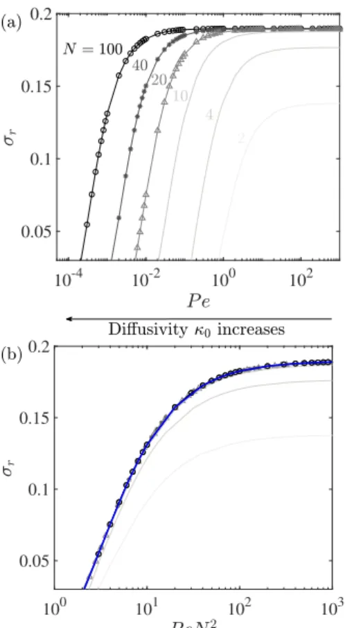
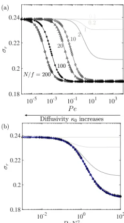
width of the outer annulus of opposite vorticity, the larger the number of unstable azimuthal modes. This might be under- stood by drawing an analogy with plane shear layers.

In the infrared range, the main physical phe- nomena affecting the signal emitted by the scene are shade effect, wind disturbance linked to landscape relief, and

NOTE : ces soirées de formation sont réservées au membres actifs et aux membres résidents

Die infrarote Leuchtdiode LED] wird über die Strahlteiler (halbdurchläßige Spiegel) ST1, ST2, die Linse L2, den Strahlteiler ST3 und die Optik des Auges auf die Netzhaut in

In both dimensions the effect of an increasing pressure-compressibility product is to decrease the sound speeds and Debye temperatures, with a given value of the

Temperature Dependence of the Temperature-driven Oli- gomer-Monomer Relaxation Kinetics— To study the tem- perature dependence of the thermally induced oligomer dis- sociation

Comparison between expected phase and estimated phase when the Iris-AO is flat except for the central segment on which a 225 nm piston is applied, in presence of the Lyot

Pour toutes ces raisons, par souci d’équité, le Conseil tient à souligner la nécessité de considérer l’ensemble des circonstances actuelles : celles dans