Velocity model building by full waveform inversion of early arrivals & reflections and case study with gas cloud effect

HAL Id: tel-01556584

https://tel.archives-ouvertes.fr/tel-01556584

HAL is a multi-disciplinary open access archive for the deposit and dissemination of sci-entific research documents, whether they are pub-lished or not. The documents may come from teaching and research institutions in France or

L’archive ouverte pluridisciplinaire HAL, est destinée au dépôt et à la diffusion de documents scientifiques de niveau recherche, publiés ou non, émanant des établissements d’enseignement et de recherche français ou étrangers, des laboratoires

early arrivals & reflections and case study with gas cloud

effect

Wei Zhou

To cite this version:

Wei Zhou. Velocity model building by full waveform inversion of early arrivals & reflections and case study with gas cloud effect. Earth Sciences. Université Grenoble Alpes, 2016. English. �NNT : 2016GREAU024�. �tel-01556584�

THÈSE

Pour obtenir le grade de

DOCTEUR DE L’UNIVERSITÉ DE GRENOBLE

Présentée par

Wei ZHOU

Thèse dirigée par Romain Brossier, Stéphane Operto et Jean Virieux préparée au sein de l’Institut des Sciences de la Terre

et de l’École Doctorale Terre Univers Environnement

Velocity Model Building by

Full Waveform Inversion of

Early Arrivals & Reflections and

Case Study with Gas Cloud Effect

30 Septembre 2016 , devant le jury composé de :

Hervé Chauris (Président du jury)

Professeur à MinesParisTech, Fontainebleau, Rapporteur

René-Édouard Plessix

Chercheur Principal (HDR) à Shell, Pays-bas, Rapporteur

Gilles Lambaré

Directeur de Recherche à CGG, Massy, Examinateur

François Audebert

Coordinateur R&D à Total, Pau, Examinateur

Romain Brossier

Maître de conférences à l’Université Grenoble-Alpes, Directeur de thèse

Stéphane Operto

Directeur de Recherche au CNRS, GéoAzur, Université de Nice-Sophia Antipolis, Valbonne, Directeur de thèse

Jean Virieux

Acknowledgement

“Boom, boom, booom!” The artificial firework has lighted the night of Grenoble. Like every year the ceremony of the French national day ends with its climax, and this is the third time that I enjoy this kind of fire show. It is amazing that I have been living in this foreign city, made new friends, tasted exotic food, enjoyed a different culture and more importantly accomplished a PhD project with the help of my wonderful supervisors.

I am very grateful to Pr. Jean Virieux for giving me opportunities to do an internship and the following PhD in the frame of SEISCOPE. Jean is an erudite scholar and he always likes to share his knowledge with others. I enjoy every discussion with him and have benefited a lot from that. (I still remember our talk related to Fresnel and Fraunhofer optics.) Giving much advice after my presentations and writing numerous comments and annotations in my manuscripts, I can feel his serious attitude and also kind heart to me. I always appreciate his every encouragement.

Also, I appreciate very much the instructions of St´ephane Operto, who is rigorous in my results and writings, but also very patient to explain the ideas for me. Because we use emails to contact, sometimes it is not easy for him to follow the discussions. Nevertheless, he keeps taking care of my advances and asking if I have any difficulties. I feel very sorry to him that I did not send him emails so frequently as he asked. Many thanks to him for providing me the real data set, and more importantly his FWI result such that I can make the assessment of my result.

Special thankfulness is devoted to Romain Brossier, for his useful instructions and inspirations each time I am obstructed by misunderstandings and difficulties. As a supervisor, he is more like a good friend of mine. I can recall the moment that we looked for beers on the streets of Denver, and the relaxing time but became insensitive for me in Amsterdam. I am very grateful to him for helping me contact Total, manage plane tickets, hold the committee of this thesis and improve the manuscript when he is also occupied by running the consortium.

I want to express my sincere gratitude to the reviewers: Herv´e Chauris (MinesParis-Tech) and Ren´e-´Edouard Plessix (Shell), as well as other members of the committee: Gilles Lambar´e (CGG) and Fran¸cois Audebert (Total). Thank you for your time. I am looking forward to meeting and discussing with you during my defense!

Many thanks to my dear colleagues and friends that have encouraged and supported me in the past years. I enjoy very much the discussions with Ludovic M´etivier, and also his enthusiastic drum shows. I also appreciate his questions and insightful comments on

me the special person the second day he knew me. I also want to express my gratitude to Pengliang Yang for the fruitful discussions, which greatly help me accomplish the real-data application. I enjoy very much his handy viscous inversion code as well as his beautiful calligraphy. I also want to acknowledge Guanghui Hu for contacting the accommodation in Grenoble before I arrived. I want to acknowledge my dear colleagues and friends Amir Asnaashari, Boussad Beldjenna, St´ephen Beller, Fran¸cois Bretaudeau, C´ecile Brouyant, Clara Castellanos, Laure Combe, John Diaz, Michel Dietrich, Longfei Gao, St´ephane Garambois, Andrzej G´orszczyk (Polish academy of sciences), Okba Hami-tou, Fran¸cois Lavou´e, Philippe Le Bouteiller, Isabella Masoni, Himanshu Midha, Alain Miniussi, Vadim Monteiller, Benjamin Pajot, Hugo Pinard, Alessandra Ribodetti, Josu´e Tago, Borhan Tavakoli, Phuong-Thu Trinh, Rapha¨el Valensi (OPERA), Paul Wellington and Huan Zhang. It has been a wonderful period to work with you. I appreciate the assistance and technical support from Magali Gardes, St´ephanie Mandjee and Sandrine Nadau as well as Hafid Bouchafa, Kamil Adoum and Jacque Pellet. I also appreciate the information provided by Christian Bigot and Guy Delrieu. I acknowledge the finan-cial support from the SEISCOPE consortium as well as the HPC resources provided by CIMENT and CINES/IDRIS.

In addition, I want to thank my lovely friends who have supported me in the four-year life. Some of them are also in a PhD project or have finished it, giving me broader views and different ideas. Some of them are fans of football games like me, spending wonderful time together. I give my sincere acknowledgement to Jing He, Gang Li, Zhaohua Li, Bin Ma, Qiuliang Yu, Chao Yuan, Qiujuan Wang, Xinjiletu Zhao, Huaxiang Zhu, Yongliang Chang, Xinteng Gao, Tian Sun and others. I also want to thank Oph´elie Passemard, Delphine Toihir, Nicole Coste and all the Ducros’ for their understanding and kind assistance these days.

Living at another end of the continent makes me homesick, especially when all family members gather together to celebrate a traditional Chinese festival. I am deeply grateful to my parents and other elder relatives for bringing me up, telling me the truth of life, helping me follow dreams and supporting me to do PhD in a foreign country. These years I cannot stay long with them and their bright faces in my mind have become wrinkly and old. I hope in the near future, when I have a permanent location, I can see them more frequently and do whatever I can do. The gratitude is also for my master degree supervisor, Pr. Zhenxing Yao (IGGCAS), and former colleagues, Jinghai Zhang (IGGCAS) and others, who brought me into the field of geophysics and taught me how to do research. Thank you for your inspirations!

At last, I want to acknowledge my little girlfriend Lingzhu Xu. It is my greatest fortune and proud to meet you, date you, kiss you and finally marry you. Thank you for your consistent and endless care of me. You will be the most important and attractive research in my whole life!

Wei Zhou July, 2016

The thesis is based on the following work primarily done by W. Zhou1 _{during his PhD}

study from 04.2013 to 10.2016: Technical reports:

ˆ Zhou, W. (2013). Toward large-scale imaging by reflected Waves: An analysis of wavenumber sampling of reflection FWI, Technical Report No 61, SEISCOPE Project;

ˆ Zhou, W. (2014). Combining diving and reflected waves for velocity model build-ing by waveform inversion, Technical Report No 65, SEISCOPE Project;

Proceedings:

ˆ Zhou, W., Brossier, R., Operto, S. et Virieux, J. (2014). Combining diving and reflected Waves for velocity model building by waveform inversion. In Expanded Abstracts, 76th EAGE Annual Meeting (Amsterdam), We E106 15; ˆ Zhou, W., Brossier, R., Operto, S. et Virieux, J. (2014). Acoustic

mul-tiparameter full waveform inversion of diving and reflected waves through a hier-archical scheme. 84th _{SEG Technical Program Expanded Abstracts (Denver), Page}

1249–1253;

ˆ Zhou, W., Brossier, R., Operto, S. et Virieux, J. (2016). Joint full wave-form inversion of early arrivals and reflections: a real OBC case study with gas cloud. 86th _{SEG Technical Program Expanded Abstracts (Dallas);}

Publications:

ˆ Zhou, W., Brossier, R., Operto, S. et Virieux, J. (2015). Full waveform inversion of diving and reflected waves for velocity model building with impedance inversion based on scale separation. Geophysical Journal International, 202:1535– 1554;

ˆ Zhou, W., Brossier, R., Operto, S., Virieux, J. et Yang, P. (2016). Joint full waveform inversion of early arrivals and short-spread reflections: a 2D ocean-bottom-cable study including gas cloud effects. To be submitted.

Abstract

Full waveform inversion (FWI) has attracted worldwide interest for its capacity to es-timate the physical properties of the subsurface in details. It is often formulated as a least-squares data-fitting procedure and routinely solved by linearized optimization methods. However, FWI is well known to suffer from cycle skipping problem making the final estimations strongly depend on the user-defined initial models. Reflection wave-form inversion (RWI) is recently proposed to mitigate such cycle skipping problem by assuming a scale separation between the background velocity and high-wavenumber re-flectivity. It explicitly considers reflected waves such that large-wavelength variations of deep zones can be extracted at the early stage of inversion. Yet, the large-wavelength information of the near surface carried by transmitted waves is neglected.

In this thesis, the sensitivity of FWI and RWI to subsurface wavenumbers is revis-ited in the frame of diffraction tomography and orthogonal decompositions. Based on this analysis, I propose a new method, namely joint full waveform inversion (JFWI), which combines the transmission-oriented FWI and RWI in a unified formulation for a joint sensitivity to low wavenumbers from wide-angle arrivals and short-spread reflec-tions. High-wavenumber components are naturally attenuated during the computation of model updates. To meet the scale separation assumption, I also use a subsurface pa-rameterization based on compressional velocity and acoustic impedance. The temporal complexity of this approach is twice of FWI and the memory requirement is the same.

An integrated workflow is then proposed to build the subsurface velocity and impedance models in an alternate way by JFWI and waveform inversion of the reflection data, re-spectively. In the synthetic example, JFWI is applied to a streamer seismic data set computed in the synthetic Valhall model, the large-wavelength characteristics of which are missing in the initial 1D model. While FWI converges to a local minimum, JFWI succeeds in building a reliable velocity macromodel. Compared with RWI, the involve-ment of diving waves in JFWI improves the reconstruction of shallow velocities, which translates into an improved imaging at greater depths. The smooth velocity model built by JFWI can be subsequently taken as the initial model for conventional FWI to inject high-wavenumber content without obvious cycle skipping problems.

The main promises and limitations of the approach are also reviewed in the real-data application on the 2D OBC profile cross-cutting gas cloud. Several initial mod-els and offset-driven strategies are tested with the aim to manage cycle skipping while building subsurface models with sufficient resolution. JFWI can produce an

accept-angle illumination provided by 3D acquisitions would allow me to start from cruder initial models.

R´

esum´

e

L’inversion des formes d’onde (full waveform inversion, FWI) a suscit´e un int´erˆet dans le monde entier pour sa capacit´e `a estimer de mani`ere pr´ecise et d´etaill´ee les propri´et´es physiques du sous-sol. La FWI est g´en´eralement formul´ee sous la forme d’un probl`eme d’ajustement des donn´ees par moindres carr´es et r´esolus par une approche lin´earis´ee utilisant des m´ethodes d’optimisation locales. Cependant, la FWI est bien connue de souffrir du probl`eme de saut de phase rendant les r´esultats fortement d´ependant de la qualit´e des mod`eles initiaux. L’inversion des formes d’ondes des arriv´ees r´efl´echies (re-flection waveform inversion, RWI) a r´ecemment ´et´e propos´ee pour att´enuer ce probl`eme en supposant une s´eparation d’´echelle entre le mod`ele de vitesse lisse et le mod`ele de r´eflectivit´e `a haut nombre d’onde. La formulation de RWI consid`ere explicitement les ondes r´efl´echies afin d’extraire de ces ondes une information sur les variations lisses de vitesse des zones profondes. Cependant, la m´ethode n´eglige les ondes transmises qui contraignant les informations lisses de vitesse en proche surface.

Dans cette th`ese, une ´etude de la sensibilit´e en nombre d’ondes des m´ethodes de FWI et RWI a d’abord ´et´e revisit´ee dans le cadre de la tomographie en diffraction et des d´ecompositions orthogonales. A partir de cette analyse, je propose une nouvelle m´ethode, `a savoir l’inversion jointe des formes d’ondes transmises et r´efl´echies (joint full waveform inversion, JFWI). La m´ethode propose une formulation unifi´ee pour combiner la FWI des transmissions et la RWI pour les r´eflexions, donnant naturellement une sensi-bilit´e commune aux petits nombres d’onde venant des arriv´ees grand-angle et r´efl´echies. Les composantes `a hauts nombres d’onde sont naturellement att´enu´ees par la formula-tion. Pour satisfaire l’hypoth`ese de s´eparation d’´echelle, j’utilise une param´etrisation du sous-sol bas´ee sur la vitesse des ondes de compression et l’imp´edance acoustique. La complexit´e temporelle de cette approche est le double de la m´ethode de FWI classique et la requˆete m´emoire reste la mˆeme.

Une proc´edure d’inversion est ensuite propos´ee, permettant d’estimer alternativement le mod`ele de la vitesse du sous-sol par JFWI et l’imp´edance inversion de formes d’ondes r´efl´echies. Un exemple synth´etique r´ealiste du mod`ele de Valhall est d’abord utilis´e avec des donn´ees de streamer et `a partir d’un mod`ele initial tr`es lisse. Dans ce cadre, alors que la FWI converge vers un minimum local, la JFWI r´eussit `a reconstruire un mod`ele de vitesse lisse de bonne qualit´e. La prise en compte des ondes tournante par la JFWI montre un fort int´erˆet pour la qualit´e de reconstruction superficielle, compar´ee `

d’onde tout en ´evitant le probl`eme de saut de phase.

Les avantages et limites de l’approche de JFWI sont ensuite ´etudi´es dans une ap-plication sur donn´ees r´eelles, venant d’un profil 2D de donn´ees de fond de mer (OBC) recoupant un nuage de gaz au dessus d’un r´eservoir. Plusieurs mod`eles initiaux et strat´ e-gies d’inversion sont test´es afin de minimiser le probl`eme de saut de phase, tout en con-struisant des mod`eles de sous-sol avec une r´esolution suffisante. Sous r´eserve de mettre en œuvre des strat´egies limitant le probl`eme de saut de phase, la JFWI montre qu’elle peut produire un mod`ele de vitesse acceptable, injectant les bas nombres d’onde dans le mod`ele de vitesse. L’am´elioration de l’´eclairage en angles de diffraction fournie par des acquisitions 3D devrait permettre de pouvoir commencer l’inversion par JFWI `a partir de mod`ele encore moins bien d´efinis.

Contents

Acknowledgement i

Abstract v

R´esum´e vii

1 Introduction 1

1.1 Seismic data and scale separation . . . 2

1.2 Velocity inversion principles . . . 6

1.2.1 Forward problem . . . 6

1.2.2 Inverse problem . . . 7

1.2.3 Summary . . . 15

1.3 Imaging the subsurface velocity field . . . 16

1.3.1 Ray-based traveltime tomography . . . 16

1.3.2 Migration velocity analysis (MVA) . . . 17

1.3.3 Full waveform inversion (FWI) . . . 18

1.3.4 Reflection waveform inversion (RWI) . . . 23

1.3.5 Summary and motivation of this study . . . 25

1.4 Contribution of this work and thesis outline . . . 25

2 From FWI to RWI 29 2.1 Forward modeling . . . 30

2.2 Formulations and the cycle skipping issue . . . 31

2.2.1 FWI as a least-squares linearized optimization . . . 31

2.2.2 Velocity-depth ambiguity – Reflection data-induced cycle skipping 33 2.2.3 RWI based on scale separation and mitigation of cycle skipping . 36 2.3 Sampling analysis . . . 38

2.3.1 FWI: preferentially high wavenumber samplings . . . 38

2.3.2 RWI: preferentially low wavenumber samplings. . . 42

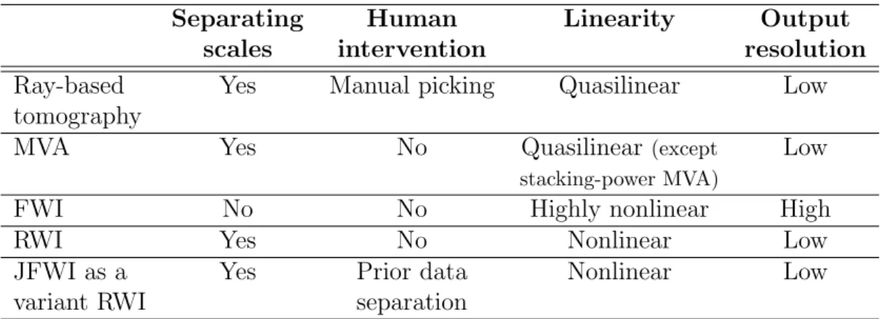
2.3.3 Numerical verification . . . 46

2.4 Discussion . . . 48

2.5 Summary . . . 51

3.1 Introduction . . . 54

3.2 Review of FWI and RWI . . . 58

3.3 Methodology . . . 61

3.3.1 Formulation . . . 61

3.3.2 Mitigation of high-order isochrones by choosing suitable subsurface parameterization . . . 63

3.3.3 Implemention . . . 65

3.4 Integrated workflow of velocity (VP) and impedance (IP) inversion . . . . 67

3.4.1 IP inversion by using short-offset reflection data . . . 67

3.4.2 Cycle workflow of VP–IP imaging . . . 68

3.5 Synthetic example: Valhall case study . . . 69

3.5.1 Experimental setup . . . 69

3.5.2 Results and discussions . . . 71

3.5.2.1 Results and comparisons . . . 71

3.5.2.2 Quality control by common image gathers . . . 73

3.5.2.3 Fitting amplitudes . . . 74

3.5.2.4 Broadband imaging of VP . . . 78

3.5.3 JFWI in presence of multiples . . . 80

3.6 Conclusions and perspectives. . . 84

4 Real Data Application 87 4.1 Introduction . . . 88

4.2 Methodology . . . 90

4.3 Application . . . 92

4.3.1 Preliminary results related to attenuation . . . 96

4.3.2 Inversion setup . . . 99

4.3.3 Results. . . 101

4.3.3.1 Classical FWI . . . 101

4.3.3.2 Joint FWI . . . 105

4.3.3.3 Joint FWI followed by FWI . . . 106

4.3.3.4 Quality control of velocity models . . . 111

4.4 Discussion . . . 113

4.5 Conclusions and perspectives. . . 117

5 Conclusions and Perspectives 119

Bibliography 122

Postscript 145

A Derivation of Gradients through Lagrangian Formulation 149

Chapter 1

Introduction

If I have seen further, it is by standing on the shoulders of giants.

— Isaac Newton, 1676

The mystery of the Earth’s interior has been revealed by earthquake seismology to a much extent. Since the early 1900s, scientists have continuously found that our home planet is rather stratified, with a number of materials under varying pressure and temperature conditions. After a century of development, our knowledge about the underground has been largely enriched, from the physical processes to the chemical compositions, despite an increasing number of questions to be answered.

Since the late 1960s, seismology has also served to prospect the natural resources in the subsurface: a production-oriented branch of seismology that is often termed explo-ration seismology or simply seismics. Modern oil and gas industry has been and will be heavily relied on seismic methods in the foreseeable future. Researches, innovations, applications have brought a golden age of the seismic technology. Though the ideas are similar, the scales of interest are different. While continents, tectonic plates (hundreds of kilometers) or the whole Earth (thousands of kilometers) is the focus of seismologists, local regions on the crust (0.1 to 10 kilometers) are prospected for industrial application. Other differences can be found in Table1.1, with a third type of seismology that will not be discussed in this thesis.

This thesis contributes to the community of exploration seismology, in particular, to its sub-field related to velocity inversion in the acoustic approximation. In this prelim-inary chapter, I shall first introduce some basic principles in seismic imaging followed by the discussion on a group of methods, which are viewed as the starting point of the methodology that I shall describe in Chapter 3.

Table 1.1: Three branches of seismology adopted in different circumstances (adapted from Yilmaz, 2005). Engineering seismology is oriented to the smallest scale with ex-pected higher resolution by considering very high frequencies.

Scale Maximum depth Source type Max. frequency Earthquake continental 100 – 1000 km Passive 10 Hz

seismology global

Exploration local regions 10 km Active 100 Hz

seismology

Engineering local regions 1 km Active or 1000 Hz

seismology passive

1.1

Seismic data and scale separation: a synthetic

example of marine case

Let us start from a synthetic model representative of the Valhall oilfield in the North Sea (Figure 1.1a). The seismic waves are recorded at the surface, a typical acquisition system among others in exploration geophysics. In this 2D setting, the x-axis measures the lateral position of the surface and the z-axis measures the depth from the surface. The yellow star represents one seismic shot, emitting transient mechanic energy into the subsurface. The energy of the excitation spreads out in the space with the form of propagating waves, carrying information of the physical properties of the medium, and captured by a set of receivers deployed at the surface. Figure 1.1b gathers from these grouped receivers the recorded phases (or seismic traces, events) as a function of elapsed time t and horizontal axis x. Relatively, each trace can also be associated with the horizontal distance between the source and receiver of that trace, i.e. the offset h. Note that x and h can be deduced from each other by knowing the source position. Due to the transient excitation, the phases have limited time duration. Due to the wave propagation, we can observe lateral continuity of these phases with certain slopes. Among them, several phases have great importance. The colored arrows identify these phases as well as their associated raypaths connecting the source and receiver for the following interpretation (Figure 1.1b):

1. Transmitted waves from shallow zones:

ˆ Direct wave (green arrows). As the superficial part of the model is homoge-neous (water column), the direct wave follows a straight path;

ˆ Diving wave (green dashed arrows). According to Fermat’s principle, this type of wave follows a curved path that penetrates higher velocity zones at depth so as to arrive at the receiver with shorter time than the direct wave. They are also known as turning wave;

1.1 Seismic data and scale separation a) b) 0 1 2 3 4 5 6 7 8 9 t (s) 0 2 4 6x (km)8 10 12 14 Seismogram x (km) 0 2 4 z (km) 0 2 4 6 8 10 12 14 1.5 2.0 2.5 3.0 (km/s) 0 2 4 z (km) 0 2 4 6 8 10 12 14 1.5 2.0 2.5 3.0 (km/s) 0 2 4 z (km) 0 2 4 6 8 10 12 14 1.5 2.0 2.5 3.0 (km/s)

Figure 1.1: An example of seismic data acquired at the surface. (a) Velocity model. (b) Seismogram recorded by an array of receivers. The yellow start denotes the position of the seismic shot. The wavefield is computed under the acoustic approximation to illustrate only the P waves. The colored arrows identify several phases in (b) and the associated raypaths in (a) that are interpreted in the text.

ˆ Reflected wave. When the wave meets an interface, part of its energy is reflected backwards to the surface, leaving a hyperbolic-like shape (normal moveout) in the seismogram. The blue, red and magenta arrows indicate the reflections occurred on interfaces at 1.5 km, 3 km and 5 km depth, respectively. At far distances, these reflected waves indicated by blue and red arrows tend to be tangent with the diving waves due to the inhomogeneity of overlaying medium. Therefore, we can further classify the reflected waves as precritical (or short-spread) reflection and postcritical (or supercritical) reflection based on their different moveouts;

3. Transmitted waves from deep zones:

ˆ Refracted waves. When the wave meets an interface, part of its energy is for-ward transmitted to deeper layers. As long as the velocity beneath is higher, the wavefront propagating in parallel with the interface serves as secondary sources and generate plane waves propagating to the surface, leaving a nearly straight shape (linear moveout) in the seismogram. This is the case for the 3

phases indicated by the dashed red arrows, associated with the interface at 2.5 – 3 km depths, and the phases indicated by the dashed magenta arrows, associated with the interface at 5 km depth, respectively. At very long dis-tances, these refracted waves can arrive at the surface earlier than the diving waves.

4. Higher-order scattered waves:

ˆ Multiscattered waves (yellow arrows). When in contact with the sharp edges of the embedded blue layers, the reflected wave (red arrows) serves as sec-ondary sources and generates spherical waves that propagate to the surface, leaving a hyperbolic-like shape in the seismogram. As the incident reflected wave is of first-order scattering, these spherical waves are of higher orders. ˆ Multiples (cyan arrows). They are high-order reflected waves that are bounced

back and forth for multiple times between the surface and interfaces (surface-related multiples), or just between different interfaces (internal multiples). In Figure 1.1b, the absorbing surface condition is used to avoid surface-related multiples. Because of the intrinsic energy partition between reflection and transmission, the internal multiples have very weak amplitudes, therefore, they are usually neglected in reflection seismic imaging.

Generally, we are interested in two types of information included in the seismic data: 1. Kinematic information: the traveltime for one phase to propagate from one source

to one receiver, which is a functional of the wavepath and velocity field;

2. Dynamic information: the amplitude of one phase which depends on the source wavelet, the geometrical spreading factor, the dissipation of the medium, and the reflection/transmission coefficients of the interfaces.

In seismic methods, the kinematic and dynamic information is incorporated in different degrees. For example, ray-based tomography methods only use the kinematic property to build a smooth velocity model. Kirchhoff migration relies more on the kinematic than the dynamic to focus the reflector images without properly resolving the reflec-tion/transmission coefficients. Full waveform inversion, on the contrary, simultaneously considers both information for broadband subsurface imaging.

Conventional surface acquisition geometries, such as the streamers in the marine case, often provide insufficient offset and/or azimuth coverage giving small-aperture data. Consequently, the subsurface models we can build lack intermediate wavenumbers in the Fourier domain and provide two parts of the subsurface spectrum. An illustration on the synthetic Valhall model is given in Figure 1.2. This leads to the concept of scale separation that distinguishes between large-scale (low wavenumbers) and small-scale (high wavenumbers) models (Claerbout,1985;Jannane et al.,1989;Wang et Pratt,

1.1 Seismic data and scale separation 0 1 2 3 4 5 6 Wavenumbers (1/m) 8 10 12 14 Log of Amplitude 0 1 2 3 4 5 6 8 10 12 14 Resolution gap Velocity estimation Reflectivity imaging

Figure 1.2: Sketch of the scale-separation assumption (inspired by the famous picture ofClaerbout (1985), figure 1.4-3). As the variations of the subsurface (top) are sampled by seismic waves, we are able to resolve its low-wavenumber part by velocity estimation methods and high-wavenumber part by reflectivity imaging methods, respectively, and this property is termed scale separation in the literature. However, these two parts often do not overlap, leaving the intermediate wavenumbers unsolved. Fourier analysis (bottom) confirms this point, that the true spectrum (black curve) is matched by the reconstructed spectrum (red curve) in the low-wavenumber part (blue area) and the high-wavenumber part (red area) with a resolution gap in the middle.

seismic model with the resolution gap can reproduce the recorded data. The high-wavenumber part is termed reflectivity while the low-high-wavenumber part is termed (macro) velocity model. Depending on the objective, seismic imaging methods can be divided into two categories following Wapenaar (1996):

1. Reflectivity imaging (or seismic imaging, migration), which aims to image the high-wavenumber part, or more specifically aims to resolve the reflection/transmission coefficients of the interfaces inferred from the dynamic property of the data; 2. Velocity estimation (or velocity analysis, velocity model building), which aims to

reconstruct the low-wavenumber part inferred from the kinematic property. Here, the term “velocity” specifically refers to the smooth velocity background.

Considering this natural separation due to insufficient acquisition coverage, in the conven-tional seismic processing workflow, the kinematic information is extracted as the initial step to build the large-scale velocity field, followed by seismic imaging of the small-scale reflectivity profile involving the dynamic information. Nevertheless, we should note that such a separation is less true nowadays, because efforts have been taken to recover in-termediate wavenumbers by designing wide-azimuth long-offset acquisition geometries, using high-quality broadband data, and applying high-resolution imaging methods such as full waveform inversion (as reported by Lambar´e et al.,2014).

1.2

Velocity inversion principles

Velocity estimation can be formulated as an inverse problem that “looks for a question which can be responded by the proposed answer”. In particular, the recorded seismic data are the proposed “answer” and the subsurface model is the “question” we want to find. However, before solving this inverse problem, we need to know how to solve the forward problem: given a model, how to compute the synthetic seismic data (“how to answer a given question”). These two problems make up velocity inversion that is often formulated in the frame of optimization theory. In this section, I shall discuss some general principles in solving the forward and inverse problems using waveforms. The mathmatical formulation is deferred until Chapter 2.

1.2.1

Forward problem

Because of their similar kinematic behavior, seismic waves can be treated as optic rays based on high-frequency approximation (Cerven´ˇ y,2001;Chapman,2004;Virieux et Lam-bar´e, 2007). The traveltime of one phase is then computed by the integration of the inverse of local velocities (slowness) along the raypath that connects the source-receiver couple, which is also known as ray-tracing (Zelt et Smith, 1992; Bishop et al., 1985). However, according to Fermat’s principle, low-velocity zones tend to be under sampled by raypaths leading to poor resolution in complex media (Virieux et Farra, 1991). An alternative to tracing rays consists in solving the eikonal equation, a nonlinear partial differential equation that relates the derivatives of traveltime to local velocities (Le Meur et al.,1997). It can be numerically solved either by the fast marching method (Popovici et Sethian, 1998; Leli`evre et al., 2011) or by the fast sweeping method (Vidale, 1990;

Zhao, 2004; Bretaudeau et al., 2014).

Alternatively, one can consider the wave equation to honor the real physics of seis-mic waves. The wave equation is a linear partial differential equation and can be dis-cretized by various schemes (Kelly et al., 1976; Marfurt, 1984; Virieux, 1984; Dablain,

1986; Levander, 1988; Brossier et al., 2008). The finite-difference method (Virieux,

1984; Levander, 1988) is popular for its simplicity and scalability, but generates arti-ficial boundary reflections that are often mitigated by considering absorbing boundary conditions (e.g. perfectly-matching layers, smart layers, B´erenger, 1994; M´etivier et al.,

1.2 Velocity inversion principles

2014b). On the other hand, the finite-element method (Marfurt,1984;Seriani et Priolo,

1994;Min et al.,2003;Dumbser et K¨aser,2006;K¨aser et Dumbser, 2008), which is often more computationally intensive, naturally introduce boundary conditions giving more accurate solutions. By using tetrahedral meshes (Frey et George, 2008) the method can almost perfectly fit complex topographies, and the mesh width can be locally adapted to medium properties.

On the other hand, image-domain velocity inversion, as well be described later, con-siders the reflectivity images inferred from synthetic data as the solution of its forward problem. In other words, the forward problem for image-domain inversion consists of forward modeling (computes synthetic data) followed by migration (computes reflectiv-ity images). For this reason, the computational cost of image-domain inversion is often larger than its data-domain counterpart. For overviews of migration techniques I refer to Sava et Hill (2009) and Etgen et al. (2009). Likewise, migration can be also based on the ray approximation (Kirchhoff migration,Schneider,1978). The computation load is less heavy than wave equation-based migration; however, the latter one is currently more discussed in the literature for complex-structure imaging. A number of approaches have been proposed. Using the approximate one-way wave equation, the wavefield at one depth can be extrapolated to another depth, and images can be built by the coincident time imaging condition (Claerbout, 1985; Wu,1994; Ristow et Ruhl,1994; Le Rousseau et de Hoop,2001). Alternatively, the wavefield can be computed through time marching methods using the true two-way wave equation (reverse time migration (RTM), Baysal et al.,1983;McMechan,1989). Besides, true amplitude or quantitative migration aims to resolve the reflection/transmission coefficients of interfaces, and the second-order infor-mation can be considered (Lameloise et al.,2015). Least-squares migration is formulated as a linear inverse problem to explicitly solve for the reflectivity (Nemeth et al., 1999). In Chapter3, I shall also propose an RTM-like least-squares waveform inversion to image reflectivity in the impedance parameter.

1.2.2

Inverse problem

Without talking about other methodologies, I mention the following two ways to assess the quality of the velocity model:

1. Data domain, which measures the data fitness to assess the velocity model. If the observed data are well matched by the synthetic data computed in the proposed velocity model (and other parameters such as density), then we regard the proposed model as a reliable representation of the subsurface (i.e. true model);

2. Image domain, which measures the “coherency” of reflectivity images respectively resolved from each source-receiver couple. If the positions of these images are independent of the source-receiver offset (or other acquisition parameters that are not a model attribute), then we regard the proposed velocity model as the true model. Other “coherency” criteria have also been proposed.

Therefore, any data mismatch (in the data domain) or image incoherency (in the image domain) are attributed to velocity inaccuracies, and can be used to update the velocity model. Usually, the relationship between the velocity model and the data match or image coherency is nonlinear, but we still apply local optimization schemes to solve the inversion problem due to its large size. In the following, I shall show how full waveform inversion (FWI) and reflection waveform inversion (RWI), representatives of data-domain methods, transform their respective data misfit into model update through the gradient computation flow. After this, image-domain methods will also be described using an example of common image gather (CIG).

Data domain velocity inversion: FWI case

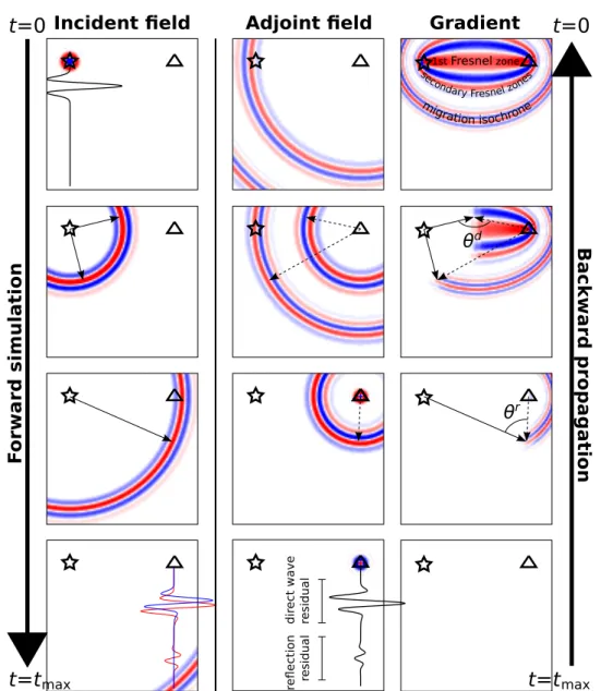
Figure 1.3 illustrates how we build the FWI gradient based on wavefield simulation. Suppose that we have estimated the source wavelet of the observed waves (black wiggle in top left panel). We can simulate the propagation of the incident wavefield (blue-white-red color scale) in the proposed model (left panels). Suppose this model is homogeneous and isotropic, then the wavefront has a circular shape (solid arrows in left panels) with the source position (stars) as its center. We sample the wavefield at the receiver position (triangle) and compare it with the observed wavelet often sample by sample (blue vs red wiggles).

This forward modeling process is followed by a back propagation process which com-putes the adjoint field (middle panels) and the gradient (right panels) to convert the data misfit into model update. For simplicity I take the classical L2 norm-formulated FWI which implies the difference between modeled and observed data (i.e. the data residu-als) to be the adjoint source of the adjoint field (black wiggle in bottom middle panel). Based on the formulation which will be present in Section2.2, the adjoint field should be computed in the reverse time order as indicated by the right-most upward thick arrow. Suppose we have two separated signals in the residuals which are associated to direct and reflected waves, respectively, then we generate two wavefronts in the adjoint field. The inner one comes from the direct wave while the outer one from the reflected wave.

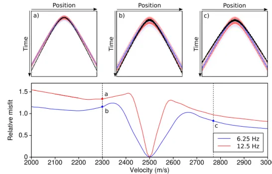
The gradient is formed by pixel-to-pixel zero-lag cross-correlations between the cident and adjoint fields. The direct wave-associated wavefront in the adjoint field in-terferes with the incident wavefront where their wavenumber vectors (dashed and solid arrows in right panels, respectively) make the open angle (θd_{) nearby 180}◦_{. According to}

the diffraction tomography principle, the magnitude of the imaging wavenumber vector formed by such interference is inversely proportional to the cosine of θ. Consequently, the direct wavefront and its adjoint counterpart generate several isophase elliptic zones in the gradient map with large-wavelength variations along the direct wavepath between the source and receiver, the inner-most of which is known as the first Fresnel zone and others are known as secondary Fresnel zones (red and blue elliptic zones).

On the other hand, the reflected wave-associated wavefront in the adjoint field inter-feres with the incident wavefront where their wavenumber vectors make the open angle (θr_{) nearby 0}◦_{. Consequently, they contribute to small-wavelength components inside}

1.2 Velocity inversion principles the reflection-associated secondary Fresnel zone, in an elliptic shape with the source and receiver as the focal points, which is also known as the migration isochrone (Tarantola,

1984; Lailly, 1984).

The gradient is stacked over all source-receiver couples (e.g. Figure 1.5a for the Val-hall model), and is scaled to update the velocity model. The gradient consists of the large-wavelength component, coming from the transmitted waves (direct, diving and re-fracted waves), and the small-wavelength component, coming from the reflected waves. As a result, in FWI, we do not assume scale separation and we are looking for a broad-band image of the subsurface. However, because of the surface acquisition geometry, we can only record a part of the transmitted waves that travels in a limited depth of the subsurface, and the large-wavelength component of the gradient are concentrated in the shallow zone of the subsurface. The small-wavelength component, on the contrary, is distributed at all depths (they are overlaid by large wavelengths in shallow zone but we do have the sensitivity there).

To mitigate the lack of large-wavelength component in depth, one often looks for larger offsets to record diving waves passing through greater depths. However, this is not efficient: an empirical relation states that the penetration depth of diving waves is only one third to one sixth of the largest offset; we may need an acquisition length more than twenty kilometers in order to record the diving waves that sample the targets at the reservoir level. Using lower frequencies in another solution because it brings lower wavenumber content from the migration isochrone. However, since the source wavelet is band-limited we would be obstructed by the noise in the low-frequency end.

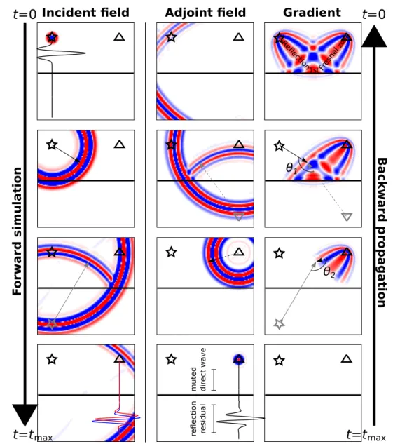
Data domain velocity inversion: RWI case

Large-wavelength updates can be extracted from reflected waves which naturally ex-tends to great depths (Figure 1.4). This is achieved in RWI by generating reflection wavefields during both forward and backward modeling processes using prior reflectors. To clarify which wavefront is mentioned, I shall adopt the words “downgoing” and “up-going” although the wavefront does not propagate only in the vertical direction.

During forward modeling, the downgoing incident field interacts with the reflector (black line in the model) and generates the upgoing reflection field. Due to the energy partition on the reflector, this upgoing field is weaker than the downgoing field. The upgoing field has a semicircle wavefront that is symmetric to the wavefront of the down-going field. Considering such symmetry, we can denote the wavenumber vector of the upgoing wavefront (gray arrow) by assuming a virtual source (gray star) at the mirror position of the real source (black star) with regard to the black line.

The whole incident wavefield (both downgoing and upgoing) is sampled at the re-ceiver position (triangle). However, standard RWI only considers the contribution from reflected waves; therefore, the direct wave residual is muted in the adjoint source (black vs red wiggles in bottom middle panel). Similar to the incident field, the adjoint field has also the downgoing and upgoing partition due to the presence of reflector, and the wavenumber vector of the upgoing wavefront (dashed gray arrow) can be denoted by as-9

Incident field Adjoint field Gradient Backwa rd p ropa gat ion F orwa rd si mul atio n θr 1st Fresnel zone t=0 t=0 t=tmax t=tmax

migra_{tion isochro}ne

sec

ondary Fresnel zones

dir ect wa ve residual re fl ect ion residual θd

Figure 1.3: Time-domain FWI gradient computation animation. Incident field (left panels) by forward simulation (top to bottom panels), adjoint field (middle panels) and gradient (right panels) by backward propagation (bottom to top panels), plotted in the blue-white-red color scale. Stars and triangles denote the source and receiver positions, respectively. In the homogeneous isotropic model, the wavefronts have a circular shape centered at the source or receiver position. Their wavenumber vectors are denoted by arrows. Two angles are made: 1) θd_{between vectors of the incident wavefront and adjoint}

wavefront coming from direct wave; 2) θr between vectors of the incident wavefront and adjoint wavefront coming from reflected wave. Because of their different angle ranges, large-wavelength Fresnel zones are formed along the direct wavepath between source and receiver, whereas small-wavelength migration isochrone (reflection-associated Fresnel zone) is formed in an elliptic shape with the source and receiver as the focal points. Online animation: https://drive.google.com/open?id=0Bx0JCm2KZyuebXI5M2lYTW8tLTg

1.2 Velocity inversion principles

Incident field Adjoint field Gradient

Backw a rd propagat ion F orward simulatio n θ2 t=0 t=0 t=tmax t=tmax Fresne l zon e Re_flecti on 1st θ1 re fl ection resid ual muted dir ect w a ve

Figure 1.4: Time-domain RWI gradient computation animation. Incident field (left panels), adjoint field (middle panels) and gradient (right panels) same as in Figure 1.3. Black stars and triangles denote the source and receiver positions, and gray stars and triangles denote the mirrored positions, respectively. Direct wave is muted at receiver. Both incident and adjoint fields are scattered due to the existence of reflector. The wavenumber vectors associated to downgoing wavefronts are denoted by black arrows, and the ones associated to upgoing wavefronts are denoted by gray arrows, respectively. Two angles are made: 1) θ1between vectors of downgoing incident wavefront and upgoing

adjoint wavefront; 2) θ2 between vectors of upgoing incident wavefront and downgoing

adjoint wavefront. Because of their large angles, large-wavelength Fresnel zones are formed along reflection wavepath between surface and reflector. In this animation, I have filtered out the migration isochrone that was generated by the two downgoing wavefronts. Online animation: https://drive.google.com/open?id=0Bx0JCm2KZyueM25GMF96STJ3QWs

Shallow zones Deep zones

a) b)

Figure 1.5: FWI (a) and RWI (b) gradients stacked over surface acquisition in the Val-hall case. Smooth initial models are used. Migration is implemented before RWI to image reflectivity. For FWI gradient, large-wavelength components coming from trans-mitted waves are concentrated in shallow zones, whereas small wavelengths coming from reflected waves are distributed in the whole space. In contrast, RWI aims to build a smooth velocity model by using reflected waves, which can remedy the large-wavelength shortage of FWI gradient in deep zones.

suming a virtual receiver (gray triangle) at the mirror position of the real receiver (black triangle) with regard to the black line.

In the right panels, the upgoing wavefront in the incident field interferes with the downgoing wavefront in the adjoint field making an open angle (θ2) nearby 180◦.

Simi-larly, the downgoing wavefront in the incident field interferes with the upgoing wavefront in the adjoint field making another open angle (θ1) also nearby 180◦ (notations to be

consistent with Section 2.3). Consequently, they contribute to large-wavelength compo-nents inside the reflection-associated Fresnel zones along the two-way wavepath between the surface and reflector followed by the reflected wave. Therefore, we can recover large-wavelength variations above the deepest reflector.

On the other hand, the interference of the two downgoing wavefronts in the incident and adjoint fields should have generated the small-wavelength migration isochrone as shown in the FWI gradient. However, we intentionally remove this component because the formalism of the RWI gradient does not include this component (see Chapter 2). We can do this because we can explicitly reproduce the migration isochrone (to the first order at least) through the FWI gradient computation process using only the reflected wave residual and the reflector-free model. In this way, the actual computation of the RWI gradient amounts to compute four wavefields and double time complexity of the FWI gradient. As a result, the RWI gradient is dominated by its large-wavelength components. The stacked gradient for the Valhall model is shown in Figure 1.5b.

Both FWI and RWI rely on data mismatch to update the subsurface model. How-ever, they differ in two main aspects: 1) Unlike FWI, RWI adopts the scale-separation assumption in which the prior reflector is fixed during inversion iterations whereas the smooth velocity is the aim to be updated; 2) RWI relies on reflected waves to image the long wavelengths in deep zones whereas FWI relies on diving waves to do this job but only limited to shallow zones. In Chapter 2, I shall provide a detailed analysis and complete explanation of the FWI and RWI gradients.

1.2 Velocity inversion principles Time (ms) Position x on surface (m) Offset 2h (m) 0 500 1000 1500 2000 2500 3000 4000 5000 6000 1000 2000 7000 8000 9000

a)

A

B C

b)

D

E F

Figure 1.6: Velocity inversion in image domain (adapted fromChauris,2000). 3D presen-tation of the time-domain seismic data computed in 2D Marmousi model (a), converted to surface-offset depth-domain common image gathers (b) by prestack depth migration using the true velocity model. A,D: prestack zero-offset common offset gather; B,E: common midpoint gather; C,F: prestack common offset gather collected at largest offset. Accurate velocity model results in flat images across offsets (E). Conversely, residual moveout of migrated images can be used to update the velocity model.

Image domain velocity inversion

Image-domain methods rely on the fact that the data space is always larger than the model space. Take the 2D geometry as an example, we want to build a 2D model (dimensions of z and x) from a 3D data set (dimensions of t and two spatial locations regarding the shot and receiver). Although in the case of multiparameter inversion more 2D models are simultaneously built, we still enjoy an over-determination property of the inverse problem.2 Therefore, we can use such data redundancy to quality control the

2_{Note that this is not to say solving this inverse problem is easy. On the one hand, the relation}

be-tween the wavefield and the propagation medium is nonlinear therefore linearized optimization methods often converges to a local minimum. On the other hand, deep targets are insufficiently sampled

velocity model and update it.

Among different variants I shall describe the flatness criterion derived from the surface-offset common image gathers. Figure 1.6a shows three profiles of the seismic data computed in the Marmousi model. Profile A shows the prestack common offset gather collected at zero offset. The continuous reflection phases (e.g. black line) indicate a series of reflectors in the subsurface, and the scattered waves with a hyperbolic shape (black arrows) indicate point diffractors located on reflector discontinuities. Profile B shows the common midpoint gather collected at a surface position (fixed x). The normal moveout of the reflected waves, i.e. the behavior of later arrivals at larger offsets, is a typical kinematic information for velocity estimation. In the common offset gather collected at the largest offset (Profile C), the reflection phases are recorded in a rather short time window, hence are hard to be interpreted.

Prestack depth migration converts these time-domain data into depth-domain reflec-tivity images (Figure1.6b, note the different vertical axis). If the accurate velocity model is used, the reflection phases in the common offset gathers are reshaped by migration and should be transferred to the associated reflector positions (comparing A and D in Figure

1.6). For example, the phases (black line) arrive later than 2 s in Profile A are reshaped to be a flat reflector image at 2500 m depth in Profile D. The flanks of the hyperbolic scattered waves (arrows in A) are refocused on the associated reflector discontinuities (arrows in D), indicating the fault structure at shallow depth. Similar to the FWI case, larger offsets provides lower wavenumber components, therefore the reflectivity image in Profile F is less sharp as the image in Profile D. By stacking over offsets, a broadband image (including more high wavenumbers) can be built for geological interpretation.

When the proposed velocity model is inaccurate, we cannot stack over offsets due to the destructive stack between low- and high- wavenumber images. Conversely, we can assess the velocity model by measuring their consistency: if the velocity is accurate, the reflectivity images should be positioned at the same depth across offset (e.g. flat images as shown in Profile E); otherwise any depth inconsistency (i.e. residual moveout) indicates an erroneous velocity background and thus can be used to update the velocity model. Note that only one common midpoint gather collected at a fixed position (e.g. Profile E) is not sufficient to update the velocity model in the whole space. Therefore, sufficient amount of common midpoint gathers that are averagely sampled on the surface should be considered, which inevitably causes a large consumption of the memory space. The common midpoint gather mentioned above is one possibility of what is referred to as common image gathers (CIGs) in image-domain methods. Other CIGs, such as the angle-domain CIG and the subsurface-offset CIG are also proposed to reduce the nonuniqueness of the inverse problem, and to facilitate an automatic consistency mea-surement. A discussion will be devoted to this topic in Section 1.3.2.

Migration is implemented in both RWI and image-domain methods. They both aim to update the smooth velocity based on the scale-separation assumption. However, they

time only by precritical reflected waves) making imaging at this depth very ill-posed. See a real-data example in Chapter4 that is encountered in my PhD study.

1.2 Velocity inversion principles

Table 1.2: Classification of velocity inversion methods based on how the forward and inverse problems are solved, arranged in rows and columns, respectively (adapted from

Jones, 2010). Examples are provided in each entry with full names given in the text.

Data domain Image domain

Ray based FATT, RTT Prestack migration

(purely kinematic) tomography

Waveform based Finite-frequency tomography, MVA (kinematic + dynamic) FWI, RWI, JFWI

differ in two main aspects: 1) Unlike RWI, image-domain methods consider the image inconsistency rather than data misfit to update the velocity model; 2) The migration image for RWI is independent on offset whereas multiple image profiles are built for each offset in image-domain methods. In other words, the dimension of the image for RWI is smaller than that for image-domain methods, therefore requires less memory space and shorter computational time.

1.2.3

Summary

Depending on how the forward and inverse problems are solved, velocity inversion meth-ods can be classified into four categories (Table 1.2). In first arrival traveltime tomog-raphy (FATT) and reflection traveltime tomogtomog-raphy (RTT), seismic waves are approx-imated as high-frequency rays and only traveltime information is used to update the model. They cannot provide high-resolution images especially in complex media, and the dynamic information should also be considered. Possible options include the finite-frequency traveltime tomography that measures the time delays by cross-correlation of waveforms, or standard FWI and RWI directly that directly computes the data misfit. On the other hand, migration is also included in the forward problem of image-domain methods, which can be based either on ray approximation or on wave equation. The latter one is also known as migration velocity analysis (MVA), which is currently a hot topic in the literature. In general, because the associated objective functions are more convex than the waveform-based objective function associated to data-domain methods, MVA is more robust in practice (Symes, 2008). Nevertheless, particular data domain methods are also proposed that promise similar stability as MVA (Cl´ement et al., 2001;

Chauris et Plessix, 2012; Chavent et al., 2014;van Leeuwen, 2010; Gao et al., 2014). The method proposed in this thesis, namely joint full waveform inversion (JFWI), is a waveform-based data-domain method for velocity inversion. It combines FWI and RWI for large-wavelength imaging whereas small-wavelength contribution is suppressed. In the next section, as a preamble of JFWI, I shall discuss on ray-based traveltime tomography, MVA, FWI and RWI in more details. The introduction of JFWI will be given in Chapter3 after a theoretical analysis in Chapter 2.

1.3

Imaging the subsurface velocity field

1.3.1

Ray-based traveltime tomography

Ray-based traveltime tomography aims to update the velocity model by using the trav-eltimes of seismic phases. As already mentioned, the synthetic travtrav-eltimes can be com-puted by either ray-tracing or solving the eikonal equation. On the other hand, the observed traveltimes are often manually picked from the recorded data based on a prior phase identification. Picking the first breaks in the seismic data, first arrival traveltime tomography (FATT) relies on traveltimes of diving and refracted waves (Zelt et Barton,

1998; Toomey et al., 1994). This method is also widely adopted in global seismology because the very-far acquisition systems can provide significant transmitted waves that have passed through deep zones (Bijwaard et Spakman, 2000; Montelli et al., 2004a,b). However, by surface acquisition deep targets are insufficiently sampled by transmitted waves due to the limited offset range. In contrast, reflection traveltime tomography (RTT) relies on the traveltimes of reflected waves that better sample deep targets. Sim-ilar to reflection waveform inversion, reflectivity images should be built explicitly such that the synthetic traveltimes of reflected waves can be computed (Bishop et al., 1985;

Sword,1987;Farra et Madariaga,1988;Whiting,1998). The traveltime residuals are then used to update both the velocity and reflector depths, introducing the dilemma between vertical velocities and depth positions of interfaces. Nevertheless, since the transmitted and reflected waves sample in different depth ranges and contribute to distinguished ve-locity update, combinations of FATT and RTT have been proposed for a better veve-locity modeling building (Zelt et Smith, 1992;Hobro et al.,2003; Huang et Bellefleur, 2012).

However, picking the reflection traveltimes in the observed data is often difficult. For example, early reflection phases with large slopes could interfere with late ones with small slopes at far offsets, therefore makes the late phase picking troublesome. To overcome this issue, stereotomography is promoted to pick locally coherent seismic events characterized by their slope which is done in a semi-automatic way (Billette et Lambar´e,

1998; Billette et al., 2003;Lambar´e et al.,2004; Lambar´e,2008). Moreover, because the slope is a kind of kinematic information that is independent of traveltimes, it provides additional constraints for velocity model building. At the beginning, the method was applied to reflected waves, but extensions to converted waves (Alerini et al., 2007; Nag et al.,2010) and transmitted waves (Gosselet et al.,2005; Prieux et al.,2013c) have also been proposed.

The development of ray-based traveltime tomography is reviewed byWoodward et al.

(2008) and Lambar´e et al. (2014). Among all efforts, the main is the hunting for high resolution. Waveform inversion could be a substitute of traveltime tomography for this purpose. However, as the relation between waveform and velocity is highly nonlinear, waveform inversion is generally less stable in practice. Therefore, combing tomography and waveform inversion is more robust to reach the high resolution. One possibility is to build the large wavelengths of the velocity model by traveltime tomography before imaging fine structures by waveform inversions (e.g.Prieux et al.,2013c;Vigh et al.,2016;

1.3 Imaging the subsurface velocity field

Gorszczyk et al., 2016). Another possibility is to perform tomography and waveform inversion simultaneously (e.g. Zhang et al., 2014; Treister et Haber, 2016). The weights between the two should be tunable by the user to emphasize one method over another.

The principle that local slopes can be used to update the velocity model is not lim-ited to stereotomography; a connection of stereotomography with differential semblance optimization (an MVA method) has been highlighted bySymes (2008);Chauris et Noble

(2001). In parallel with tomography, MVA has served as an alternative approach for velocity model building, which is discussed as follows.

1.3.2

Migration velocity analysis (MVA)

Migration velocity analysis relies on the data redundancy to build the velocity model. Prestack migration is performed to generate a certain common image gather (CIG) such that the quality of velocity model can be assessed. As shown in Figure1.6, surface-offset CIG (SOCIG) is built by gathering migration images from each source-receiver offset. The flatness of images is conventionally quantified by the stacking power condition (or semblance criterion Al-Yahya, 1989; Plessix et al., 2000; Soubaras et Gratacos, 2007), which sums the image across offset. Although it attributes a maximum power to the cor-rect model, the objective function is highly oscillatory due to the constructive interference of unrelated images at different offsets, leading to anomalously high powers for incorrect velocities (Chauris et Noble, 2001). This is a similar case with conventional FWI that the inversion can be easily trapped into local minima of the non-convex L2 norm-based misfit function (See Section 1.3.3). To overcome this issue, Symes et Carazzone (1991) propose to locally measure the derivative of image with respect to the offset in an au-tomated way (differential semblance optimization, DSO), and they are able to show, in the 1D case, the DSO objective function is essentially quadratic, a very good property for local optimization method to find the global minimum (Symes,1999). Extensions to 2D case have been performed byChauris et Noble(2001);Mulder et Ten Kroode(2002);

Shen (2004); Albertin et al.(2006); Shen et Symes (2008). Their successes confirm that this property still holds in realistic applications.

One shortage of SOCIG is that, when the velocity model is inaccurate, the gather may not preserve all the reflection energy after migration, especially when the offset range is limited. One solution is to extend the image space such that unfocused energy can be preserved in the non-physical dimensions of the extended image (the so-called depth-oriented CIG), and then penalize this energy to update the velocity model. Remind that in wave equation-based migration the image is computed by the pixel-to-pixel zero-lag cross-correlation between the source and receiver wavefields (Claerbout, 1985), cross-correlation with temporal lag and/or spatial shift can be used to compute the extended images (Rickett et Sava, 2002;Sava et Biondi,2004; Sava et Fomel,2006; Yang et Sava,

2011; Sava et Vasconcelos, 2011). Using the temporal lag consumes a small amount of memory space, whereas using the spatial shift is more consuming as it can be associated to both vertical and lateral directions. However, because it can bring information from 17

the local slope of events, the lateral shift is often considered in practice leading to the so-called subsurface-offset CIG (SSCIG, Shen et Symes, 2008; Lameloise et al., 2015).

Alternatively, depth-oriented CIG can be formulated in the angle domain (ADCIG), which relates the images to the open angle between the wavenumber vectors of source and receiver wavefronts (Xu et al., 2001; Chauris et al., 2002; Brandsberg-Dahl et al., 1999;

Sava et Fomel, 2003; Biondi et Symes, 2004; Biondi et Tisserant, 2004). Therefore, the velocity update is computed by flattening the images across angles. Although both aim to flatten the images, ADCIG is superior to SOCIG because it can uniquely determine the velocity field (private communication with Pengliang Yang, Stolk et de Hoop,2005). On the other hand, Shen et Symes (2008) prefers SSCIG to ADCIG from a numerical-condition point of view. Constructing ADCIG by ray-based migration is straightforward, as the angle can be easily deduced from the ray parameter that is evaluated during migration (Chauris et al., 2002). However, in order to tackle complex media the wave equation-based migration should be applied, and the resulting SOCIG or SSCIG can be converted to ADCIG via the Radon transform (Sava et Fomel, 2003; Silvestrov et al.,

2016, etc).

While successful applications have been reported, MVA suffers from biases in the objective function and gradient artifacts caused by limited acquisition geometry and complex structures (Fei et Williamson, 2010; Mulder, 2014). Proposed strategies to compensate for this illumination issue include Shen et al.(2011); Yang et al.(2013) etc.

Lameloise et al. (2015) propose quantitative migration by introducing Hessian matrix to mitigate the gradient artifacts. Recent advances of MVA deal with combining trans-mitted waves in MVA for more constraints on near-surface velocities (Lameloise, 2015), using multiples for higher resolution (Berkhout et al.,2015;Cocher et al.,2015), and re-placing the migration process by linearized inversion (inversion velocity analysis) which can also mitigate the gradient artifacts for the velocity update (Liu et al.,2014b;Chauris et al., 2015).

Compared with FWI, the main advantage of MVA is its stable convergence to reliable velocity models. On the other hand, FWI has its reputation of high-resolution results. Nonetheless, researchers have investigated the possibility to combine two methods, hop-ing to reach high resolution in a robust way (e.g. Biondi et Almomin, 2013; Fleury et Perrone, 2012; Allemand et Lambar´e, 2015; Santos et al., 2016). Among them, Biondi et Almomin (2013, 2014) proposed an objective function which combines the L2 norms of data difference (FWI-related) and image unfocusing in SSCIG (MVA-related), such that the true velocity model can be built even if a poor initial model is used.

1.3.3

Full waveform inversion (FWI)

Full waveform inversion was first introduced by A. Tarantola and P. Lailly in 1980s (Tarantola, 1984; Lailly, 1984; Tarantola,1986). They showed that the first iteration of FWI resembles a migration process that produces reflectivity images (Devaney,1984;Wu et Toks¨oz, 1987; Mora, 1989). Due to the restriction to very short offsets at that time,

1.3 Imaging the subsurface velocity field however, they were unable to update the long wavelengths of the model (Gauthier et al.,

1986; Mora, 1988; Jannane et al., 1989; Crase et al., 1990; Pica et al., 1990). In 1990s, the computational load of FWI was reduced by Pratt’s group (Pratt et Worthington,

1990; Pratt et al., 1998; Pratt, 1999) by reformulating FWI in the frequency domain. They pointed out that a reduced set of frequencies is already sufficient to provide a non-biased image of the subsurface (Sirgue et Pratt,2004;Sirgue,2006). For robustness, they applied FWI to cross-well data to favor transmitted waves (Pratt et al., 1996; Pratt et Shipp,1999). With the development of wide-aperture/long-offset acquisition geometries, intermediate wavenumbers of the subsurface can be imaged (Neves et Singh,1996;Shipp et Singh,2002;Sirgue et al.,2007;Wang et al.,2015), making this method unlike others: in principle, it does not assume scale separation between velocity background and high-wavenumber reflectivity. On the other hand, as the dense arrays of receivers provide much larger data volumes than ever, the automatic misfit evaluation in FWI outstrips the cumbersome picking step in traveltime tomography. Thanks to the development of computational infrastructures, we can implement more large-size FWI jobs on clusters, and since 2006 we have witnessed a rapid growth in the number of citations in the literature (Figure1.7), from geophysical prospecting (e.g.Ravaut et al.,2004;Malinowski et Operto, 2008; Plessix, 2009; Sears et al., 2010; Vigh et al., 2010; Prieux et al., 2011;

Plessix et al., 2012; Etienne et al., 2012; Brossier et al., 2013; Gholami et al., 2013a;

Warner et al.,2013;Vigh et al.,2014;Operto et al.,2015;Amestoy et al.,2015;Wellington et al.,2015) to crustal and lithospheric seismology (e.g. Operto et al., 2006;Brenders et Pratt, 2007; Fichtner et al., 2010; Beller et al., 2014). For a nice overview of FWI in exploration geophysics, I refer to Virieux et Operto(2009).

FWI can be implemented either in the time domain or in the frequency domain. In the time domain, the elapsed time is reduced by distributing all shot gathers over the processors of parallel computers. A second level of parallelism can be used for domain decomposition of the computational mesh (Etienne et al.,2010). Nonetheless, such cost can be reduced, at the expense of convergence rate and quality of results, by limiting the number of shots with random selection during FWI iterations (van Leeuwen et Her-rmann, 2012; Warner et al.,2013), or deterministic or stochastic source encoding (Vigh et Starr, 2008; Krebs et al., 2009; Ben Hadj Ali et al., 2011; Bansal et al., 2013; Castel-lanos et al., 2015). Alternatively, FWI can be performed in the frequency domain, in which case the computational cost is proportional to the number of discrete frequencies involved in the inversion. The wave equation transfers to the Helmholtz equation in the frequency domain, which can be solved by direct or iterative solvers (Demmel, 1997). The drawbacks of direct solvers, i.e. the poor scalability and significant in-core memory requirement, can be mitigated by new numerical methods such as block low-rank approx-imation (Amestoy et al.,2015). However, as we move to 3D geometries, the direct solver becomes very resource demanding and we have to apply iterative solvers (Erlangga et Herrmann,2008;Plessix,2009;Li et al.,2014;Hamitou et al.,2015). Hybrid approaches are also promoted to reduce the cost, in which the discrete frequencies are extracted from time-domain seismograms via discrete Fourier transform (Nihei et Li,2007; Sirgue et al.,2008; Brossier et al.,2014). These three strategies have been recently reviewed by

Pajot et al.(2014), who point out the scalability issue remains for the direct and iterative 19

Figure 1.7: Increasing citations of FWI in the literature (from Google Scholar, keyword “full waveform inversion”, 13/05/2016). The numbers include publications, presentations, reports etc., hence give an upper limit of published works in each year. Proposed in 1984, FWI was not widely accepted until 2006, over 200 citations was reached thanks to the upgraded computing hardware. The curve has increased for five times after 9 years. By the end of 2016, a number around 1300 could be anticipated.

solvers. Brossier et al. (2014) compare time-domain FWI and frequency-domain FWI based on time-domain modeling, and show a same temporal complexity for the gradient computation embedded in the two methods.

Successful applications rely on how we simulate the wavefield propagation in the medium. Acoustic modeling is firstly tried because the acoustic approximation makes the cost of forward problem affordable and allows to focus the inversion on the estima-tion of the P-wave velocity (i.e., the first-order parameter in seismic imaging, Gauthier et al., 1986; Pica et al., 1990; Mulder et Plessix, 2008). However, elastic FWI is more desirable for applications that detect fluids, gasses, high velocity contrasts (Barnes et Charara, 2009) with the capacity to probably model the AVO effect, converted waves etc. Plessix et P´erez Solano (2015) also highlighted the artifacts generated by the acous-tic approximation in the presence of carbonate layers. Shipp et Singh(2002) reconstruct P-wave velocity while S-wave velocity is deduced via an empirical relation, and Sears et al. (2008, 2010) used multi-component data to reconstruct both parameters. Based on Born and Rytov approximations, G´elis et al. (2007) highlight the dramatic footprint of the surface waves and thus they only involve body waves of short offsets in the early stage of inversion. Another issue for elastic FWI is the cycle skipping problem related to S waves. Because the wavelengths of S waves are shorter than P waves, a good initial model for acoustic FWI may be not accurate enough for elastic FWI to properly match the S waves (Brossier et al.,2009b). To mitigate this problem, Masoni et al.(2014) and