HAL Id: hal-00793685
https://hal.inria.fr/hal-00793685
Submitted on 22 Feb 2013
HAL is a multi-disciplinary open access
archive for the deposit and dissemination of
sci-entific research documents, whether they are
pub-lished or not. The documents may come from
teaching and research institutions in France or
abroad, or from public or private research centers.
L’archive ouverte pluridisciplinaire HAL, est
destinée au dépôt et à la diffusion de documents
scientifiques de niveau recherche, publiés ou non,
émanant des établissements d’enseignement et de
recherche français ou étrangers, des laboratoires
publics ou privés.
A Runtime Framework for Energy Efficient HPC
Systems Without a Priori Knowledge of Applications
Ghislain Landry Tsafack Chetsa, Laurent Lefèvre, Jean-Marc Pierson, Patricia
Stolf, Georges da Costa
To cite this version:
Ghislain Landry Tsafack Chetsa, Laurent Lefèvre, Jean-Marc Pierson, Patricia Stolf, Georges da
Costa. A Runtime Framework for Energy Efficient HPC Systems Without a Priori Knowledge of
Applications. ICPAD 2012 : 18th International Conference on Parallel and Distributed Systems, Nov
2012, Singapour, Singapore. pp.660-667. �hal-00793685�
A Runtime Framework for Energy Efficient HPC Systems Without a Priori
Knowledge of Applications
Ghislain Landry Tsafack Chetsa, Laurent Lefevre INRIA, LIP Laboratory (UMR CNRS, ENS, INRIA, UCB)
ENS Lyon, Universit´e de Lyon Lyon, France
Email:{ghislain.landry.tsafack.chetsa, laurent.lefevre}@ens-lyon.fr
Jean-Marc Pierson, Patricia Stolf, Georges Da Costa IRIT (UMR CNRS)
Universit´e de Toulouse Toulouse, France
Email:{pierson, stolf, dacosta}@irit.fr
Abstract—The rising computing demands of scientific en-deavours often require the creation and management of High Performance Computing (HPC) systems for running experi-ments and processing vast amounts of data. These HPC systems generally operate at peak performance, consuming a large quantity of electricity, even though their workload varies over time. Understanding the behavioural patterns (i.e., phases) of HPC systems during their use is key to adjust performance to resource demand and hence improve the energy efficiency.
In this paper, we describe (i) a method to detect phases of an HPC system based on its workload, and (ii) a partial phase recognition technique that works cooperatively with on-the-fly dynamic management. We implement a prototype that guides the use of energy saving capabilities to demonstrate the benefits of our approach. Experimental results reveal the effectiveness of the phase detection method under real-life workload and benchmarks. A comparison with baseline unmanaged execution shows that the partial phase recognition technique saves up to 15% of energy with less than 1% performance degradation.
Keywords-energy efficiency; green leverage; phase recogni-tion; execution vector
I. INTRODUCTION
The increasing reliance of scientific endeavours on com-puting has made High Performance Comcom-puting (HPC) main-stream in many scientific areas, including climate research, disease control, and drug discovery. Although HPC systems deliver tremendous peak performance for solving challenges faced by the humanity, their electrical consumption and high operational cost have become major concerns. As a conse-quence, different from a decade ago when supercomputers
were ranked only by their peak performance1, nowadays they
are also assessed based on their energy efficiency2.
Improving the energy efficiency of HPC is not trivial as it cannot use classical energy saving capabilities employed in other types of systems because they often reduce the peak performance; which is usually unacceptable in HPC. For example, reducing the CPU frequency or switching off nodes may reduce energy consumption, but depending on the workload this reduction comes at the expense of decreasing
1http://www.top500.org 2http://www.green500.org
performance. It is indispensable to choose the right energy saving capability to the workload being executed.
During its life-cycle an HPC application commonly ex-hibits several behaviours, hereafter referred to as phases or regions, during which techniques can be applied to reduce the electrical consumption of the computing infrastructure. For example, by knowing that the system is running a com-pute intensive task, a resource manager can spin disks down or put the network interfaces in low power consumption mode. Discovering the task dependency graph can enable optimisations such as reducing processor frequency when running a task that is not in the critical path. This a priori knowledge about applications is often regarded important to improve the energy efficiency of HPC systems. In reality, however, HPC systems are generally shared by multiple applications with heterogeneous computational behaviours, where an optimisation for saving energy considering a single application is likely to impact the performance of others. In addition, the increasing complexity of HPC applications makes it challenging to optimise the energy efficiency per application (a detailed discussion is provided in Section II). In this work, we overcome this complexity by improving the energy efficiency considering the HPC infrastructure itself (which can be shared by multiple applications) rather than focus on optimising individual applications. We propose and implement an online methodology for phase detection and identification in HPC systems. We then introduce a partial phase recognition technique that guides the usage of green capabilities/leverages. We define a green capability as any action that can save energy in an HPC system, such as: CPU frequency scaling, spinning down disks, scaling the speed of network interconnections, and task migration. An important feature of our methodology is that it does not require prior knowledge of the applications running on the system.
The paper is organised as follows: Section II presents related work. Section III describes our online framework, whereas Section IV presents and analyzes experimental results, and validates the system prototype. Finally, Section V concludes the paper and discusses future work.
II. RELATEDWORK
Over the past few years, several energy saving capabilities have been proposed; they can work either at the hardware level or at the software level. Considering hardware, most vendors provide equipments with techniques to modify the performance of processors, network interfaces, memory, and I/O during their operation, thus allowing for reducing the energy consumed by HPC subsystems. For instance, modern processors are provided with Dynamic Resource Sleeping (DRS), which makes components hibernate to save energy and wakes them up on demand. Although progress has been made, advances in hardware solutions to reduce energy con-sumption have been slow due to the high costs of equipment design and the increasing demand for performance. Our work combines a set of hardware technologies to reduce the energy consumption of HPC systems.
Unlike hardware approaches, software solutions for re-ducing the energy usage of HPC systems have gained mo-mentum with the research community. Rountree et al. [1] use node imbalance to reduce the overall energy consumption of a parallel application. They track successive MPI communi-cation calls to divide the applicommuni-cation into tasks composed of a communication portion and a computation portion. A slack occurs when a processor waits for data to arrive during a task execution. The speed of the processor can be slowed down with almost no impact on the overall execution time of the application. Rountree et al. developed Adagio to track task execution slacks and compute the appropriate frequency at which a processor should run. Although the first instance of a task is always run at the highest frequency, further instances of the task are executed at the frequency computed after the first execution. In addition, a tool called Jitter [2] was developed to detect slack moments in performance to perform inter-node imbalance and use DVFS to adjust the CPU frequency. Different from Adagio, our fine-grained data collection can differentiate not only computation-intensive and communication-intensive execution portions (which we call phases/regions) but also memory-intensive portions. Memory-intensive phases can be run on a slower core without paying a significant performance penalty [3].
Online techniques have been used to detect and charac-terise application execution phases, and set the appropriate CPU frequency [4], [5]. The techniques rely on hardware monitoring counters to compute runtime statistics such as cache hit/miss ratio, memory access counts, and retired instructions counts; which are then used for phase detection and characterisation. The developed policies tend to be designed for single task environment [4], [5]. We overcome this limitation by treating each node of a cluster as a black box, which means that we do not focus on any application, but instead on the platform. The flexibility provided by this assumption enables us to track not the ap-plications/workloads execution phases, but nodes’ execution
phases. Our work also differs from previous work by using partial phase recognition instead of phase prediction. Online recognition of communication phases in an MPI application was investigated by Lim et al. [6]. Once a communication phase is recognised, the authors apply CPU DVFS to save energy. They intercept and record the sequence of MPI calls during program execution and consider a segment of program code to be reducible if there are highly concentrated MPI calls or if an MPI call is long. The CPU is then set to run at the appropriate frequency when the reducible region is recognised again.
To the best of our knowledge, our work differs from those above in two major ways. First, our phase detection approach does not rely on a specific HPC subsystem or MPI communication calls. Second, our model does not focus on saving only the processor energy; it also takes advantage of other power saving capabilities available on HPC subsystems.
The closest research to this work is probably our previous paper [7] in which we developed a cross platform methodol-ogy for detecting and characterising phases in HPC systems. Although both efforts use performance counters, they differ significantly; in our previous work we modelled the entire system’s runtime as a state graph associated with a transition matrix. The transition matrix helps determine the next state in the graph. The problem with our previous approach is that it takes time to get a useful transition matrix since the system may enter different configurations (which we call letters) from one execution to another, which may prevent it from working well under a system with varying workloads. Moreover, the entire model is built offline.
III. METHODOLOGY
A. Global Approach
The rationale behind our methodology is that it is possible to save energy while maintaining performance by selecting the most suitable green capabilities for the system at a phase. Approaches described in Section II set the CPU frequency according to the estimated use of the processor over a time interval. In addition to scaling the CPU frequency, an HPC system can potentially benefit from other energy reduction schemes conceived to adjust the system to the actual demand,. These schemes include adjusting the speed of the network interconnect; switching off memory banks; spinning down disks; migrating tasks across nodes.
A typical HPC system exhibits many different phases or behaviours during runtime, complicating the choice of green capabilities. Characterising phases at runtime, so that similar patterns can be easily identified in the future, is hence worth-while. With this characterisation, a set of green capabilities that maintain the performance at a reasonable level (in terms of execution time) and improve the energy efficiency at given phase can be employed later during similar phases. Our approach associates each phase with a characterisation
and a set of green capabilities. A detailed analysis of phase characterisation is provided in Section III-B.
As mentioned earlier, phase characterisation and identi-fication enable reuse of green capabilities suitable to one phase by another phase. However, a phase can be considered similar to a previous phase once it completes, at which time applying green capabilities related to the former might not produce the expected results. The literature uses prediction to identify an upcoming phase, which requires a priori infor-mation about the workload being executed; not appropriate for systems shared by multiple applications. Therefore, as we do not have any a priori knowledge of the workload, we introduce a heuristic referred to as partial phase recognition or simply partial recognition.
Instead of trying to recognise a complete phase prior to adjusting the system (which would then be useless since the phase would have finished), we decide to adjust the system when a fraction of a phase has been recognised. This technique clearly gives false positives (i.e. sections incorrectly recognised as part of a phase), but we argue that adjusting the system is beneficial at least for a certain time. When the current phase diverges too much from the recognised phase, then another phase can be identified or a new phase characterised.
Further details on phase identification and partial recogni-tion are given in Secrecogni-tion III-C, whereas Secrecogni-tion III-D details how green capabilities are selected, explains how they are linked to phases, and discusses how the proposed approach can be enforced in a distributed system with independent nodes.
B. Defining and Characterizing Phases
Our approach is based on partial recognition of phases during the system activity. A system phase also known as phase, represents the runtime behaviour of the system over a given interval during which specific metrics are stable; meaning that their corresponding values remain below a given threshold within the phase. These metrics can be application or system specific and are computed for each node using data about the computational state of the node.
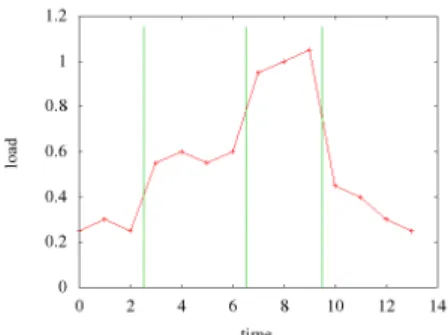
To illustrate the idea, let us assume we only have one metric, the load of the system. Consider a system whose load, measured every second, is displayed in Figure 1; where the x-axis shows the time in seconds and the y-axis the load. With a threshold set to 5%, we can easily recognise 4 phases (following the vertical lines in the graphic, from time 0 to 2, from time 3 to 6, from time 7 to 9, and from time 10 to 13). Each of these phases is characterised by its duration and the different loads the system went through during that phase. The number of phases obviously varies with the threshold, for with a threshold of let’s say 50% we would have had 2 phases (from time 0 to 9, and from time 10 to 13).
As a general rule, a single metric (the load of the system in our example) is not adequate for characterising useful
Figure 1. Example of phase characterization based on load
phases. The set of data chosen will be small enough to save space, but adequately large so as to distinguish between different phases.
As stated beforehand, each phase is associated with its duration and data collected during the phase. The size of the data representing a phase is proportional to its duration, which implies that large amounts of data might be collected for very long phases. To prevent this, a digest is used to summarise the data. We define a signature as a representative for a phase, where the signature is computed from multiple values. In the following, the signature will be computed as the vector of averaged monitored values. In the previous example, the signature of a phase can be the average load during the phase.
C. Phase Identification and Partial Recognition
1) Execution Vectors: In order to apply any of the green
capabilities, it is worth detecting and identifying appropriate phases. An Execution Vector (EV) is a vector of values that represent the behaviour of an application during a time interval. The length of these intervals is defined depending on the goal reactivity. It can be of the order of the mean time to perform an action (switching on or off a node is an action that takes minutes, whereas changing a processor’s frequency is at the second time-scale). EVs are considered as points in the positive quadrant of the execution space spanned by the N vector dimensions; and their values must give a maximum insight on the current execution. These values can be taken from the system (load, network- or I/O-related) or directly from the hardware using performance counters. Hardware performance counters are special hard-ware registers originally designed to performance tuning. However, they have recently been used for investigating the power usage of applications [8], [9]. According to the literature, the most important counters are bus cycles, number of instructions, cache misses, cache hits, cache references, and stall cycles (they may have different names depending on the architecture).
2) Phase Detection and Identification: Following the
0 100 200 300 400 500 600 0 100 200 300 400 500 600
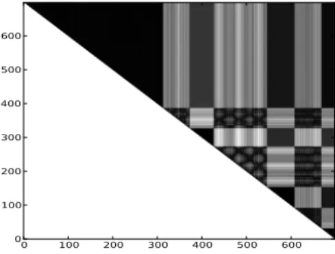
Figure 2. Matrix of distance (manhattan) between execution vectors, where the diagonal represent the execution time line. The darker, the more similar.
loss of generality that during a phase execution vectors are stable.
Figure 2 displays the similarity matrix using execution vectors collected when a cluster was running a synthetic benchmark which successively runs Lower-Upper symmetric Gauss-Seidel (LU), Embarrassingly Parallel (EP), Conjugate Gradient (CG) and Integer Sort (IS) from NPB-3.3 [10] benchmark. A detailed explanation of similarity matrices using power vectors can be found in the literature [11]. As for power vectors, they represent for the whole execution the distance between all pairs of EVs. At coordinate i, j in the upper matrix of Figure 2 the colour represents on a grey scale the distance between the EV at time i and j respectively.
Consequently, the colour at the point i, j tends to black when the distance between EV at i and EV at j tends to zero. Similarly, the colour at the position i, j tends to white as the distance between EV at i and EV at j increases. Above the diagonal line (the diagonal represents the execution timeline from the upper left corner to the lower right corner), we can report 7 triangular blocs. These blocs represent phases the system went through when executing the workload (our synthetic benchmark). From Figure 2, we can also observe that distances between execution vectors within the same phase approach zero, whereas in between phases the distances approach one.
The above observations led us to the premise that a phase change occurs when the distance between two consecutive EVs goes beyond a given threshold, which we refer to as the detection threshold.
While phase detection can serve any kind of system optimisation, keeping all execution vectors is not realistic. Hence, once a phase completes, it is associated a signature vector. The signature vector of a phase is a vector obtained by computing the arithmetic average of each metric (e.g., load, network, or a particular performance counter) of the vectors computed during the phase. It is used for phase identification, where a phase is considered similar to another
if the distance between their signature vectors is below the detection threshold. If the distance between the signature vectors of the new phase and an already identified phase is below the detection threshold, then we do nothing; otherwise a new phase is added via its signature vector to the signature vectors list. Put simply, only the first occurrence of a phase is stored.
3) Partial Recognition: Partial recognition technique is
used to identify phases before their completion. Once a phase is completed, in addition to its signature vector and its characteristics, we store its reference vector and its length. The reference vector of a phase is a randomly chosen execution vector among those pertaining to the set of vectors sampled during the phase. Thus, an ongoing phase (a phase
started but not completed yet) Pongoing is recognised as an
existing phase Pexistif the manhattan distance between each
execution vector of the already executed part of Pongoing
and the reference vector of Pexistis below a given threshold
defining the percentage of dissimilarity between them. We state that the recognition threshold is X% if the already
executed part of Pongoingequals X% of the length of Pexist.
D. Using Phases to Save Energy
Having identified a phase based on information of a previously characterised phase, data on the latter is used for choosing the most relevant green capabilities. The following explains how this approach can be enforced in a distributed system with multiple nodes.
1) Link Between Phases and State: The stability of
met-rics within a phase implies that the behaviour of the system in a phase is more or less constant; meaning that there is a predominant behaviour within the phase. That predominant
behaviouris considered as the state of the phase. Referring
to the literature, a phase can be cpu-intensive, memory-intensive, and IO-intensive (including network accesses).
To find out the predominant behaviour of a phase or its state, we apply Principal Component Analysis (PCA) to the dataset made up by execution vectors belonging to the corresponding phase. PCA is typically issued when several underlying factors shape the data. Therefore, we use variables (each variable represents a metric) contributing less to the first principal axis of PCA to determine the predominant behaviour over the phase (components of the execution vector are access rate of our sensor set).
2) Enforcing Green Leverage: The goal is to optimise the
energy consumption of HPC systems under the following constraints: (a) energy optimisation must be done without any specific information about the characteristics of the application prior to its execution; (b) management policies for reducing the overall system energy consumption must not have a significant impact on performance.
Given these constraints, the most suitable capabilities have to be selected for each phase. Knowing the state of a phase and its remaining time before completion, system adaptation
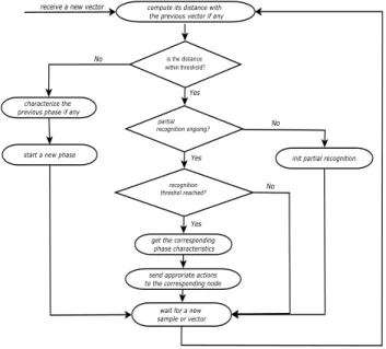
Figure 3. Decision process.
is straightforward via green capabilities. Possible system adaptations are listed bellow.
• Adjusting the system’s computational level: (a) high
or CPU-bound; (b) medium or memory-bound; (c) low for non-CPU/memory-bound applications and idle systems.
• Adjusting the network: (a) interconnects speed; (b)
switching off interconnect equipments.
• Storage/disk availability: (a) switching off memory
banks; (b) spinning down disks.
• Task migration: migrating all tasks to a few nodes can
cut down the energy usage if the rest of the nodes are switched off.
3) Global Architecture: The diagram of Figure 3 shows
the steps of our detection making process. Partial recog-nition starts as soon as a new phase has begun. When the partial recognition threshold is reached (the ongoing phase is identified with an existing phase), the characteristics (including its duration) of the existing phase are used to adapt the system accordingly. In a distributed system with independent nodes we propose a centralised architecture with a global coordinator. The motivation for the centralised management is that task migration, which is one of our green capabilities, requires a global view of the system. Figure 4 depicts the global architecture. The decision making node implements the decision making process; it sends commands to appropriate nodes after decision making. On each node of the system a process samples one execution vector per second and sends it to the global coordinator.
Figure 4. Global coordinator overview.
IV. EXPERIMENTATION ANDVALIDATION
A. Phase Detection and Partial Recognition Results
1) Phase Detection Results: Phase detection is critical
to any management policy that intends to take advantage of workload variability. Analysis of phase detection using power vectors [11] and basic bloc vectors [12] have been provided in the literature. However, these techniques use offline phase analysis. We rely on EVs which are compa-rable to power vectors [11] used in power phase behaviour identification.
The execution vector represents the access rate of a set of performance counters along with the disk access rate (read/write) and network access rate (send/receive) per sec-ond. Each new EV is normalised with respect to a maximum vector. The maximum vector is special in the sense that it comprises the maximum available value of the elements of all execution vectors.
For phase detection, we use the manhattan distance be-tween two consecutive execution points; we then state that two executive EVs belong to the same phase or have the same behaviour if the manhattan distance between them is below a given threshold. The threshold is actually a fixed percentage of the maximum known distance between all consecutive EVs. This maximum is updated any time a greater value is found. Our experiments show that a threshold of 5% is effective in many cases. Figure 5 where doted vertical lines represent the identified phases shows the results of our online phase detection with a 5% threshold on one node of our cluster. During the experiment, our cluster was running the Advance Weather Research and Forecasting (WRF-ARW) [13] model. WRF-AWR is globally one phase broken up with very short transition phases. However, as our phase detection process looks at the runtime behaviour (via execution vectors) of each node of the platform and considers as a phase any behaviour between two consecutive behavioural changes, transition phases will cause WRF-AWR to break into many micro-phases.
To demonstrate the effectiveness of our online detec-tion approach, we implemented using execudetec-tion vectors, the offline phase detection approach presented by Isci et
0 0.1 0.2 0.3 0.4 0.5 0.6 0.7 0.8 0.9 1 0 100 200 300 400 500 600 Normalized rate Time (s) cache-write-op cache-read-op netsentbytes instructions
Figure 5. Online phase detection with a 5% threshold for WRF-ARW.
0 0.1 0.2 0.3 0.4 0.5 0.6 0.7 0.8 0.9 1 0 100 200 300 400 500 600 Normalized rate Time (s) cache-write-op cache-read-op netsentbytes instructions
Figure 6. Online phase detection (with a 5% threshold) and partial recognition (with a 10% threshold) on one of the node running WRF-ARW.
al. [11] on the dataset used for online phase detection.
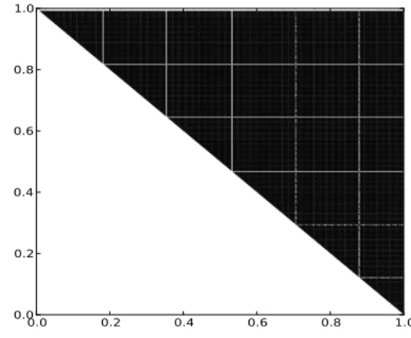
Figure 7 displays in a grey scale the upper diagonal matrix of distances between all pairs of execution vectors. Execution vectors are grouped considering an empirical threshold of 5%, which means that the colour at the position i,j in the graphic tends to white when the manhattan distance between execution vectors at i and j is greater than 5% of the maximum existing distance. Following the phase detection methodology described in Section III-C2; it can be seen from Figure 7 that our online phase detection is as effective as the offline approach.
2) Partial Phase Recognition: We assign to each newly
identified phase a reference vector that is further used for partial phase identification employing the algorithm described in Section III-C. The reference vector is a random vector chosen from the set of vectors belonging to the phase. In Figure 6, similar phases are represented by rectangles filled with the same pattern. For clarity, phases that were partially identified (or identified using partial recognition) start with a small rectangle filled in in black. The length of the rectangle filled in black represents the part of the phase that was used for partial recognition. For this experiment, the recognition threshold was set to an empirical value of 10%. 0.0 0.2 0.4 0.6 0.8 1.0 0.0 0.2 0.4 0.6 0.8 1.0
Figure 7. Offline phase detection with a 5% threshold for WRF-ARW (the matrix corresponds to half of the execution time). The diagonal represents the execution time-line from the upper left corner to the lower right corner.
B. Real-life System Implementation: Measurement and Evaluation Platform
We implemented our online phase detection and recog-nition and tested them on a cluster system. The imple-mented prototype monitors the overall cluster’s behaviour via performance monitoring counters along with network bytes sent/received counts and disk read/write counts. For convenience, we use the term “sensors” to designate per-formance monitoring counters along with network bytes sent/received counts and disk read/write counts. Each node of the cluster sends a sample of data to the decision making node on a per-second basis. Samples collected corresponding to execution vectors are further used by the decision maker node to perform phase detection and partial recognition for any individual node. Partial recognition is more suitable in our case because phases are not detected at fixed intervals; besides, the system may be shared by many applications.
The use of green capabilities available on the managed cluster is guided by our partial phase recognition. When partial recognition is successful, the characteristics of the phase the newly started phase is identified with are trans-lated into a predefined set of “green settings”. The system adaptation implemented so far uses CPU frequency scaling as a proof of concept, but we plan to implement many other green leverages/capabilities including task migration, disk sleep state, and network interconnect speed scaling.
1) Dynamic Power Management via Green
Lever-age/Capabilities: Our phase characterisation relies on the
assumption that sensors contributing less to the first principal axis of PCA give more information about what did not happen during the phase. Thus we arbitrarily select 5 sensors among those contributing less to the first principal axis of PCA for phase characterisation. In addition, we compute
Table I
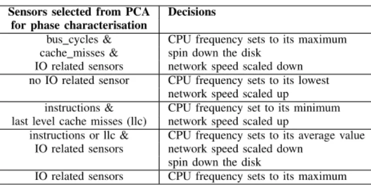
TRANSLATION OF PHASE TO GREEN SETTINGS(IORELATED SENSORS INCLUDES NETWORK AND DISK ACTIVITIES).
Sensors selected from PCA Decisions for phase characterisation
bus cycles & CPU frequency sets to its maximum cache misses & spin down the disk
IO related sensors network speed scaled down no IO related sensor CPU frequency sets to its lowest
network speed scaled up
instructions & CPU frequency set to its minimum last level cache misses (llc) network speed scaled up
instructions or llc & CPU frequency sets to its average value IO related sensors network speed scaled down
spin down the disk
IO related sensors CPU frequency sets to its maximum
the average instruction rate of each phase, which is then used for idle phase characterisation. We need such a metric for characterising idle phases as over the course of idle phases almost all sensors are likely to be constant. Table I shows an example of phases translation to green settings. The left column specifies sensors appearing in the set of sensors selected for phase characterisation; whereas, the right column specifies the associated decision. For instance, when sensors selected from PCA for phase characterisation only include I/O related sensors, the decision associated is scaling the CPU frequency to its maximum.
2) Evaluation Platform: Our evaluation platform is a
fifteen-node cluster set up on the French large-scale
exper-imental platform called Grid50003. Each node is an Intel
Xeon X3440 with 4 cores and 16 GB of RAM. Available frequency steps for each core are: 2.53 GHz, 2.40 GHz, 2.27 GHz, 2.13 GHz, 2.00 GHz, 1.87 GHz, 1.73 GHz, 1.60 GHz, 1.47 GHz, 1.33 GHz and 1.20 GHz. In our experiments, low computational level always sets the CPU frequency to the lowest available frequency, which is 1.20 GHz, whereas high and medium computational levels set the CPU frequency to the highest available (2.53 GHz) and 2.00 GHz respectively. Each node uses its own hard drive which supports active, ready and standby states. Infiniband-20G is used for interconnecting nodes. The Linux kernel 2.6.35 is installed on each node where perf event is used to read the hardware monitoring counters. MPICH is used as MPI library. LU, SP, BT from NPB-3.3 [10] and a real life application the Advance Research WFR (WRF-ARW) model are used for the experiments. Class C of the NAS benchmark is used (compiled with default options). WRF-ARW is a fully compressible conservative-form non-hydrostatic atmospheric model. It uses an explicit time-splitting integration technique to efficiently integrate the Euler equation. We monitored each node power usage on a per second basis using a power distribution unit.
3http://www.grid5000.fr 0 % 20 % 40 % 60 % 80 % 100 % WRF-ARW BT SP LU
Normalized energy consumption
performance phase-detect on-demand
Figure 8. Phase detection and partial recognition guided leverage results: the chart shows the average energy consumption by applications under the three system’s configurations.
C. Experimental Results: Analysis and Discussion
To evaluate our management policy, we consider 3 ba-sic configurations of the monitored cluster: (a) on-demand configuration in which the Linux “on-demand” governor is enabled on all the nodes of the cluster; (b) performance configuration where each node’s CPU frequency scaling governor is set to “performance”; (c) phase-detect config-uration in which we detect phases identified using partial recognition and apply green capabilities accordingly.
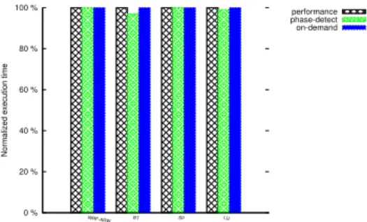
Histograms of Figure 8 present the normalised average energy consumption of the overall cluster for each applica-tion under the three cluster configuraapplica-tions. Figure 9 shows their respective execution time. These figures show that our management policy (phase-detect) consumes in average 15% less energy than “performance” and “on-demand” while offering the same performance for our real-life application, WRF-ARW. For LU, BT and SP the average energy gain is between 3% and 6%, as we could not achieve as much energy savings as with WRF-AWR since many phases detected for these applications are compute intensive. From Figure 9, we notice a performance loss of less than 3% for LU and BT (performance is evaluated in terms of execution time). No need to mention that “on-demand” performs better than “performance” since all the applications we use are CPU intensive. Hence, the CPU load is always above 95% , a situation wherein the on-demand governor remains at the highest frequency.
We do better than a Linux governor because Linux on-demand governor will not scale the CPU frequency down unless the system load decreases below a threshold. The problem at this point is that the CPU load generally remains very high for memory intensive workloads/phases that do not require the full computational power. Thus, the energy gain made with these applications and particularly with WRF-AWR results in slowing the CPU frequency down when a node is suspected to be in a memory-bound phase.
Above results demonstrate the effectiveness of our sys-tem’s energy management scheme based on phase detection and partial recognition. However, there are several underly-ing issues that need to be addressed in the future. Some of
0 % 20 % 40 % 60 % 80 % 100 % WRF-ARW BT SP LU
Normalized execution time
performance phase-detect on-demand
Figure 9. Phase detection and partial recognition guided green leverage results: the chart shows average performance loss incurred by our manage-ment policy with respect to “performance” and “on-demand”.
these issues are highlighted in this paragraph. Performance counters are not the same on all architectures, which means one may need to find out which sensors are useful on his architecture. Despite this limitation, the system management scheme we introduce here is a general purpose model and can be easily scaled to integrate previous research efforts.
V. CONCLUSION
In this paper, we present an approach to optimise the energy consumed by high performance computing systems at runtime. We propose to detect phases of an HPC system based on its workload. Then, by using a partial phase recognition technique, we predict the green capabilities than should be applied to save energy. This detection and improvements are achieved during runtime without knowing any details about the application. A software prototype has been implemented and validated. Experimental results reveal the effectiveness of our phase detection approach under real-life workload and benchmarks. Comparison with baseline unmanaged execution shows that our partial phase recognition algorithm can guide the use of green capabilities and save up to 15% of energy with less than 1% performance degradation. Future work includes integrating workload con-solidation along with task migration as core functionalities of our prototype.
ACKNOWLEDGMENT
This work is supported by the INRIA large scale initiative Hemera focused on “developing large scale parallel and distributed experiments”. Some experiments of this article were performed on the Grid5000 platform, an initiative from the French Ministry of Research through the ACI GRID in-centive action, INRIA, CNRS and RENATER and other con-tributing partners (http://www.grid5000.fr). Authors would also like to thank Marcos Dias de Asuncao for his help in improving the readability of this paper.
REFERENCES
[1] Rountree B, Lowenthal D, Supinski B, Schulz M, Freeh V, Bletsch T, “Adagio: making DVS practical for complex HPC applications,” Proceedings of the 23th International Conference
on Supercomputing (ICS09), Yorktown Heights, New York, USA. 812 Jun., 2009, pp. 460-469.
[2] Kappiah N, Freeh V, Lowenthal D, “Just in time dynamic volt-age scaling: exploiting inter-node slack to save energy in mpi programs,” Proceedings of the 19th ACM/IEEE Conference on Supercomputing (SC05), Washington, USA. 12-18 Nov., 2005, pp. 33-41.
[3] R. Kotla, A. Devgan, S. Ghiasi, T. Keller and F. Rawson, “Characterizing the Impact of Different Memory-Intensity Lev-els,” IEEE 7th Annual Workshop on Workload Characterization (WWC-7), Oct. 2004.
[4] C. Isci, G. Contreras, and M. Martonosi, “Live, runtime phase monitoring and prediction on real systems with application to dynamic power management,” Proc. MICRO, 2006, pp. 359370.
[5] K. Choi, R. Soma, and M. Pedram, “Fine-grained dynamic voltage and frequency scaling for precise energy and perfor-mance tradeoff based on the ratio of off-chip access to on-chip computation times,” IEEE Trans. Comput.-Aided Design Integr. Circuits Syst., vol. 24, no. 1, pp. 1828, Jan. 2005. [6] Lim M, Freeh V, Lowenthal D, “Adaptive, transparent
fre-quency and voltage scaling of communication phases in mpi programs,” in proceedings of the 20th ACM/IEEE Conference on Supercomputing (SC06), Tampa, Florida, USA. 11-17 Nov., 2006, pp. 14-27.
[7] G.L. Tsafack, L. Lefevre, J.M. Pierson, P. Stolf, and G.D. Costa, “DNA-inspired Scheme for Building the Energy Profile of HPC Systems,” In proceedings of the First Inter-national Workshop on Energy-Efficient Data Centres, Madrid, Spain, May 2012.
[8] G. Contreras, “Power prediction for intel xscale processors using performance moni- toring unit events,” In proceedings of the International symposium on Low power electronics and design (ISLPED, ACM Press, 2005, pp. 221226.
[9] K. Singh, M. Bhadauria, and S. A. McKee, “Real time power estimation and thread scheduling via performance counters,” SIGARCH Comput. Archit. News, 37:4655, July 2009.
[10] D. H. Bailey, E. Barszcz, J. T. Barton, R. L. Carter,
T .A. Lasinski, D. S. Browning, L. Dagum, R. A. Fatoohi, P. O. Frederickson, and R. S. Schreiber, “The nas parallel bench-marks. International Journal of High Performance Computing Applications,” 1991, 5:6373.
[11] C. Isci and M. Martonosi. Identifying program power phase behavior using power vectors, “In Workshop on Workload Characterization,” September 2003.
[12] T. Sherwood, E. Perelman, G. Hamerly and B. Calder, “Automatically Characterizing Large Scale Program Behavior,” Proceedings of the Tenth International Conference on Archi-tectural Support for Programming Languages and Operating Systems (ASPLOS X) , Oct., 2002, pp 45-57.
[13] W. C. Skamarock, J. B. Klemp, J. Dudhia, D. Gill, D. Barker, W. Wang, J. G. Powers, “A description of the Advanced Research WRF Version 2. NCAR Technical Note,” NCAR/TN-468+STR (2005).