OATAO is an open access repository that collects the work of Toulouse
researchers and makes it freely available over the web where possible
Any correspondence concerning this service should be sent
to the repository administrator:
[email protected]
This is an author’s version published in: http://oatao.univ-toulouse.fr/25476
To cite this version:
Huang, Jia and Pastor, Marie-Laetitia and Garnier, Christian
and Gong, Xiao-Jing A new model for fatigue life prediction
based on infrared thermography and degradation process for
CFRP composite laminates. (2018) International Journal of
Fatigue, 120. 87-95. ISSN 0142-1123
Official URL:
https://doi.org/10.1016/j.ijfatigue.2018.11.002
A new model for fatigue life prediction based on infrared thermography and
degradation process for CFRP composite laminates
J. Huang
a,b, M.L. Pastor
a,⁎, C. Garnier
b, X.J. Gong
aaInstitut Clément Ader (ICA), CNRS UMR 5312, University of Toulouse, UPS, 1 rue Lautréamont, 65016 Tarbes, France bLGP-ENIT-INP, University of Toulouse, 47 Avenue d’Azereix, BP 1629, 65016 Tarbes cedex, France
Keywords:
Fatigue life prediction InfraRed Thermography (IRT) Damage accumulation Stiffness degradation
A B S T R A C T
In this paper, a new fatigue life prediction methodology is proposed by combining stiffness degradation and temperature variation measured by InfraRed Thermographic (IRT) camera. Firstly, the improved thermographic method is used to determine the fatigue limit by using the data of stabilized temperature rising. Following this, a two-parameter model is proposed to characterize the stiffness degradation of CFRP laminates with the increase of cycle numbers. After the calibration parameters and the calculation of the normalized failure threshold stiffness, the whole −S Ncurve can be obtained in a very short time. The proposed model is applied to both the experimental data of triaxially braided CFRP laminates from literature and those of unidirectional CFRP lami-nates obtained from our fatigue tests. Results show that predictedS−Ncurves have a good agreement with traditional tests. The principal interests of this model could be listed as follows: (i) it is a more general criterion applicable to different materials; (ii) it has more physical senses; (iii) it allows the determination of the total S-N curve for composite materials in a short time.
1. Introduction
Carbon Fiber Reinforced Polymer (CFRP) composites are increas-ingly used to manufacture load-bearing components in aerospace, au-tomotive and marine industries due to their high strength-to-weight
ratio and high stiffness-to-weight ratio. Recently, fatigue properties of
CFRP received more and more concerns since the strength and stiffness of CFRP structural components degrade severely when subjected to
cyclic loading during in-service life, which inevitably affects their
safety. Consequently, a growing number of researchers have been working on the fatigue behavior of composites. Generally speaking,
fatigue limit and stress-life ( −S N) curves are mostly used to
char-acterize fatigue properties. Nevertheless, it is well known that even for
a metallic material, the measurement of one fatigue limit andS−N
curve is time-consuming and costly by conducting traditional fatigue tests. Besides, the fatigue properties of the same material can be dif-ferent due to various loading frequencies, stress ratios, surface
rough-ness values and manufacturing processes[1–4]. Moreover, CFRP
com-posites are more complicated than metals because of their anisotropy and heterogeneity, their fatigue behavior varies also with the nature of fibers and matrix, the volume fraction of fibers, the fiber/matrix
in-terface quality and wide variety offiber orientations and stacking
se-quence, etc. Therefore, rapid evaluation of fatigue behavior for CFRP
composites is of great importance, especially for lightweight structural design. In order to achieve this goal, one of the main ideas is to acquire more information about the response of material subjected to cyclic loading in a short time.
A number of Non-Destructive Evaluation (NDE) methods, such as
radiography [5–7], acoustic emission [8–11] and infrared
thermo-graphy[12–17]have been employed to in situ monitor and characterize
damage evolution within metals and composites under cyclic loading. Among these methods, infrared thermography is advantageous for its real-time and non-contact measurement during fatigue tests. Thus, this
NDE technique has been developed originally by Luong[18,19],
Risi-tano [20,21]and their co-workers as a valid approach to determine
fatigue limit andS−N curve for metallic materials in a short time
(normally around 10 h). Meanwhile, many other criteria based on
thermographic data analysis were proposed to determineS−Ncurve
rapidly[22–28]. However, those criteria, which are developed based on
metal alloys, may not be accurate anymore for composite laminates
because their damage and failure mechanisms are different and even
more complicated. Furthermore, those criteria are almost purely em-pirical formulas which do not take into account damage accumulation process within materials.
The damage mechanism in composite laminates under cyclic loading has been identified usually including matrix cracking, fiber/ ⁎Corresponding author.
E-mail address: [email protected](M.L. Pastor).
matrix interface cracking,fiber breakage and delamination [29].
Ac-cording to the literature[30–36], with damage accumulation in
lami-nates, the stiffness and strength degrade obviously. Thus, residual
stiffness and strength are frequently used to define damage parameters.
Nevertheless, residual strength cannot be evaluated by non-destructive techniques, whereas residual stiffness can be monitored
non-destruc-tively and even in real-time during service life[13,37,38]. Therefore,
stiffness degradation is a preferable parameter to characterize damage
development in a component under cyclic loading. Remarkably, the
work of Toubal[12]shows that this damage accumulation process has a
strong dependence of the evolution of temperature measured by IRT, so the traditional empirical criteria based on IRT can be explained or even improved by introducing damage accumulation analysis.
In the present paper, a new fatigue life prediction model for com-posites materials is proposed by combining IRT data and damage ac-cumulation process. Firstly, the improved thermographic method
pro-posed recently[39]is used here to obtain fatigue limit rapidly. Then, a
curve fitting method is used to estimate the value of the stiffness
threshold under the load corresponding to the fatigue limit. After that, the fatigue damage index of composite materials is established based on
stiffness degradation. Following this, a two-parameter model is
devel-oped to characterize stiffness degradation as a function of the number of cycles performed under different maximum loading stresses. After
parameter calibration with the experimental stiffness degradation and
IRT data, the fatigue damage accumulation model is obtained and can
be used to predict theS−Ncurve. Lastly, the experimental data from
reference[13]as well as our fatigue testing data of CFRP laminates [0]8
are used to validate the proposed model. 2. Background of IRT technique
Generally, fatigue behavior can be considered as an irreversible process of the degradation of mechanical properties under cyclic loading. There are two main approaches in this irreversible process
[19]: (i) a chemical-physical process, such as the movement and the
creation of dislocation, chemical bond rupture, creep deformation, etc. (ii) a physical separation of the material, such as cracks, cavitations, etc. Both of those two approaches will cause heat release which is called intrinsic dissipation. By using an infrared thermographic camera, the variation of temperature can be measured with high precision. A local
heat conduction equation[40–42]can be employed here to explain the
thermodynamic mechanism above:
− = + + +
ρCṪ div( grad )k T di sthe sic re (1)
where ρ, C, T, k are mass density, heat capacity, temperature and heat conduction coefficient, respectively. The first term ρCṪ on the left side
is the heat storage rate due to temperature change, and the second
left-hand term −div( grad ) characterizes heat loss rate induced by con-k T
duction. The term group on the right side represents the different heat
sources:didenotes the intrinsic dissipation source; sthe is the
thermo-elastic source; sic describes the heat source induced by the coupling
effect between internal variables and temperature; andredenotes the
external heat supply. When components or specimens are under homogeneous uniaxial loading, we can have the following hypothesis: (1) Parameters ρ, C, k are material constants and independent of the
internal states.
(2) Thermoelastic sourcesthe only causes small fluctuations of
tem-perature but does not contribute to mean temtem-perature rising[39].
(3) Internal coupling source between internal variables and
tempera-ture, sic, can be neglected[43].
(4) External heat supply reis time-independent and can be removed by
using a reference specimen placed nearby.
Based on the hypothesis above, the intrinsic energy dissipationdi
can be identified as the main contributor to the total heat generated.
Particularly, as can be seen from Eq.(1), ifdiremains unchanged, with
the increase of temperature, the heat loss rate, −div( grad ), will alsok T
increase. It can be deduced that when temperature T reaches a certain value, there exists a balance between heat loss and intrinsic energy dissipation. In this situation, the heat storage rate ρCṪ equals to zero so that T will remain stable. This conclusion has been proved by a number of experiments (with constant stress ratios) in the previous works
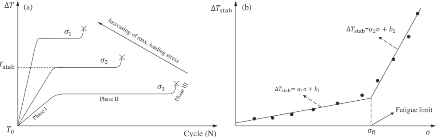
[13,20,21,42,44]. As shown inFig. 1(a), there are three phases from the
beginning of the test to thefinal breakage of the specimen. The
tem-perature increases from an initial value (room temtem-perature) in phase I,
then remains stable for the longest period in phase II andfinally
ex-periences a sharp increase just prior to thefinal breakage in phase III.
Thus, it can be derived thatdikeeps unchanged in phase II, which
in-dicates that the damage accumulation rate is stable in this phase. If different loading stresses are applied, different stabilized temperature
risingΔTstabwill be obtained. Thus, the relationship betweenΔTstaband
σ can be plotted, as shown inFig. 1(b). Based on this, two straight lines are used to characterize the relationship and the intersection can be
considered as the fatigue limit[18,19].
According toFig. 1(b), some empirical criteria were proposed to
predict fatigue life by establishing a direct relationship between
stabi-lized temperature risingΔTstaband failure cycle Nf, such as the criterion
proposed by Risitano[21]:
=
T N
Δstab f constant (2)
and the criterion proposed by Montesano[13]:
Cycle (N)
Phase II=
(a)
(b)
Fatigue limit
Fig. 1. Rapid determination of fatigue limit based on thermographic data. (a) Typical temperature evolution during fatigue test (T0: initial temperature;Δ : tem-T perature rising; TΔstab: stabilized temperature rising; σ : maximum applied loading stress, σ1> σ2> σ3). (b) Fatigue limit determined by an improved method based on statistical analysis.
=
T N
Δ stablog( f) constant (3)
Risitano’s criterion was mainly used to determine the whole fatigue
S-N curves for steels while Montesano’s model was proved to be able to predict S-N curves for braided CFRP laminates. Thus, it can be known
that for different materials, the empirical criteria are not the same. The
reason is that those empirical criteria did not take into account the mechanisms of fatigue damage evolution, which could be distinct for
different materials. Meanwhile, it is still unknown the correlation
be-tween stabilized temperature rising ΔTstab and fatigue damage
accu-mulation speed.
3. Proposed damage accumulation model
3.1. Definition of damage index
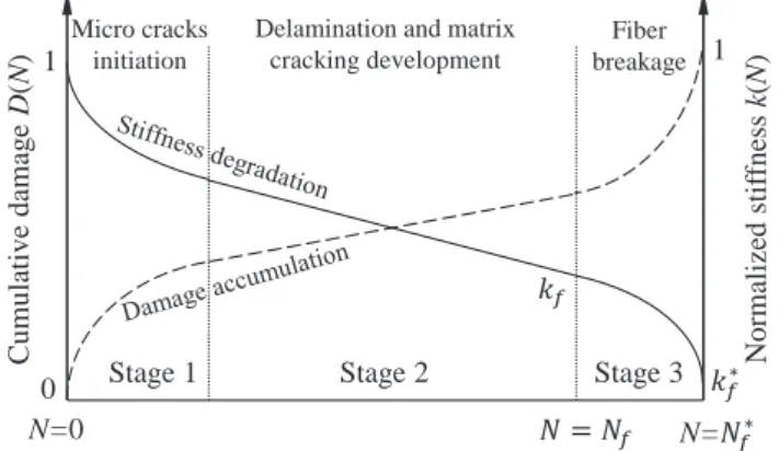
It should be noticed that the main damage mechanisms observed in composites laminates under fatigue loading can also be divided into
three main stages[29,34], as shown inFig. 2. In stage 1, the damage
zone grows rapidly with micro-cracks initiation in the matrix or/and in
thefiber/matrix interface under the first few cycles and some fibers
with low strength may break during this stage. Then the damage ex-periences a slow and steady growth mainly due to delamination and
matrix crack propagation in stage 2. Prior to final failure of the
spe-cimen, the damage grows dramatically with a mass offibers breaking in
stage 3. It is known that stage 3 is short-period (usually less than 1000
cycles) and unstable so that thefirst two stages are usually used to
estimate the residual life of laminates. Similar to the temperature evolution curves, stage 2 with quasi-stable damage growth rate ac-counts for the most parts of the total cycle numbers. Therefore, it can be
deduced that there is a certain relationship betweenΔTstaband the
da-mage accumulation rate. Dada-mage accumulation model based on sti
ff-ness degradation[12]is employed in this work and the fatigue damage
index is defined as follows:
= − − = − − ∗ ∗ ∗ D N K K N K K k N k ( ) ( ) 1 ( ) 1 f f 0 0 (4)
where D* represents cumulative damage level and N is the current
number of loading cycles.K0, K N( )andK∗f are the stiffness of specimen
corresponding to the initial cycle, the Nthcycle and thefinal cycle prior
to failure (also called failure threshold stiffness)N∗
f, respectively.k N( ),
defined as K N K( )/ 0, is normalized stiffness at Nthcycle, andk∗f, defined
as K K∗/
f 0, is normalized failure threshold stiffness at the final cycle.
Similar to damage evolution,k N( )also shows three different stages, as
shown inFig. 2.
In order to propose a practical stiffness degradation model, two
reasonable simplifications are made here. Firstly, only stage 1 and stage
2 are taken into account because stage 3 is a short period where the
damage propagation is unstable and difficult to capture[45,46]. So for
= − − D N k N k ( ) 1 ( ) 1 f (5) 3.2. Proposed model
In order to quantify the damage index, the key is to have the
nor-malized degradation of stiffness as a function of cycle number. As
mentioned before, there is a strong relationship between self-heating response and damage evolution. Therefore, in this work, the normalized stiffness degradation is associated with the stable temperature rise as follows:
= − ≥
k N( ) 1 p TΔ N q(q 1)
stab 1/ (6)
where p and q are two material parameters which are independent of
temperature and loading cycles. In Eq.(6),k N( ) is dimensionless. In
order to keep uniform dimension, the unit of p is in (°C × Cycle1/q)−1
and q is defined as a dimensionless parameter. Those two parameters
can be calibrated by experimental data. The termN1/qcharacterizes the
functional form of normalized stiffness degradation with the increase
cyclic number during stage 1 and stage 2. The role of parameter q is
used to control the shape of the function.ΔTstabvaries as a function of
the applied maximum stress and it is used to describe the general de-gradation speed. The role of parameter p is used to regulate the
influ-ence ofΔTstab, because the scale of temperature response during fatigue
tests depends on the material tested. In the proposed model, the value
of normalized stiffnessk N( ) starts from 1, decreases sharply and then
becomes stable when the cyclic number gets large, which is similar as
experimental normalized stiffness evolution. By combining Eq.(5)and
Eq.(6), the damage index can be expressed as:
= − ≥ D N p T N k q ( ) Δ 1 ( 1) q f stab 1/ (7) After calibration with experimental data for a given material, the
values of p, q and kf can be obtained. In fact,ΔTstab can be also
con-sidered as a bi-linear function of maximum applied stress σ (see
Fig. 1(b)) whose expression is given here:
= = ⎧ ⎨ ⎩ + − ≤ < + ≥ T f σ a σ b b a σ σ a σ b σ σ Δ ( ) ( / ) ( ) stab 1 1 1 1 fl 2 2 fl (8)
wherea1, b1,a2, andb2 denote four empirical constants determined
according to two straight lines in Fig. 1(b) [39]. σfl is the value of
maximum applied loading stress corresponding to fatigue limit[37]. As
well known, the damage index has to equal to unity atfinal or failure
cycle Nf: ifD N( f)=1, we have = − = − ≥ p T N k pf σ N k q 1 Δ 1 ( ) 1 ( 1) f q f f q f stab 1/ 1/ (9)
so the proposed model can predict the wholeS−Ncurve as following:
⎜ ⎟ = ⎛ ⎝ − ⎞ ⎠ ≥ N k pf σ q 1 ( ) ( 1) f f q (10)
Stage 1
Stage 2
Stage 3
Normaliz
ed stif
fne
ss
k(
N
)
N=0
Cumulative damag
e
D
(N
)
0
1
1
Delamination and matrix cracking development Micro cracks initiation Fiber breakage
N=
Fig. 2. Typical damage accumulation and stiffness degradation during fatigue tests.conservative consideration, we define Nf as the number of cycle at the
end of stage 2 and kf as the normalized stiffness degradation atNf
(Fig. 2). Secondly, for a given composite laminate with same stacking
sequence, geometry and fabrication process, if they are subjected to cyclic loading with fixed loading frequency and loading stress ratio, the
critical values of normalized failure threshold stiffness kf∗ can be
con-sidered to be independent of the maximum loading stress level, which
has been proved by previous experimental work [36]. Thus, the kf
corresponding to the end of stage 2 is supposed to be also independent
of the maximum loading stress level. After simplifications, Eq. (5) is
= − = T N k p Δ f q 1 constant f stab 1/ (11)
If q = 1, Eq.(11)turns back to Eq.(2)which is the criterion
pro-posed by Risitano. Moreover, if we change the value of q, the results
obtained from Eq.(11)can be much closer to those from the criterion
proposed by Montesano. An example is given here for explanation. In
fact, by similitude of Eqs.(3)and(11), we can just replace the term
‘N1/q’ in Eq. (6) with‘log( )N ’ to obtain the normalized stiffness
de-gradation model based on Montesano’s criterion:
= −
k N( ) 1 p T'Δ stablog( )N (12)
The experimental stiffness degradation data under the maximum
loading stress of 65% Ultimate Tension Stress (UTS) in[13]have been
used to compare the results of Eqs.(6)and(12), as shown inFig. 3. It
can be seen that the results from the two models have a good
con-cordance. The maximum error of normalized stiffness between two
fitted curves is less than 0.19% from 1 to 104
cycles. Even if the cycle
number is extended to 106, the results from the different functions in
the two models are always pretty close; the maximum error is less than 4.7%. Therefore, it can be concluded that the proposed model is a more
general criterion who can cover both Risitano’s criterion and
Mon-tesano’s criterion.
4. Materials and experimental procedure 4.1. Fabrication of specimens
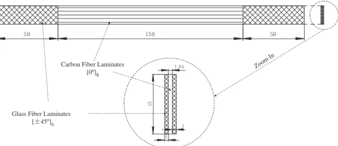
The unidirectional carbon composite specimens used in the present
study was fabricated from carbon prepreg composed of the
HexPly®M79 matrix (epoxy resin) and the 38% UD150/CHS 12 K high
strength carbon fiber. The dimensions of the specimen were as per
standard ISO 527-5:2009 [47]. The nominal cure ply thickness was
given as 0.13 mm, so 8 plies were used to manufacture the UD
com-posite laminates with 1.04 mm nominal thickness, as shown inFig. 4.
The tabs required for gripping were made from glassfiber fabric
pre-preg with epoxy resin and the ply orientation angle was given as ± 45°. Autoclave molding process was employed to cure UD composite lami-nates as well as tabs. The curing of lamilami-nates was performed under
vacuum (−0.9 bar in the vacuum bag). The curing cycle started with
heating up to 80 °C at a heat-up rate of 1 °C/min followed by a 360 min
dwell time and then cooled to room temperature at a rate of−1 °C/
min. Carbonfiber composite laminate was cut into coupons by using
water jet cutting machine and tabs were cut from glassfiber composite
laminate by an abrasive cutter. Hysol EA 9394 Part A + B epoxy resin was used for bonding tabs to coupons in an oven at a temperature of 66 °C for more than 24 h.
4.2. Quasi-static tensile testing
Quasi-static tensile testing was conducted untilfinal breakage of the
specimen in order to determine the ultimate tensile stress (UTS). Experiments were carried out by using Universal Testing Machine (INSTRON 5500R) with digital image correlation technique (DIC) named 3D system Aramis 2 M (GOM, Braunschweig, Germany). The hardware components of DIC system consists of the following parts: (1) two COMS cameras (1624 * 1236 pixels, 8 bits) for image acquisition, (2) a tripod for support and (3) a computer for software installation. Prior to recording, a layer of white paint was applied to the sample
gauge, followed by a layer offinely dispersed black points. According to
standard ISO 527–5:2009, three parallel tests were carried out piloted on the displacement and the actual experimental crosshead velocity was
set as 2.0 mm min−1. The tensile force was recorded by the sensor of
INSTRON 5500R with a scale range of 100 kN and the strainfield was
calculated from the captured images series by using post-processing software of Aramis. Then the modulus of elasticity was determined, based on the data measured above.
4.3. Fatigue testing with IRT camera
In this study, both the traditional approach and the thermographic
approach were used to determine fatigue limit andS−N curve. All
uniaxial fatigue tests were conducted under load-control mode at room temperature by using a servo-hydraulic fatigue testing system (INSTRON MODEL 1342). For each load level, the specimens were subjected to a constant loading amplitude sinusoidal wave-form with a frequency of 5 Hz and a stress ratio of 0.1. An infrared camera (Flir Systems SC7000) with InSb sensors, 320 × 256 pixels, and 20 mK thermal sensitivity was employed here to measure the variation of temperature on the surface of specimens in situ and in real-time. The infrared system is composed of the camera connected to a laptop and
the software called ALTAIR was used for control, configuration and
data post-processing. The detailed experimental setup is shown in
Fig. 5(a). A reference specimen was placed nearby the trial specimen in
order to monitor the temperature change of ambient temperature. The camera was located in front of specimens at a distance of 660 mm in order to record both reference and trial specimen. The spatial resolution
was about 394 × 394μm2. The experimental stiffness K N( ) was
ob-tained from the Nthloop of the measured hysteresis curves by recording
the force and the displacement of the clamp (crossbar of the machine),
Fig. 3. Comparison of the results of stiffness degradation from Eqs.(6)and
(12).
3.3. Principal interests of the proposed model
This model has more physical senses. Unlike pure empirical criteria, this model is established based on the analysis of fatigue damage ac-cumulation process in composites. Fatigue damage is caused by matrix cracking, delamination, and fiber breakage, which produce a large amount of heat and lead to temperature variation. Thus, the stabilized
temperature rising ΔTstab is considered to be an indicator of the speed of
fatigue damage accumulation and the relationship is quantified by Eq.
(7).
The model predict S-N curve in a short time. To obtain stabilized temperature and stiffness degradation curves, it is not necessary to carry out the fatigue tests until the final failure of the specimen. The proposed model can determine S-N curve in 10–12 h, which is sig-nificantly less than the time cost by traditional fatigue testing.
The proposed model is more general. The explanation is given as
as shown inFig. 5(b). Specifically, K N( )was computed as the slope of the line joining the peak and trough of each cycle of the hysteresis
curve. The similar calculation method can be found in[48].
For the traditional fatigue testing approach, several selected max-imum stress (95%, 90%, 85%, 80% and 75% UTS) were applied to
different tests and each test is conducted in load-control until final
failure or over 106 loading cycles. Five specimens were tested under
each maximum loading stress in order to produce a reliable S−N
curve.
For the thermographic testing approach, maximum loading stress level varies from 30% to 90% of UTS at 5% interval in order to obtain the relationship curve between the stabilized rise of temperature and the maximum loading stress. For each maximum loading stress, the specimen was only tested during 6000 loading cycles, which was suf-ficient for recording the stabilized rise of temperature. A total of three specimens were tested for the thermographic testing approach.
5. Validation of the proposed model
In order to validate the proposed model as well as its application range, two cases are carried out using two types of CFRP composite
laminates. For thefirst case, the proposed model is applied to the
ex-perimental data of triaxially braided CFRP laminates presented in[13]
while in the second case, our own experimental data of UD CFRP la-minates is used.
5.1. Case one: triaxially braided CFRP laminates
The experimental data for triaxially braided CFRP laminates used
here have been published in [13], where both thermography and
stiffness degradation data are available. The material tested was carbon
fiber reinforced composite plate which was made from triaxially
braided carbonfiber (T650/35-6 K) fabric with 0°/ ± θ braid
orienta-tion and thermosetting polyamide resin. The fatigue tests were carried
out at a stress ratio of 0.1. In order to show how fatigue limit andS−N
curve are clearly determined, the specific procedure and calibration details are shown step by step as follows:
(1) Determine fatigue limit
In this step, the improved thermographic method three in[39]was
applied here to determine the fatigue limit (Fig. 6). This method is
based on statistical analysis and proved to be an efficient method to
determine the fatigue limit with uniqueness. Fig. 6(a) is a plot of
temperature evolution curve under the maximum loading stress from
30% to 85% of UTS at the interval of 5% UTS.Fig. 6(b) shows the
stabilized temperature rising and the fatigue limit determined is at
67.3% UTS based onFig. 6(a). Since the data are taken from the
re-ference, we cannot carry out experiments to determineΔTstab_fl. So for
this case, the temperature rising of the intersection is taken as TΔstab_fl.
As shown inFig. 6,ΔTstab_flis determined as 6.3 °C.
(2) Determine the values of parameters p and q
50 150 50
1 1.04
1
15
Glass Fiber Laminates
[±45º]6
Carbon Fiber Laminates
[0º]8
Fig. 4. Dimensions of the specimens used in fatigue loading tests.
Infrared Camera Testing Specimen Hydraulic Actuator Reference Specimen (a) 0 2 4 6 8 10 12 14 16 29 29.2 29.4 29.6 29.8 30 30.2 30.4 30.6 N= N= N= N= N= Displacement of clamp (mm) Force (kN) (b)
As mentioned inSection 2, only thefirst two stages are taken into
account. According to the data from the experiments in[13], there are
five different stiffness degradation curves available and only two parameters are necessary. Thus, for each curve, 20 points were
sam-pled, so a total of 100 points are used forfitting. Herein, Eq.(3)is used
tofit the data (3D surface fitting in MATLAB Toolbox) and the values of
parameters p and q can be calibrated. As shown inFig. 7, the
translu-cent surface is the result of surfacefitting by Eq.(3)using MATLAB, and
the values of p and q are determined at 2.42 × 10⁻³(°C × Cycle1/q)−1
and 6.85, respectively.
(3) Calculate the failure threshold stiffness
The failure cycle number Nflcorresponding to fatigue limit is usually
taken between 106and 107[13,41]. Herein, both the k(N =10 )
fl 6 and k
(Nfl=10 )7 are considered to calculate the failure threshold stiffness kf.
According to Eq. (3), for Nfl=106, kf=0.886 is obtained while for
=
Nfl 107,kf=0.841.
(4) Calculate theS−Ncurve
After knowing the values of p, q, and kf, the wholeS−Ncurve can
be plotted according to Eq.(6), and the result is shown inFig. 8.
Tra-ditional test results are also plotted in the samefigure for comparison
(Fig. 8). However, since the experimental data in[13]is limited, the
95% confidence intervals cannot be given.
For triaxially braided CFRP laminates, the predictedS−N curve
corresponding toNfl=107is overall higher than the experimental curve
and the error between predict value and experimental is relatively larger for low fatigue life (less than 10,000 cycles). On the contrary, the
predictedS−N curve corresponding to Nfl=106 is lower than the
traditional test result. Therefore, due to safety reasons,Nfl=106is also
recommended here for engineering applications because the predicted result is more conservative.
5.2. Case two: UD CFRP laminates
The ultimate tensile strength (UTS) and Young’s modulus (E) of the UD CFRP laminates have been measured by carrying out quasi-static
tensile tests with the results of 1487.8 ± 53.2 MPa and
122.6 ± 4.8 GPa, respectively. As mentioned above, the traditional
fatigue tests were performed at least onfive specimens at each
max-imum applied stress, which varied from 75% to 95% UTS with an
in-terval of 5% UTS. The fatigue life values Nf corresponding to each
maximum applied stress were measured so as to establish theS−N
curve presented inFig. 9. The plot is linear on the log-scale from 102
cycles to 106cycles. The data show that the fatigue limit (corresponding
to 106) of the UD composite laminates is in the range of approximately
75–80% UTS and the specific value is estimated to be 75.8% UTS by
using the trend line. For the tests that cycled below fatigue limit, there
were no failure specimens after a run-off of 106
cycles.
Using the same procedure than the case one, the parameter cali-bration steps and the results obtained are listed as below:
Cycle (N) T em p erature rising ( ) Stabili zed tem p erature rising ( )
Maximum loading stress amplitude (UTS%)
(a)
(b)
Stabilized temperature rising corresponding to fatigue limit
Fatigue limit
Fig. 6. Experimental data from[13]. (a) Temperature evolution curves; (b) Fatigue limit determination.
Fig. 7. Surfacefitting of Eq.(3)by MATLAB for triaxially braided CFRP lami-nates. 0% 10% 20% 30% 40% 50% 60% 70% 80% 90% 100% 1000 10000 100000 1000000 10000000 Max imum loading amplitude (UTS) Cycle (N) Experiment Predicted result Predicted result Traditional test result
Fig. 8. Comparison of predicted S-N curves and traditional test results[13]for triaxially braided CFRP laminates.
(1) Determine fatigue limit based on thermographic data
Fig. 10(a) is a plot of the average surface temperature in gauge
section obtained using the IRT camera versus the number of loading cycles for one tested specimen. The maximum stress magnitude is il-lustrated in the plot at the end of each curve. As can be seen in
Fig. 10(a), the temperature profile reached a stabilized plateau at each
maximum loading stress from 30% to 90% of UTS. It should be noticed that the plateau section for 90% UTS is very short because of the
pla-teau section is near to Phase III (seeFigs. 1and2), which is prior to
failure.Fig. 10(b) shows the stabilized temperature rising as a function
of maximum relative load, based on which the fatigue limit can be
determined according to the method described inSection 2. Similarly,
the improved two-curve method [39]isfirstly applied here and the
fatigue limit was determined at 73.8% UTS, which is near to the value (75.8% UTS) determined by traditional tests. Even though the
corre-sponding stabilized temperature rising ( TΔstab_fl) could be determined
by intersection point as shown in Fig. 10(b), the measured value is
preferable to guarantee the quality of the model. Therefore, we have performed additional fatigue tests under maximum stress equal to the measured fatigue limit stress: 73.8% UTS, the stabilized temperature
rising corresponding to fatigue limit ( TΔ stab_fl) was so measured as
0.88 °C ( ± 0.12 °C).
(2) Calibrate the values of parameters p and q
Fig. 11shows the normalized stiffness degradation of tested
speci-mens as a function of cycle number and stabilized temperature rising for the maximum loading stresses of 50%, 60%, 70%, 75% and 80% of
UTS. Thesefive maximum loading stresses were chosen because of the
following reasons: (1) the difference among temperature rising curves for maximum loading stress from 30% to 55% UTS is not great, so only 50% UTS was chosen; (2) 10,000 cycles are needed without reaching an unstable period (phase 3); (3) the chosen maximum loading stresses are preferred to be consistent with case one. Similarly, for each curve, 20
points were sampled and 100 points are used forfitting. Eq.(3)is also
used tofit the data (3D surface fitting in MATLAB Toolbox) and the
values of parameters p and q can be calibrated. The translucent surface
is the result of surfacefitting by Eq.(3)using MATLAB, which is shown
inFig. 11. And the values of p and q are determined as 1.87 × 10⁻²
(°C × Cycle1/q)−1and 4.75, respectively.
(3) Predict the failure threshold stiffness
Similar as previous case, both the k(Nfl=10 )6 and k(Nfl=10 )7 are
considered to calculate the failure threshold stiffness kf. According to
Eq.(3), for Nfl=106,kf= 0.698 is obtained while for Nfl=107, kf=
0.509.
(4) Calculate theS−Ncurve
After knowing the values of p, q, andkf, the wholeS−Ncurve can
be calculated by Eq.(6)and the results are shown inFig. 12. Traditional
test results with the 95% confidence interval are also plotted in the
samefigure for comparison.
As can be seen fromFig. 12, for UD CFRP laminates, the predicted
−
S N curve corresponding toNfl=107 matches well with the
tradi-tional test result for the low and medium fatigue life, whereas the predicted value for high fatigue life (more than 10,000 cycles) is less than the average value of experimental data. The whole predicted
−
S Ncurve is inside the 95% confidence interval. The predicted −S N
curve corresponding toNfl=106is relatively conservative comparing to
experimental results and the predicted fatigue life is less than the
tra-ditional test results overall. For engineering applications,Nfl=106 is
recommended because of safety considerations.
6. Discussions
Based on the study of two cases, it can be found that the predicted −
S N curve corresponding to Nfl=106 is conservative for both two
kinds of CFRP laminates while the predicted S−N curve
70% 75% 80% 85% 90% 95% 100% 100 1000 10000 100000 1000000 Cycle (N) Max imum loading amplitude (UTS) Fatigue limit
Fig. 9.S−N curve determined by traditional fatigue test (R = 0.1 and
f = 5 Hz) of UD CFRP laminates. 0 0.5 1 1.5 2 2.5 3 3.5 4 4.5 0 1000 2000 3000 4000 5000 6000 Cycle (N) 90% UTS 85% UTS 80% UTS 75% UTS
70% UTS 65% UTS60% UTS
55% UTS 50% UTS 45% UTS 40% UTS 35% UTS 30% UTS (a) (b) Stabilized tempera ture rising ( )
Maximum loading stress amplitude (UTS%)
T
emperature rising
(
)
Fatigue limit
Fig. 10. Fatigue limit determination of UD CFRP based on IRT experimental data. (a) Evolution of the temperature rising as a function of loading cycle number for one specimen; (b) Fatigue limit determined by the improved two-curve method.
corresponding toNfl=107overestimated the fatigue life in some cases. It should be also noticed that under same maximum loading level, the
value ofΔTstabof triaxially braided CFRP laminates is much greater than
that of UD CFRP laminates. It may be caused by the different dimension
of the specimen and different amount of heat generated by internal friction. For thicker and wider specimens, there is more heat generation which may lead to higher temperature rising. Also, the heat generated by internal friction effect between fibers and matrix in UD CFRP la-minates could be different. Thus, it is not reasonable to use stabilized temperature rising directly to describe damage evolution. In our pro-posed model, by adjusting the value of parameter p, the damage ac-cumulation rate related to temperature rising can be regulated. As shown in step two of the parameter calibration procedure, the value of p for UD CFRP laminates is almost 8 times the value of p for triaxially braided CFRP laminates, which indicates that the braided CFRP lami-nates produce more heat during fatigue tests, compared to UD CFRP
laminates. That may be because there is much more friction effect in
braided CFRP laminates than in UD CFRP laminates. As for q, the value of parameter q for braided CFRP laminates is greater than UD CFRP
laminates, which means that the stiffness degradation of braided CFRP
laminates is faster than that of UD CFRP laminates. It is sure that more experimental data are necessary to confirm the physical interpretation
of the constants p and q. 7. Conclusions
A practical and quick methodology was proposed to evaluate fatigue life of CFRP laminate in this paper. The damage accumulation process and temperature evolution of composite laminates under fatigue loading were discussed initially to provide theoretical basis. The sta-bilized temperature rising measured with help of an infrared camera is
considered to be able to reflect the rate of damage accumulation. A
two–parameter model was developed based on damage accumulation
process, which combined stabilized temperature rising and normalized
stiffness degradation. It is shown that the proposed model is more
general, it can include some empirical criteria proposed in the literature and has a wider application scope. In order to validate proposed methodology, the experimental data obtained on two different types of CFRP laminates, UD and triaxially braided CFRP laminates, were used in the present work to calibrate the two empirical parameters necessary
for the establishment of the model. Two failure cycles (Nfl=106 and
=
Nfl 107) related to fatigue limit were considered for the determination
of the failure threshold stiffness, and then the whole −S N curve
cor-responding to each failure cycles. Compared to the S-N curve obtained
by the traditional testing method, theS−N curve corresponding to
=
Nfl 107for UD CFRP laminates is inside the 95% confidence intervals,
while the predicted results for triaxially braided CFRP laminates are
higher than experimental data. The S−N curve corresponding to
=
Nfl 106is recommended for both of the two types of composite
ma-terials because the predicted results are relatively more conservative. By comparison of the fatigue life prediction used in the proposed model, the physical sense of each of the two parameters has been discussed. The whole determination process takes about 10–12 h, which is much faster and simpler than traditional fatigue testing method. Therefore, even though the proposed method based on thermographic measure-ment should have to be confirmed by much more experimeasure-mental data, it has shown a very promising way to evaluate rapidly fatigue limit and
−
S N curve for composite laminates, which are considered very
im-portant mechanical properties for engineering application of these materials.
Acknowledgements
The author Jia Huang was supported by the China Scholarship
50% UTS 60% UTS
70% UTS
75% UTS
80% UTS
Fig. 11. Surfacefitting of Eq.(3)by MATLAB for UD CFRP laminates.
0% 10% 20% 30% 40% 50% 60% 70% 80% 90% 100% 100 1000 10000 100000 1000000 Maxim um loading am plitude (U TS) Cycle (N) Experiment P=95% Lower bond Upper bond Predicted result Predicted result Traditional test result
Fig. 12. Comparison of predicted S-N curves and traditional test results for UD CFRP laminates.
[1] Fargione G, Giudice F, Risitano A. The influence of the load frequency on the high cycle fatigue behaviour. Theor Appl Fract Mech 2017;88:97–106.
[2] Mohammadi B, Fazlali B. Off-axis fatigue behaviour of unidirectional laminates based on a microscale fatigue damage model under different stress ratios. Int J Fatigue 2018;106:11–23.
[3] Lopes HP, Elias CN, Vieira MVB, Vieira VTL, de Souza LC, dos Santos AL. Influence of surface roughness on the fatigue life of nickel-titanium rotary endodontic in-struments. J Endod 2016;42(6):965–8.
[4] Bagehorn S, Wehr J, Maier HJ. Application of mechanical surfacefinishing pro-cesses for roughness reduction and fatigue improvement of additively manufactured Ti-6Al-4V parts. Int J Fatigue 2017;102:135–42.
[5] Scott AE, Sinclair I, Spearing SM, Thionnet A, Bunsell AR. Damage accumulation in a carbon/epoxy composite: Comparison between a multiscale model and computed tomography experimental results. Compos A Appl Sci Manuf 2012;43(9):1514–22. [6] Garcea SC, Mavrogordato MN, Scott AE, Sinclair I, Spearing SM. Fatigue
micro-mechanism characterisation in carbonfibre reinforced polymers using synchrotron radiation computed tomography. Compos Sci Technol 2014;99(Supplement C):23–30.
[7] Garcea SC, Sinclair I, Spearing SM. Fibre failure assessment in carbonfibre re-inforced polymers under fatigue loading by synchrotron X-ray computed tomo-graphy. Compos Sci Technol 2016;133(Supplement C):157–64.
[8] Masmoudi S, El Mahi A, Turki S. Fatigue behaviour and structural health mon-itoring by acoustic emission of E-glass/epoxy laminates with piezoelectric implant. Appl Acoust 2016;108:50–8.
[9] Oh KS, Han KS. Fatigue life modeling of shortfiber reinforced metal matrix com-posites using mechanical and acoustic emission responses. J Compos Mater 2013;47(10):1303–10.
[10] Bourchak M, Farrow IR, Bond IP, Rowland CW, Menan F. Acoustic emission energy as a fatigue damage parameter for CFRP composites. Int J Fatigue
2007;29(3):457–70.
[11] Kordatos EZ, Dassios KG, Aggelis DG, Matikas TE. Rapid evaluation of the fatigue limit in composites using infrared lock-in thermography and acoustic emission. Mech Res Commun 2013;54(4):14–20.
[12] Toubal L, Karama M, Lorrain B. Damage evolution and infrared thermography in woven composite laminates under fatigue loading. Int J Fatigue
2006;28(12):1867–72.
[13] Montesano J, Fawaz Z, Bougherara H. Use of infrared thermography to investigate the fatigue behavior of a carbonfiber reinforced polymer composite. Compos Struct 2013;97:76–83.
[14] Palumbo D, De Finis R, Demelio PG, Galietti U. A new rapid thermographic method to assess the fatigue limit in GFRP composites. Compos B Eng 2016;103:60–7. [15] Crupi V, Guglielmino E, Scappaticci L, Risitano G. Fatigue assessment by energy
approach during tensile and fatigue tests on PPGF35. Proc Struct Integrity 2017;3:424–31.
[16] Gao B, He Y, Woo WL, Tian GY, Liu J, Hu Y. Multidimensional tensor-based in-ductive thermography with multiple physicalfields for offshore wind turbine gear inspection. IEEE Trans Ind Electron 2016;63(10):6305–15.
[17] Gao B, Lu P, Woo WL, Tian GY, Zhu Y, Johnston M. Variational bayesian sub-group adaptive sparse component extraction for diagnostic imaging system. IEEE Trans Ind Electron 2018;65(10):8142–52.
[18] Luong MP. Infrared thermographic scanning of fatigue in metals. Nucl Eng Des 1995;158(2):363–76.
[19] Luong MP. Fatigue limit evaluation of metals using an infrared thermographic technique. Mech Mater 1998;28(1):155–63.
[20] La Rosa G, Risitano A. Thermographic methodology for rapid determination of the fatigue limit of materials and mechanical components. Int J Fatigue
2000;22(1):65–73.
[21] Fargione G, Geraci A, La Rosa G, Risitano A. Rapid determination of the fatigue curve by the thermographic method. Int J Fatigue 2002;24(1):11–9.
[22] Huang Y, Li S, Lin S, Shih C. Using the method of infrared sensing for monitoring fatigue process of metals. Materials Evaluation (United States), 42(8); 1984.
[23] Jiang L, Wang H, Liaw P, Brooks C, Klarstrom D. Characterization of the tem-perature evolution during high-cycle fatigue of the ULTIMET superalloy: experi-ment and theoretical modeling. Metall Mater Trans A 2001;32(9):2279–96. [24] Jiang L, Wang H, Liaw P, Brooks C, Chen L, Klarstrom D. Temperature evolution
and life prediction in fatigue of superalloys. Metall Mater Trans A 2004;35(3):839–48.
[25] Yang B, Liaw P, Wang G, Morrison M, Liu C, Buchanan R, et al. In-situ thermo-graphic observation of mechanical damage in bulk-metallic glasses during fatigue and tensile experiments. Intermetallics 2004;12(10):1265–74.
[26] Curà F, Curti G, Sesana R. A new iteration method for the thermographic de-termination of fatigue limit in steels. Int J Fatigue 2005;27(4):453–9.
[27] Amiri M, Khonsari MM. Life prediction of metals undergoing fatigue load based on temperature evolution. Mater Sci Eng, A 2010;527(6):1555–9.
[28] Amiri M, Khonsari MM. Rapid determination of fatigue failure based on tempera-ture evolution: Fully reversed bending load. Int J Fatigue 2010;32(2):382–9. [29] Vasiukov D, Panier S, Hachemi A. Direct method for life prediction offibre
re-inforced polymer composites based on kinematic of damage potential. Int J Fatigue 2015;70:289–96.
[30] Post NL, Lesko JJ, Case SW. 3 - Residual strength fatigue theories for composite materials, fatigue life prediction of composites and composite structures. Woodhead Publishing; 2010. p. 79–101.
[31] Caous D, Bois C, Wahl JC, Palin-Luc T, Valette J. A method to determine composite material residual tensile strength in thefibre direction as a function of the matrix damage state after fatigue loading. Compos Part B: Eng 2017;127(Supplement C):15–25.
[32] Llobet J, Maimí P, Mayugo JA, Essa Y, Martin de la Escalera F. A fatigue damage and residual strength model for unidirectional carbon/epoxy composites under on-axis tension-tension loadings. Int J Fatigue 2017;103(Supplement C):508–15. [33] Stojković N, Folić R, Pasternak H. Mathematical model for the prediction of
strength degradation of composites subjected to constant amplitude fatigue. Int J Fatigue 2017;103(Supplement C):478–87.
[34] Shiri S, Yazdani M, Pourgol-Mohammad M. A fatigue damage accumulation model based on stiffness degradation of composite materials. Mater Des 2015;88:1290–5. [35] Senthilnathan K, Hiremath CP, Naik NK, Guha A, Tewari A. Microstructural damage
dependent stiffness prediction of unidirectional CFRP composite under cyclic loading. Compos Part A: Appl Sci Manuf 2017;100(Supplement C):118–27. [36] Peng T, Liu Y, Saxena A, Goebel K. In-situ fatigue life prognosis for composite
la-minates based on stiffness degradation. Compos Struct 2015;132:155–65. [37] Whitworth HA. A stiffness degradation model for composite laminates under fatigue
loading. Compos Struct 1997;40(2):95–101.
[38] Tang R, Guo YJ, Weitsman YJ. An appropriate stiffness degradation parameter to monitor fatigue damage evolution in composites. Int J Fatigue 2004;26(4):421–7. [39] Huang J, Pastor ML, Garnier C, Gong X. Rapid evaluation of fatigue limit on
ther-mographic data analysis. Int J Fatigue 2017;104(Supplement C):293–301. [40] Boulanger T, Chrysochoos A, Mabru C, Galtier A. Calorimetric analysis of
dis-sipative and thermoelastic effects associated with the fatigue behavior of steels. Int J Fatigue 2004;26(3):221–9.
[41] Chrysochoos A, Dattoma V, Wattrisse B. Deformation and dissipated energies for high cycle fatigue of 2024–T3 aluminium alloy. Theor Appl Fract Mech 2009;52(2):117–21.
[42] Guo Q, Guo X, Fan J, Syed R, Wu C. An energy method for rapid evaluation of high-cycle fatigue parameters based on intrinsic dissipation. Int J Fatigue
2015;80:136–44.
[43] Guo Q, Guo X. Research on high-cycle fatigue behavior of FV520B stainless steel based on intrinsic dissipation. Mater Des 2016;90(Supplement C):248–55. [44] Wang XG, Crupi V, Guo XL, Zhao YG. Quantitative thermographic methodology for
fatigue assessment and stress measurement. Int J Fatigue 2010;32(12):1970–6. [45] Tao C, Ji H, Qiu J, Zhang C, Wang Z, Yao W. Characterization of fatigue damages in
composite laminates using Lamb wave velocity and prediction of residual life. Compos Struct 2017;166:219–28.
[46]Lee LJ, Fu KE, Yang JN. Prediction of fatigue damage and life for composite la-minates under service loading spectra. Compos Sci Technol 1996;56(6):635–48. [47] ISO 527-5:2009, Plastics - Determination of tensile properties - Part 5: Test
condi-tions for unidirectionalfibre-reinforced plastic composites.
[48]Carrillo J, Vargas D, Sánchez M. Stiffness degradation model of thin and lightly reinforced concrete walls for housing. Eng Struct 2018;168:179–90.
Council for 3 years study at the University of Toulouse. References

![Fig. 6. Experimental data from [13] . (a) Temperature evolution curves; (b) Fatigue limit determination.](https://thumb-eu.123doks.com/thumbv2/123doknet/2972270.82687/7.892.78.822.85.350/fig-experimental-temperature-evolution-curves-fatigue-limit-determination.webp)


