HAL Id: tel-02096565
https://tel.archives-ouvertes.fr/tel-02096565
Submitted on 11 Apr 2019HAL is a multi-disciplinary open access
archive for the deposit and dissemination of sci-entific research documents, whether they are pub-lished or not. The documents may come from teaching and research institutions in France or abroad, or from public or private research centers.
L’archive ouverte pluridisciplinaire HAL, est destinée au dépôt et à la diffusion de documents scientifiques de niveau recherche, publiés ou non, émanant des établissements d’enseignement et de recherche français ou étrangers, des laboratoires publics ou privés.
Ahmad Farhat
To cite this version:
Ahmad Farhat. Use of Wireless Sensor Networks for Operational Safety and Industrial Prognosis. Per-formance [cs.PF]. Université Bourgogne Franche-Comté; Université libanaise, 2017. English. �NNT : 2017UBFCD046�. �tel-02096565�
THESE DE DOCTORAT DE L’ETABLISSEMENT UNIVERSITE BOURGOGNE FRANCHE-COMTE
PREPAREE A l'Université LIBANAISE, BOURGOGNE FRANCHE-COMTE
ED SPIM : Sciences pour l'ingénieur et microtechnique.
ED ST: Ecole Doctorale des Sciences et de Technologie
Doctorat
d’Informatique
Par
Ahmad FARHAT
Use of Wireless Sensor Networks for operational safety and industrial prognosis
Thèse présentée et soutenue à Belfort- France le 17/11/2017
Composition du Jury :
Pierre Spiteri Professeur émérite IRIT - ENSEEIHT Président
Pierre Spiteri Professeur émérite IRIT - ENSEEIHT Rapporteur
Haidar Safa Professeur à l’Université Américaine de Beyrouth (AUB), Libanais, Rapporteur Chady Abou JAOUDE Professeur à l’Université Antonine Examinateur Yehia TAHER Université de Versailles Saint-Quentin-En- Yvelines Maître de conférences Examinateur Christophe GUYEUX Professeur à l’Université de Franche-Comté Directeur de thèse Mourad HAKEM Maître de conférences à l’Université de Franche-Comté Codirecteur de thèse Abbas HIJAZI Professeur à l’Université Libanaise Directeur de thèse Ali JABER Maître de conférences à l’Université Libanaise Codirecteur de thèse
Titre : titre (en français) : Utilisation de réseaux de capteurs sans fil pour la sécurité opérationnelle et
le pronostic industriel
Mots clés : Réseaux de capteurs sans fil, Pronostic et gestion de l’état de santé d’un dispositif
industriel, Diagnostic.
Résumé:
Une maintenance efficace d’un dispositif industriel ne peut être basée que sur la fiabilité et l’exactitude de données physiques captées sur ledit dispositif, à des fins de surveillance. Dans certains cas, le monitoring de tels systèmes industriels ou de zones à surveiller ne peut pas être assuré à l’aide de capteurs individuels ou filaires, du fait par exemple de problèmes d’accès ou de milieux hostiles. Les Réseaux de Capteurs Sans Fil (RCSF) sont alors une alternative. En raison de la nature des communications dans ces réseaux, et des caractéristiques des appareils composants ces derniers, un RCSF est à fort risque de pannes au niveau des capteurs, et dans ce cas la perte de diverses données est probable - ce qui peut s’avérer problématique pour le monitoring du dispositif. Pour étudier la pertinence des RCSF pour le processus dit de PHM (Prognostic and Health Management, utilisé pour déterminer le plan de maintenance d’un dispositif à surveiller), et l’impact des diverses stratégies déployées dans ces premiers sur ces derniers, nous avons proposé un premier algorithme de diagnostic efficace et l’avons utilisé dans un RCSF simulé pour en mesurer la performance (ce simulateur étant un programme que nous avons développé).Nous avons alors proposé une démarche pour diagnostiquer l’état de systèmes physiques basée sur l’utilisation de la méthode dite des forêts aléatoires. Cette démarche repose sur deux phases : une première, hors ligne, et une seconde en ligne. Dans la phase hors ligne, l’algorithme des forêts aléatoires sélectionne les paramètres qui contiennent le plus d’information sur l’état du système. Ces paramètres sont utilisés, dans leur ordre d’importance, pour construire les arbres décisionnels qui constitueront la forêt. En injectant de l’aléatoire dans la base d’apprentissage, l’algorithme utilisera divers points de départ, et par la suite les arbres aussi seront aléatoires. Dans la phase en ligne, l’algorithme évalue l’état actuel du système en utilisant les données capteurs pour parcourir les arbres construits. Chaque arbre dans la forêt fournit une décision, et la classe finale est le résultat d’un vote majoritaire sur l’ensemble de la forêt. Quand les capteurs commencent à tomber en panne, certaines données associées à divers indicateurs de santé s’avèrent incomplètes ou sont perdues. Or, puisque les arbres ont des points de départ différents, l’absence de mesures pour un indicateur de santé ne conduit pas nécessairement à l’interruption du processus de prédiction de l’état global de santé du dispositif industriel : le processus de monitoring peut alors continuer.
Title : Titre en anglais) :
Use of Wireless Sensor Networks for operational safety and industrial
prognosis
Keywords : Wireless Sensor Networks, Prognostic and Health Management, Diagnostic.
Abstract :
Efficient maintenance of an industrial device can only be based on the reliability and accuracy of physical data captured on the device for monitoring purposes. In some cases, monitoring of such industrial systems or areas to be monitored cannot be carried out using individual or wired sensors, for example due to access problems or hostile environments. Wireless Sensor Networks (WSN) are then an alternative. Due to the nature of communications in these networks, and the characteristics of the devices that make up these networks, an WSNs is at high risk of sensor failures, and in this case the loss of various data is likely - which can be problematic for device monitoring. To study the relevance of WSNs for the so-called PHM (Prognostic and Health Management process, used to determine the maintenance plan of a device to be monitored), and the impact of the various strategies deployed in the latter, we proposed a first efficient diagnostic algorithm and used it in a simulated WSNs to measure its performance (this simulator being a program we developed).We then proposed an approach to diagnose the condition of physical systems based on the use of the so-called random forest method. This approach is based on two phases: a first phase, offline, and a second phase online. In the offline phase, the random forest algorithm selects the parameters that contain the most information about the system's state. These parameters are used, in order of importance, to construct the decision trees that will make up the forest. By injecting randomness into the learning base, the algorithm will use various starting points, and then the trees too will be random. In the online phase, the algorithm evaluates the current state of the system by using the sensor data to scan the constructed trees. Each tree in the forest provides a decision, and the final class is the result of a majority vote on the whole forest. When the sensors begin to fail, some of the data associated with various health indicators are incomplete or lost. However, since trees have different starting points, the absence of measures for a health indicator does not necessarily lead to the interruption of the process of predicting the overall state of health of the industrial system: the monitoring process can then continue.
Université Bourgogne Franche-Comté 32, avenue de l’Observatoire
Thèse de Doctorat
é c o l e d o c t o r a l e s c i e n c e s p o u r l ’ i n g é n i e u r e t m i c r o t e c h n i q u e s
U N I V E R S I T É D E F R A N C H E - C O M T É
n
Use of Wireless Sensor Networks
for Operational Safety and Industrial
Prognosis
Thèse de Doctorat
é c o l e d o c t o r a l e s c i e n c e s p o u r l ’ i n g é n i e u r e t m i c r o t e c h n i q u e s
U N I V E R S I T É D E F R A N C H E - C O M T É
Use of Wireless Sensor Networks for Operational
Safety and Industrial Prognosis
A dissertation presented by
Ahmad FARHAT
and submitted to the
University of Bourgogne Franche-Comt ´e
in Partial Fulfillment of the Requirements for obtaining the DegreeDOCTOR OF PHILOSOPHY
Speciality:Computer ScienceResearch Unit:
Laboratory of Femto-St (SPIM)
Defended in public on 17 November 2017 in front of the jury composed from:
PIERRESPITERI´ Reviewer Professor at Institut National Polytechnique De
Toulouse (Jury President)
HAIDAR SAFA Reviewer Professor at the American University of Beirut (AUB)
YEHIATAHER Examiner Assistant Professor at the University of Versailles
Saint-Quentin-En-Yvelines
CHADY ABOU JAOUDE Examiner Professor at the Antonine University
CHRISTOPHEGUYEUX Supervisor Professor at University of Bourgogne
Franche-Comt ´e
MOURADHAKEM Co-supervisor Assistant Professor at University of Bourgogne Franche-Comt ´e
ABBASHIJAZI Supervisor Professor at the Lebanese University
ALIJABER Co-supervisor Assistant Professor at the Lebanese University
Table of contents 4 List of figures 7 List of tables 9 List of abbreviations 11 Dedication 13 Acknowledgements 15
I Scientific background and issues 17
1 General introduction 19 1.1 Dissertation Outline . . . 24 1.2 Publications . . . 25 1.2.1 Published papers . . . 25 1.2.2 Submitted papers . . . 25 2 Scientific background 27 2.1 An overview on Wireless Sensor Networks . . . 27
2.1.1 Systems software for WSNs . . . 28
2.1.2 Sensor network applications . . . 31
2.1.2.1 Environmental applications . . . 31
2.1.2.2 Military applications . . . 31
2.1.2.3 Home applications . . . 32
2.1.2.4 Health applications . . . 32
2.1.2.5 Other commercial applications . . . 32
2.1.3 Shortcomings of a WSN . . . 33
2.1.3.1 Resources . . . 33 1
2.1.3.2 Communication . . . 33
2.2 Prognostics and Health Management . . . 34
2.2.1 Data acquisition . . . 35
2.2.2 Data processing . . . 36
2.2.3 Health assessment . . . 36
2.2.4 Diagnostics . . . 37
2.2.5 Prognostics . . . 38
2.2.6 Decision support system . . . 39
2.2.7 Human machine interface . . . 40
2.3 Industrial Prognostics and Health Management by WSNs . . . 40
2.4 The challenges faced . . . 41
2.5 Conclusion . . . 43
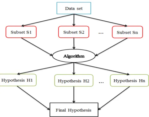
II Contributions 45 3 Diagnosis via the Random Forests Algorithm 47 3.1 Introduction . . . 47 3.2 Related work . . . 49 3.3 Machine learning . . . 49 3.3.1 Reinforcement learning . . . 50 3.3.2 Deep learning . . . 51 3.3.3 Supervised learning . . . 51 3.3.4 Unsupervised learning . . . 51 3.3.5 Semi-supervised learning . . . 52 3.4 Ensemble methods . . . 52 3.5 Overview of diagnostics . . . 53
3.6 The random forests algorithm . . . 55
3.7 Experimental study . . . 59
3.7.1 Data collection . . . 59
3.7.1.1 Set of experiment 1 . . . 59
3.7.1.2 Set of experiment 2 . . . 59
3.7.2 Random forest design . . . 60
3.7.3 Providing a diagnostic on a new set of observations . . . 61
3.7.4 Numerical simulations . . . 62
4 Impact of WSNs strategies on prognostics and health management 65
4.1 Introduction . . . 66
4.2 Coverage issues in Wireless Sensor Networks . . . 67
4.3 Topologies issues in Wireless Sensor Networks . . . 69
4.4 Benefits of WSN in PHM . . . 71
4.4.1 Complete coverage . . . 72
4.4.2 Coverage hole . . . 73
4.4.3 Deployment strategy . . . 73
4.4.4 Coverage algorithms . . . 73
4.4.5 Sensors on long term . . . 73
4.4.6 Density . . . 74
4.4.7 Reliability . . . 74
4.4.8 WSN models . . . 74
4.5 Experimental protocol . . . 74
4.5.1 Wireless sensor network simulation . . . 74
4.5.2 Machine learning algorithms . . . 76
4.6 Simulation results . . . 77
4.6.1 Impact of scheduling mechanism in WSN on diagnostics . . . 77
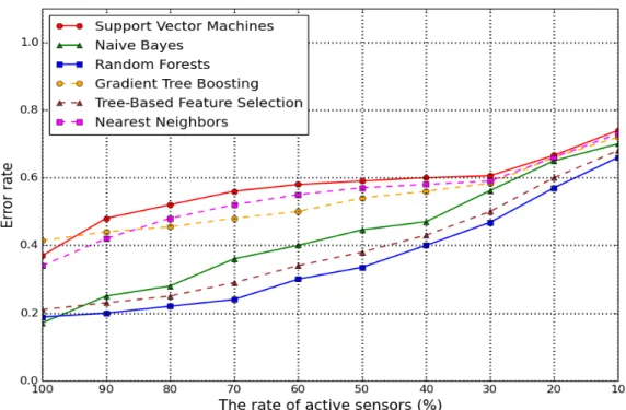
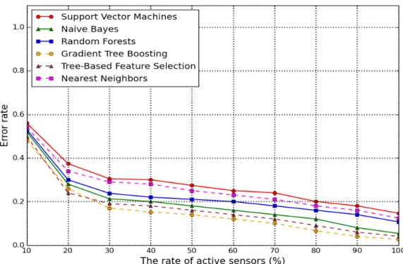
4.6.2 Impact of density-deployment of sensors on diagnostics . . . 81
4.6.3 Impact of topologies on diagnostics . . . 85
4.6.3.1 Decentralized topology . . . 85 4.6.3.2 Distributed topology . . . 89 4.6.3.3 Hierarchical topology . . . 91 4.6.3.4 Centralized topology . . . 95 4.6.3.5 Discussion . . . 96 4.6.4 Algorithm complexities . . . 97 4.7 Conclusion . . . 98
5 Distributed minimal dominating sensor-targets for diagnostics 101 5.1 Introduction . . . 101
5.2 Energy efficiency of coverage protocols in WSN . . . 102
5.3 Probabilistic Coverage Protocol . . . 104
5.4 Dominating sets . . . 105
5.4.1 Simple dominating sets . . . 105
5.4.3 Total dominating sets . . . 106
5.5 The proposed algorithm . . . 107
5.5.1 Correctness and convergence proofs . . . 109
5.6 Simulation results . . . 110
5.6.1 Comparison with the optimistic BaseLine solution . . . 112
5.6.2 Comparison with the PCP algorithm . . . 115
5.7 Conclusion . . . 118
III Conclusion 119 6 Conclusion and Perspectives 121 6.1 Conclusion . . . 121
6.2 Perspectives . . . 123
1.1 Catastrophes due to failure outcomes. . . 20
1.2 History of maintenance strategies. . . 21
1.3 General steps of PHM. . . 22
2.1 Wireless Sensor Networks monitoring. . . 28
2.2 Reference hardware platform architecture of a sensor node. . . 29
2.3 Protocol stack for WSN. . . 30
2.4 Data acquisition system. . . 35
2.5 Data processing system. . . 36
2.6 Health assessment process. . . 37
2.7 Diagnostics different steps. . . 37
2.8 An illustration of RUL with uncertainties. . . 38
2.9 Decision support system. . . 39
2.10 Human machine interaction. . . 40
2.11 PHM steps with WSN monitoring. . . 41
3.1 Machine learning algorithms. . . 50
3.2 Data set diversification in homogeneous ensemble methods. . . 53
3.3 Algorithm diversification in heterogeneous ensemble methods. . . 53
3.4 An illustration of the random forest. . . 56
3.5 Example of a tree in the random forest. . . 61
3.6 Delay in failure detection with respect to the number of simulations. . . 62
3.7 Error rate in diagnostics with respect to the number of simulations. . . 63
3.8 Number of successful diagnostics with respect to the number of trees. . . . 63
4.1 Types of coverage problems. . . 69
4.2 PHM steps with insufficient coverage in WSN. . . 71
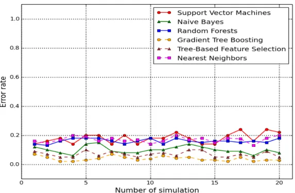
4.3 Error rate in diagnostics in the case of complete learning and the percent-age of active sensors is 100 % with respect to the number of simulations. . 78 4.4 Error rate in diagnostics in the case of incomplete learning and the
per-centage of active sensors is 100 % with respect to the number of simulations. 79 5
4.5 Error rate in diagnostics in case of complete learning with the variation of
the percentage of active sensors. . . 80
4.6 Error rate in diagnostics in case of incomplete learning with the variation of the percentage of active sensors. . . 81
4.7 Error rate in diagnostics in the case of complete learning with respect to the number of simulations. . . 82
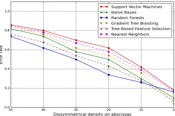
4.8 asymmetrical density on abscissa. . . 83
4.9 Error rate in diagnostics with the variation of data learning in a way of asymmetrical density on the abscissas (length of area monitoring). . . 83
4.10 Error rate in diagnostics with the variation of area coverage by sensors in a way of asymmetrical density on the abscissas (length of area monitoring). 84 4.11 Scenario of decentralized topology. . . 86
4.12 Error rate in diagnostics if the topology is decentralized with the variation of time. . . 86
4.13 Decentralized topology with 2 × CH. . . 87
4.14 Decentralized topology with+100 sensors. . . 88
4.15 Scenario of distributed topology. . . 89
4.16 Error rate in diagnostics if the topology is distributed with the variation of the time. . . 90
4.17 Distributed topology with closest transfer distance between sensors. . . 91
4.18 Scenario of hierarchical topology. . . 92
4.19 Error rate in diagnostics if the topology is hierarchical with the variation of time. . . 92
4.20 Hierarchical topology with 2× sensors in distribution layer. . . 93
4.21 Hierarchical topology with+100 sensors in access layer. . . 94
4.22 Scenario of centralized topology. . . 95
4.23 Error rate in diagnostics if the topology is centralized with the variation of time. . . 96
5.1 Minimal dominating sets. . . 105
5.2 Minimal double dominating sets. . . 106
5.3 Graph with isolated vertices. . . 106
5.4 Minimal total dominating sets. . . 106
5.5 Change in states of sensors according to the algorithm rules. . . 108
5.6 Diagnostics error rate over time with the simple domination algorithm. . . . 111
5.7 Diagnostics error rate over time with the double domination algorithm. . . . 111
5.8 Diagnostics error rate over time with the total domination algorithm. . . 112
5.10 Error rate using the Gradient Tree Boosting with our three proposals and with BaseLine. . . 113 5.11 Energy consumption of sensors in battery unit u, for our three proposals
and with BaseLine. . . 114 5.12 Coverage rate of sensors (%) with time in WSN with the three cases in the
proposed algorithm and with BaseLine. . . 114 5.13 Diagnostic error rate with Probabilistic Coverage Protocol on a WSN. . . . 115 5.14 Error rate using the Gradient Tree Boosting, with the PCP and our
propos-als. . . 116 5.15 Energy consumption of sensors (in battery unit) between PCP and the
pro-posals. . . 117 5.16 Coverage rate of sensors between the proposals and the PCP. . . 117 5.17 Convergence time in the three cases in the proposed algorithm and with
2.1 Comparison of maintenance strategies. . . 35 2.2 Some definitions of prognostics reported in the literature. . . 38 3.1 Limitations of diagnostic models. . . 55 4.1 Potential links between issues of coverage in WSN and their impact on
PHM. . . 72 4.2 The calculation time of diagnostic algorithms (second) with respect to the
operating age (t). . . 97
WSN . . . Wireless Sensor Network OS . . . Operating System
CPU . . . Central Processing Unit ADC . . . Analog-to-Digital Converter VM . . . Virtual Machine
IPC . . . Inter-Process Communication QOS . . . Quality of Service
PHM . . . Prognostics and Health Management RUL . . . Remaining Useful Life
CBM . . . Condition-Based Maintenance PM . . . Predictive Maintenance CM . . . Condition Monitoring HMI . . . Human Machine Interface MDP . . . Markov Decision Process MLP . . . Multi-Layer Perceptron RVM . . . Relevance Vector Machine SVM . . . Support Vector Machines RF . . . Random Forests
NB . . . Naive Bayes
GTB . . . Gradient Tree Boosting TBFS . . . Tree-Based Feature Selection NN . . . Nearest Neighbors
CH . . . Cluster Head Pp . . . Poisson process
PCP . . . Probabilistic Coverage Protocol CDS . . . Connected Dominating Set
∗∗ This thesis is dedicated to my brother Abbas Farhat who was there for me during all the challenges that i faced in life and encouraged me. Also, I wouldn’t be who i am today without the support of my supervisor Christophe Guyeux.
∗∗ I also dedicate this dissertation to my family who have helped me throughout the process. I will always appreciate all they have done for me.
∗∗ I want to thank my friends who led me to understand some of the most subtle chal-lenges to our ability to thrive and always believing in me.
Je remercie tout particuli `erement l’ ´equipe encadrante: le Professeur Christophe GUYEUX, le Professeur Abbas HIJAZI, le Monsieur Mourad Hakem et le Monsieur Ali JABER pour m’avoir propos ´e de travailler avec eux sur la th ´ematique du Prognostics and Health Management using Wireless Sensor Networks . Je les remercie pour leur confiance, leur soutien, leurs conseils. Ce travail n’aurait pas pu ˆetre accompli sans leurs critiques constructives.
Je remercie ´egalement tous les personnels de laboratoire Femto-St, du d ´epartement DISC, et aussi les personnels de l’Universit ´e Libanaise pour l’excellente ambiance de travail, les ´echanges et l’aide pr ´ecieuse apport ´ee tout au long de la r ´ealisation de ces travaux de recherche, d’encadrement et d’enseignement.
Enfin, je remercie ma famille et mes amis pour leur soutien ind ´efectible tout au long de mon parcours et lors de la pr ´eparation et r ´edaction de ce m ´emoire. Je remercie tout particuli `erement mon fr `ere Abbas, m’amie Mira, et mes parents pour leur soutien et leurs encouragements quotidiens. Sans eux, je n’aurais sans doute pas accompli les travaux pr ´esent ´es dans ce m ´emoire.
S
CIENTIFIC BACKGROUND AND ISSUES
G
ENERAL INTRODUCTION
I
n the last decades, and with the advancement of technology, industrial systems (in allits fields) became a necessity in the present day. Its importance lies in the services and facilities that it offers in our daily life. However, the dangers of industrial systems are no less than its importance because these systems are always subjected to failure. A failure might be irreversible or have undesirable outcomes with consequences varying from minor to severe. Therefore, the outcome of this failure might cause enormous losses both financially and casualties and causes service interruption. Moreover, system failure have also other dangers like degrading the quality of response, preventing the system from providing the intended output, and placing the clients’ trust at risk. These reduces dramatically their equities and incomes, and also generate countless money loss and expensive fees. Not to mention endangering the environment in case of fire, explosions, gas leaks, etc. In Figure 1.1 we will show four of some of the major catastrophic events in history which occurred due to failure outcomes which lead to huge losses.As Figure 1.1a shows, the Exxon Valdez spill is not considered a large one in comparison to the world’s biggest oil spills, but it surely is a costly one due to the remote location of Prince William Sound (only accessible by boat and helicopter). 10.8 million gallons of oil was spilled on March 24, 1989, when the captain Joseph Hazelwood left the controls and the ship crashed into a Reef. The cleanup cost Exxon is $2.5 billion.
It is the worst off-shore oil disaster in the world. At some point, it was the single largest oil producer, where spewing out 317,000 barrels of oil per day occurred (see Figure 1.1b). It occurred on July 6, 1988. As a part of routine maintenance which was essential in preventing dangerous build-up of liquid gas, technicians were removing and checking safety valves when they forgot to replace one of the 100 identical valves. At 10 PM that same night, the world’s most expensive oil rig accident was set in motion when a technician pressed a start button for the liquid gas pumps. In 2 hours, flames engulfed the 300 foot platform. Eventually it collapsed after killing 167 workers and resulting in $3.4 Billion worth of damages.
On January 28, 1986, the Space Shuttle Challenger was destroyed after 73 seconds from taking off due to a faulty O-ring as shown in Figure 1.1c. One of the joints failed to seal allowing pressurized gas to reach the outside. In turn, this caused the external tank to dump its load of liquid hydrogen that caused a massive explosion. Replacing the space shuttle cost $2 billion in 1986 ($4.5 billion in today’s dollars). The cost of investigation, problem correction, and replacement of lost equipment cost $450 million from 1986- 1987 ($1 Billion in today’s dollars).
The costliest accident in history happened on April 26, 1986. It was the Chernobyl
ter which had been called the biggest socio-economic catastrophe in peacetime history (see Figure 1.1d). It contaminated 50% of the area of Ukraine. 1.7 million People were directly affected by the disaster and over 200,000 people had to be evacuated and reset-tled. The death toll was estimated to be 125,000 including people who died from cancer years later. The total cost is estimated to be roughly $200 Billion including cleanup, re-settlement, and compensation to victims. A new steel shelter for the Chernobyl nuclear plant will cost $2 billion alone. Power plant operators who violated plant procedures and were ignorant of the safety requirements needed were the cause of the accident.
(a) Exxon Valdez – $2.5 Billion. (b) Piper Alpha Oil Rig – $3.4 Billion.
(c) Challenger Explosion – $5.5 Billion.
(d) Chernobyl – $200 Billion.
Figure 1.1: Catastrophes due to failure outcomes.
Then, the failure outcomes in the industrial systems are very costly, and mostly these failures are due to unexpected technical errors, or due to lack of experience and respon-sibility from the workers which is needed to get the work done. From this context, it is very necessary to monitor the system, evaluate their health and diagnose them at any time, and then plan maintenance activities preferably to avoid disastrous failure results.
Maintenance is an important activity in industrial field. It is either performed to restore a machine/component, or to prevent it from breaking down. It aims at increasing sys-tem availability, readiness, and enhancing safety. Through time, different strategies have evolved in order to bring maintenance to its current state. This evolution was caused by the increasing demand of reliability in industry. Nowadays, industrial machines are required to avoid shutdowns while offering safety, reliability, availability, and all while re-ducing the costs.
only taken when the system breaks and can no longer perform the intended tasks; actu-ally, due to the interruption of production and time to repair activities, sudden shutdowns cost money and time in addition to client’s trust and safety. Maintenance became a pe-riodic activity for solving these problems. Domain experts depend on their knowledge and the observation of upcoming events to set time intervals so that the components are inspected and replaced if needed. Preventive maintenance (often called periodic) is performed regardless of the machine’s condition which is considered the main drawback. But sometimes the machine can be in a healthy state so the maintenance will be unnec-essary and will cost extra and avoidable fees. But even with periodic maintenance and inspections, random failures still occur. For that, in the early nineties, Condition Based Maintenance (CBM) was proposed and developed [53].
CBM is based on real-time observations. It is an on-line approach that assesses ma-chine’s health through condition measurements. CBM aims to increase the system reli-ability and availreli-ability, as any maintenance strategy, while reducing maintenance costs. This particular strategy has benefits which include avoiding unnecessary maintenance tasks and costs, as well as not interrupting the normal machine operations [53]. CBM decreases the number of maintenance operations and causes the influence of human error to be reduced. Predictive Maintenance (PM) is a new maintenance that has re-cently emerged. Based on the current condition, it predicts the system health in the future and defines the needed maintenance activities accordingly. In this way, if only a direct evidence is present that shows deterioration has actually occurred, the system is then taken out of service. This increases the efficiency of maintenance and productivity and decreases the maintenance support costs and logistics footprints. The evolution of maintenance strategies through time is summarized in Figure 1.2.
Figure 1.2: History of maintenance strategies.
Extra tasks are required for shifting from traditional maintenance strategies to CBM and PM. These tasks encompass data analysis and modeling, system surveillance, and de-cision making support system. This scientific approach is called Prognostics and Health Management (PHM).
Research in PHM field has gained and was given a great deal of attention. Prognostic models are developed in an attempt to predict the Remaining Useful Life (RUL) of ma-chinery (or monitored area) before failure takes place. This is done according to the steps described in Figure 1.3.
Diagnostics aim for specifying and quantifying an actual failure while prognostics have the goal of anticipating failures. Prognostics consider the past events, in addition to the ma-chine’s current state, and operating conditions to estimate the RUL [60]. This estimation
Figure 1.3: General steps of PHM.
is done by studying the evolution of continuous measurements of parameters that need to be tracked in time for assessing health and diagnosing activity of the system under con-sideration. A number of sensor nodes usually gather these information. Sensory data are reported periodically to monitor the critical components. The data packets contain signals that correspond to measurements of monitoring parameters such as temperature, pres-sure, humidity, etc.
A monitored parameter has a fixed threshold. Once this threshold is reached, an alarm goes on indicating that a symptom of system deteriorating has been detected. And af-ter that, a diagnosis of the state of the system is made, then the RUL is computed with an associated confidence limit and the maintenance activities are determined if needed. Note that if the prediction model and the provided measurements are not accurate, the maintenance activity will possibly be performed either too soon or too late.
As far as we know, data collection in existent research works in PHM was performed ei-ther by means of individual sensors (just in simple applications), or via wired networks of sensor nodes (in all applications). The use of wired networks generated many draw-backs. The price of physical wires grows proportionally according to their length and weight. Then, the deployment of a Wireless Sensor Network (WSN) in some monitoring applications is mandatory rather than a choice because of the following reasons.
• It is easier sometimes to place wireless sensors in the monitoring area without the constraints of connecting them in wires because of accessibility restrictions.
• Some systems can be sensitive to extra weight, so by eliminating the wires, this can guarantee better performances and reduce extra costs.
• It can bring us closer to the data source that we need, comparing to when we use wires, and it will be easier to deploy more sensors in the monitoring process, thus getting more precise values.
None of the previous research work has questioned the issues of WSNs on the PHM. For that, and for precision and feasibility purposes in the PHM, in this thesis we will
con-sider and study the case where sensors communicate their information within a Wireless Sensor Network.
The literature doesn’t always consider the quality of the available data for the PHM pro-cess. The solutions that are proposed in the literature are based on the assumption of completeness and correctness of data. However, this assumption is far from real espe-cially in the case of WSN monitoring. Therefore, in this thesis, we aimed for an algorithm that is able to adapt to the change of quality of the monitoring data. More specifically, we will propose in this thesis and use the random forest algorithm for diagnostics.
Random forests usage (RF) is proposed for the industrial functioning diagnostics, more specifically in the terms of devices being monitored using a wireless sensor network (WSN). In the offline phase, the algorithm selects the relevant features for the best split in the decision tree, starting from the root until the leaf nodes are reached. This process will be repeated until the maximum number of trees is reached. Because it is based on random selections, the algorithm has the advantage of starting from different points (or distributions). For that, this can be beneficial in the online phase for mainly two reasons:
• Diagnostics can be performed considering the relevance of all features. The corre-spondent health class will be assigned according to a majority vote which reduces errors.
• The diagnostic process will not be interrupted if one feature is missing (due to sen-sor error) because other trees have a different starting point.
Unlike the conventional computer networks, WSNs are composed of a large number of sensor nodes with very limited and non-renewable energy. Moreover, because of the na-ture of communication in this network and characteristics of its devices, a WSN is at risk of failure. The accuracy and completeness of data that is going to be captured will be affected by this risk, and consequently PHM will be affected. Therefore to ensure that the data of the monitored area is as accurate as possible, we need to maintain the Quality of Service (QoS) of WSN for the longest possible time.
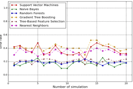
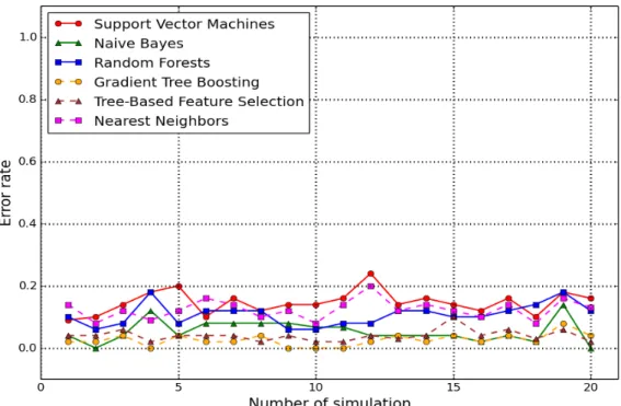
WSN strategies that can be considered are: the topologies, coverage, deployment strat-egy, scheduling mechanism, density, security, data aggregation, frequency, packet trans-fer distance, battery, memory, etc. These strategies have a strong impact on the effective-ness of the network with time, consequently on the quality of the data that will be captured, and finally on PHM. Although both PHM and WSN strategies have been studied, as far as we know, none of the existing research work has considered the WSN strategies for PHM. For instance, in real life application, the monitored area might not be fully covered for several reasons like nodes failure, energy depletion, unadapted initial deployment, scheduling mechanisms, etc. Obviously, this flaw may lead to inaccurate and incomplete data, and if we do not take such issue into consideration while building a PHM process over a WSN, the results provided by diagnostic or prognostic may not be reliable. There-fore, in this thesis we will study the WSN strategies and their relation with prognostic and health management. We will focus on the impact of these strategies on the accuracy of the data captured by a wireless sensor network, and its consequences on the health di-agnostic. To reach this goal, to evaluate both prognostic and health management with the WSN strategies, and to evaluate the importance of the random forest algorithm, we will use in WSN the random forest algorithm and five other diagnostic algorithms from litera-ture. Namely Support Vector Machines (SVM), Naive Bayes (NB), Gradient Tree Boosting (GTB), Tree-Based Feature Selection (TBFS), and Nearest Neighbors (NN) methods.
Hence, a dependable WSN should be used in the monitoring process. Coverage is one of the most important measurements of WSNs quality of service, and it is closely related to the energy consumption of sensors [125]. Thus, when designing WSNs, one of the most important challenges remains in the efficient use of these sensors, to increase the network’s lifetime while guaranteeing high coverage rate. The coverage rate and the con-sumption energy are the two most important factors in WSN, and these two factors are obviously proportional to each other. Indeed, the coverage rate increases when the num-ber of active sensors increases, but energy consumption increases accordingly. All of the research mentioned in the literature support the WSN by increasing the lifetime and maxi-mizing the coverage rate of the network, thus making it more efficient with time. However, numerous problems can be emphasized in these solutions, and are often application ori-ented. There is always a priority for these solutions in which they are either oriented to maximize the coverage or to maximize the lifetime of the network. All the attempts tried to compromise between these factors were not efficient.
Then, to solve this issue, we will propose in this thesis a reliable algorithm in graph theory for diagnostics and health management of the monitoring targets, by using the domi-nating sets proposed in [85, 12]. The proposed algorithm is completely distributed: no centralized or intermediate control is needed. This is a hybridization of three variants of domination in the sensors-targets graph, namely the simple, double, and total ones, in a single algorithm, which makes the originality of our study. To illustrate the efficiency of this approach and its impact on the accuracy of diagnostics, we will use the six machine learning algorithms mentioned before that have been used to diagnose the area state. These learning processes are evaluated in a WSN context with the proposed algorithm. By relying on this algorithm, the data diagnostics (PHM) will be accurate for the longest time possible.
1.1/
D
ISSERTATIONO
UTLINEThe remainder of this thesis is organized as follows :
Chapter 2 presents an overview to show the advantages and disadvantages of each of
wireless sensor networks and prognostic and health management. It also discusses the challenges of wireless sensor network monitoring in terms of industrial prognostics and health management. Finally, this chapter emphasizes what needs to be tackled in order to obtain good results.
Chapter 3 proposes the use of the random forest algorithm for diagnostic. The algorithm
is used for diagnosing the state of an industrial device when there are incomplete mon-itoring parameters via a WSN. This method is confirmed by computer simulations while varying the data collection process.
Chapter 4 this chapter studies and shows the impact of WSN strategies on
diagnostic-s/PHM, by relying on random forest algorithm and other algorithms in the literature. It also evaluates both prognostic and health management with the WSN strategies and the importance of the random forests algorithm suggested in Chapter 3.
Chapter 5 proposes effective and reliable distributed algorithm that relies on scheduling
mechanism to increase the network lifetime. And also to increase the coverage rate to the maximum (it’s able to compromise between these two factors) with the use of certain amount of active sensors in network.
Chapter 6 summarizes the work that was achieved and enumerates the contributions of
this thesis. It also discusses the perspectives.
1.2/
P
UBLICATIONS1.2.1/ PUBLISHED PAPERS
1. Impacts of wireless sensor networks strategies and topologies on prognostics and
health management. Ahmad Farhat, Christophe Guyeux, Abdallah Makhoul, Ali Jaber, Rami Tawil, and Abbas Hijazi. Journal of Intelligent Manufacturing (JIMS).
2. On the topology effects in wireless sensor networks based prognostics and health
management. In 19th IEEE International Conference on Computational Science and Engineering (CSE 2016), pages 1-9. IEEE, IEEE, aug 2016. Ahmad Farhat, Abdallah Makhoul, Christophe Guyeux, Rami Tawil, Ali Jaber, and Abbas Hijazi.
3. Random Forests for Industrial Device Functioning Diagnostics Using Wireless
Sen-sor Networks. IEEE AEROSPACE CONFERENCE, 2015. Big Sky, Montana, USA (2015, Pages 1-9). Wiem Elghazel, Jacques Bahi, Ahmad Farhat, Christophe Guyeux, Mourad Hakem, Kamal Medjaher, Noureddine Zerhouni.
1.2.2/ SUBMITTED PAPERS
4. Distributed Minimal Dominating Sensor-Targets for Diagnostics and Health
Man-agement. Ahmad Farhat, Christophe Guyeux, Mohammed Haddad, Mourad Hakem, and Abdallah Makhoul. Submitted to IEEE International Conference on Pervasive Computing and Communications.
5. A study on the Impact of Network Topology on Wireless Sensor Networks
Perfor-mance based on Prognostics and Health Management. Ahmad Farhat, Christophe Guyeux, Abdallah Makhoul, Ali Jaber, Rami Tawil, and Abbas Hijazi. Submitted to Journal of Ad Hoc & Sensor Wireless Networks (AHSWN).
6. On the coverage effects in wireless sensor networks based prognostic and health
management. Ahmad Farhat, Christophe Guyeux, Abdallah Makhoul, Ali Jaber and Rami Tawil. Submitted to International Journal of Sensor Networks (IJSNET).
S
CIENTIFIC BACKGROUND
I
n this chapter we will present an overview on wireless sensor networks and on prognos-tics and health management, to show the importance and characteristics of both, and their usefulness in real life. Furthermore, we will detail the links that can be established between these fields of research. And we will draw the challenges related to wireless sensor network based monitoring, which will lead to various solutions proposed in the contribution part of this manuscript.2.1/
A
N OVERVIEW ONW
IRELESSS
ENSORN
ETWORKSIn the last few years Wireless Sensor Networks (WSNs) have gained much attention in both public and research communities, caused by wealth of theoretical and practical chal-lenges [8], and because they are expected to bring the interaction between humans, en-vironment, and machines to a new paradigm. Even though it is an appealing topic which holds vision of an upcoming world, a huge gap still exists in the realizations of WSNs. This continuous research in WSNs has explored a variety of new applications enabled by larger scale networks of sensor nodes which are able to sense information from the environment, process the sensed data, and transmits it to the remote location [42, 94]. The wide growth of WSN is due to the improvement in low cost wireless communica-tion and micro-electro-mechanical systems [9]. These networks are wildly spreading due to their easy deployment and low cost. A while ago, transferring data from one unit to another requested expensive wiring. Currently, nodes can be placed almost anywhere, having no wiring contrasts, with any geographic or placement problems, and this is be-cause of the minimal batteries feeding the nodes. Sensors have the advantage of being used even discreetly due to their small dimensions. These advantages permitted the deployment of WSN in various fields, such as: medicine, military, agriculture, environ-mental, home automation, etc. Generally, a WSN is composed of few base stations (one in most cases) and a large number of sensor nodes. The main role of these devices is to monitor physical or environmental conditions, and to cooperate to deliver the sensed data to a base station called the sink. An example of wireless sensor networks is shown in Figure 2.1.
WSN are composed by very small sensors with very limited and nonrenewable energy. In order to preserve this energy, network throughput has to be low. An issue lies which is, as all wireless sensor networks, WSN are not very secure. A node failure (or attack) can occur due to both limitation of energy, and random deployment in hostile and inaccessible
Fig. 2.1: Wireless Sensor Networks monitoring.
areas [117]. Moreover, they do not dispose with a predefined infrastructure and this fact emphasizes the importance of the chosen routing protocol. A reliable communication should be ensured by an adequate protocol. This reliability means reducing data loss, fastening communication, minimizing energy consumption, and other standards.
WSN are event-based systems that rely on the collective effort of several sensor nodes [7]. This type of network tends to greatly increase the coverage rate for the area that should be monitored and also increase the accuracy of the information extracted from this area. The network extends the computational capability to reach the physical environments that are unreachable by the human beings. Generally, since sensor nodes function at a low frequency, they are not located far from each other. Because of that, there is a high possibility that many nodes sense the same data. This redundancy oc-curring will cause all the useful energy to be dissipated in vain if all of this redundant information was routed through the network.
In the next section, we will introduce a general overview of WSNs. This encompasses their advantages, and their drawbacks.
2.1.1/ SYSTEMS SOFTWARE FOR WSNS
A general-purpose operating system (OS) is an example of systems software. Due to the scarceness of resources and simplicity of applications, early WSNs did not include systems software. However, systems software is a requirement in complex applications because it facilitates the control of resources and increases the predictability of execution. Common interfaces provided by the software can hide the heterogeneity of platforms. Still, heavy computation and memory usage are the major disadvantages. The systems software for WSNs implement single node control and network-level distribution control. The low-level routines in a node are implemented by the single node control software, whereas application execution within several nodes is managed by the network-level dis-tribution control.
Fig. 2.2: Reference hardware platform architecture of a sensor node.
unit consists of CPU, storage devices, and an optional memory controller for access-ing the instruction memory of the main CPU. A sensaccess-ing unit consists of sensors and an analog-to-digital converter (ADC). The communication with other sensor nodes is enabled by a transceiver unit. A power generator that harvests energy from environment can be used to extend a power unit. Other peripheral devices, depending on the application re-quirements, are attached to the node, like peripheral actuators for moving the node and location finding systems [9]. The reference values in Figure 2.2 are the resources avail-able in MICA2 mote [1]. The power consumption of a node when active is in order of mW and in order of µW when the node is in sleep. The power unit is typically an AA battery or similar energy source.
OS or virtual machine (VM) accomplishes the single node control. In the reference plat-form, OS is executed on the main CPU and it uses the same instruction and data mem-ories as applications. OS implements services that include scheduling of tasks, Inter-Process Communication (IPC) between tasks, control of memory, and possible power control in terms of voltage scaling and component activation and inactivation. Interfaces to access and control peripherals are provided by OS. The interfaces are typically associ-ated with layered software components with more sophisticassoci-ated functionality, for example a network protocol stack.
Depending on the target application (mainly its goals and limits), a network setting is chosen, and the routing protocol will be developed accordingly. The protocol stack of sensor networks is composed of five different layers [9], which are shown in Figure 2.3.
1. Physical layer: it explains the ways of transmitting data packets after being
con-verted into raw data bits which are suitable for transmission over the communication medium. Basically, this layer is responsible for frequency selection, signal detection, modulation, carrier frequency generation, and data encryption.
2. Data link layer: it is charged of data stream multiplexing, data frame creation,
medium access, and error control to provide reliable transmission. It is also in charge of the creation of the network infrastructure, transferring data, and shar-ing the communication resources fairly and efficiently between sensor nodes, for
Fig. 2.3: Protocol stack for WSN.
achieving good network performance in terms of energy consumption, network throughput, and delivery latency. It is also responsible for error control of trans-mission data.
3. Network layer: it is responsible for routing the data from the source nodes until the
sink. It also allows inter-networking with external networks, where the sink node can be used as a gateway. It controls and orders the system, forwards data packets, and takes charge of routing between intermediate routers. Also, it ensures inter-networking with external networks.
4. Transport layer: its responsibility is the end-to-end data delivery between sensor
nodes and the sink. Traditional transport protocols cannot be applied directly to WSNs because of energy, computation, and storage constraints. Also, this layer provides other services like multiplexing, reliability, congestion avoidance, flow con-trol, etc.
5. Application layer: several protocols are included which perform various sensor
applications like time synchronization, query dissemination, node localization, net-work security, etc. It can be defined as the user interface. It shows messages in a human recognizable and understandable format.
WSN are broadly spread because of their low cost, easy deployment, and their capacity to extract localized features. Currently, they can be found in nearly all monitoring applica-tions. However, as far as we know, the literature of Prognostic and Health Management (PHM) does not report the use of this technology. Nevertheless, in some industrial appli-cations, the WSN monitoring can be obligatory.
2.1.2/ SENSOR NETWORK APPLICATIONS
Sensor networks may consist of many different types of sensors such as seismic, low sampling rate magnetic, thermal, visual, infrared, acoustic and radar, which are capable of monitoring a wide variety of ambient conditions that include the following [40]:
• temperature, • pressure, • humidity, • soil makeup, • vehicular movement, • noise levels, • lightning condition,
• the presence or absence of certain kinds of objects,
• current characteristics such as speed, direction, and size of an object.
Sensor nodes can be used for detecting events, event ID, sensing location, and local control of actuators. The concepts of micro sensing and wireless connection of these nodes hold many promises in new application areas. The applications are categorized into, environmental, military, home, health, and other commercial areas. Expanding this classification with more categories is possible such as space exploration, chemical pro-cessing and disaster relief.
2.1.2.1/ ENVIRONMENTAL APPLICATIONS
Some of the environmental applications of sensor networks include tracking movements of small animals, birds, and insects; monitoring environmental conditions affecting live-stock and harvest; precision agriculture; flood detection; pollution study; bio-complexity mapping of the environment; irrigation; chemical/biological detection; forest fire detec-tion; macro-instruments for large-scale Earth monitoring and planetary exploradetec-tion; me-teorological or geophysical research; biological, Earth, and environmental monitoring in marine, soil, and atmospheric contexts [5, 17, 22, 28, 27, 30, 59, 61, 120].
2.1.2.2/ MILITARY APPLICATIONS
Wireless sensor networks can be an essential part of military command, control, commu-nications, computing, intelligence, surveillance, reconnaissance and targeting (C4ISRT) systems. Sensor networks are considered a very promising sensing technique for military C4ISRT because of their rapid deployment, self-organization and fault tolerance charac-teristics. Sensor networks are based on the dense deployment of disposable and low-cost sensor nodes, so when some nodes are destructed by hostile actions, military operations aren’t affected as much as when a traditional sensor is destructed, thus making sensor
network concept a better approach for battlefields. Some of the military applications of sensor networks are battlefield; targeting; monitoring friendly forces, equipment and am-munition; nuclear, biological and chemical (NBC) attack detection and reconnaissance; reconnaissance of opposing forces and terrain; surveillance; and battle damage assess-ment.
2.1.2.3/ HOME APPLICATIONS
• Home automation: with the advancement in technology, smart sensors and
actu-ators can be placed in appliances like vacuum cleaners, microwave ovens, refriger-ators, and VCRs [89]. These sensor nodes can interact with each other inside the domestic devices and with the external network via internet or satellite. They allow the management of home devices locally and remotely more easily by end users.
• Smart environment: two different perspectives can be found for the design of
smart environment, i.e., centered and technology-centered [3]. For human-centered, a smart environment has to adapt to the needs of the end users in terms of input/output capabilities. For technology-centered, new hardware technologies, networking solutions, and middleware services have to be developed. A scenario of how sensor nodes can be used to create a smart environment is described in [54]. The sensor nodes can be embedded into furniture and appliances, and they can communicate with each other and the room server. Communication can also oc-cur between the room server and other room servers to learn about the services they offered e.g., printing, scanning, and faxing. These room servers and sensor nodes can be integrated with existing embedded devices to become self-organizing, self-regulated, and adaptive systems based on control theory models as described in [54]. The “Residential Laboratory” at Georgia Institute of Technology set another example of smart environment [38]. Computing and sensing in this environment should be persistent, reliable, and transparent.
2.1.2.4/ HEALTH APPLICATIONS
Interfaces are being provided for sensor networks by some of the health applications for the disabled, integrated patient monitoring, diagnostics, drug administration in hospitals, telemonitoring of human physiological data, tracking monitoring doctors and patients in-side a hospital, and monitoring the movements and internal processes of insects or other small animals [22, 61, 84, 93, 120].
2.1.2.5/ OTHER COMMERCIAL APPLICATIONS
Some of the commercial applications are tracking and detection of vehicles; monitoring material fatigue; environmental control in office buildings; interactive museums; building virtual keyboards; machine diagnosis; automation and factory process control; inven-tory managing; smart structures with sensor nodes embedded inside; interactive toys; car thefts monitoring and detecting; product quality monitoring; constructing smart office spaces; factory instrumentation; transportation; local control of actuators; robot control and guidance in automatic manufacturing environments; monitoring disaster area; and
instrumentation of semiconductor processing chambers, rotating machinery, wind tun-nels, and anechoic chambers [40, 39, 92, 91, 98, 5, 30].
2.1.3/ SHORTCOMINGS OF A WSN
The purpose of designing WSNs is for efficient event detection. Consisting of a large number of sensor nodes deployed in a surveillance area, they are able to detect the occurrence of new events Efficiency is a necessity in such activities, which is hard to achieve with the constraints of WSNs. These limitations are detailed in the following.
2.1.3.1/ RESOURCES
What mostly limits the WSN capabilities is the available energy. The sensors are small sized devices, with tiny batteries as an energy supply. Moreover, the nodes are often deployed in hostile environments (mountains, enemy territory, etc.) where they cannot be recharged [26].
Another important impact on the available energy for normal network tasks is the added security. Extra power is necessary for processing security functions (encryp-tion, decryp(encryp-tion, signing data, verifications), transmitting security related data (vectors for encryption/decryption), and securing storage (cryptographic key), which is critical for WSNs [26, 117].
In addition to this, there is a very limited memory space deployed for a sensor node. The communication protocol and the security code share the storage space. The size of the latter has then to be limited to a minimum [117].
There is also a limited buffering space in sensor nodes. With the increase in traffic flow towards the sink node, this will lead to packet loss. As a matter of fact, with new packets coming in, a sensor node cannot hold data packet for a long period. All the nodes will attempt to get rid of the old messages, in the case of a high traffic flow, to make space for the new ones by forwarding them to the next level. Therefore, as all sensor nodes tend to forward the captured data to the sink, the area around the sink tends to be quickly congested.
2.1.3.2/ COMMUNICATION
Wireless communication is known to be unreliable and it adds to the network’s vulnera-bilities. The absence of physical connections can result in:
• Channel errors: occurring at the recipient, wrong signals may arrive because of
the noise in communication channels.
• Missing links: invalid or missing links between the sensors and consequent packet
drop is caused by route updates, interference in the radio channels, energy exhaus-tion, etc.
• Communication latency: greater latency is achieved by both multi-hop routing and
is the latency. Extra delays are taken into consideration when re-transmission is required for transmission errors. One of the major drawbacks of latency is that it makes synchronization among nodes hard to achieve.
• Network congestion: Dense packet exchange in the network reflects heavy traffic,
and a concurrent access may present itself at certain regions. The Quality of service (QOS) of a node carrying so much data degrades as this leads to packet collision, packet loss, transmission delays, etc.
Most WSNs are deployed in harsh environment conditions and/or are exposed to ad-versary attacks. This can cause permanent (even irreversible) damage to the hardware because of the likelihood of physical attacks. The sensor nodes can be left unattended for a long period of time since the network is remotely managed. Therefore, detecting physical tampering or performing regular maintenance would be difficult, and thus, the network would remain unable to fulfill the intended tasks [117].
Routing solutions in WSNs avoid central management point as it results in a single point of failure. This complicates the synchronization among nodes, and lowers packet delivery rate. Synchronization among nodes should be ensured which necessitates access to extra memory space to improve the communication protocol, consuming more resources.
2.2/
P
ROGNOSTICS ANDH
EALTHM
ANAGEMENTMaintenance is an important activity in industrial field. It is carried out to either restore a machine/component, or prevent its break down. Its aim is to increase system availability, readiness, thus enhancing safety. Throughout time, vairous strategies have evolved and were developed to bring maintenance to its current state: condition-based and predictive maintenance. What caused this evolution was the increasing demand of reliability in industry. Prognostics and Health Management (PHM) is a tool to predict the Remaining Useful Life (RUL) of engineering assets and is the key process of condition-based and predictive maintenance. At the present days, industrial machines are needed to avoid shutdowns while offering safety and reliability [88]. A great deal of attention was given to research in PHM field. Prognostic models are developed in an attempt to predict the RUL of machinery (or monitored area) before failure occurs. It is possible that the maintenance activity will be performed either too soon or too late, if the prediction model and the provided measurements are not accurate.
In Condition-Based Maintenance (CBM) and Predictive Maintenance (PM), the use of monitoring devices is for surveying the physical condition of the equipment. A mainte-nance activity should be performed when a certain level is reached (threshold) to ensure the continuity of the machine/system’s normal functioning. CBM and PM require extra investments related to the monitoring equipment, in comparison to corrective and pre-ventive maintenance. Nevertheless, it increases the system’s availability and optimizes the service life, all while reducing downtime and avoiding unnecessary maintenance. Be-cause of the advantages of Condition based maintenance in comparison to other strate-gies, its use is privileged. A comparison is summarized in Table 2.1.
The core activity of CBM and PM is Prognostics and Health Management (PHM). The steps of PHM are: data acquisition, data processing, health assessment, diagnostics,
Strategy Advantages Drawbacks
Corrective maintenance -Low cost
-Service life is fully exploited
-Sudden failures -High repair costs
-Dangerous failure outcomes
Preventive Maintenance
-Improved availability -Decreased downtime -Costs saving
-Unplanned downtime -Unneeded repair costs -Interrupted service life
Condition-based
and predictive maintenance
-Increased availability -Reduced downtime -Reduced costs
-Optimal system service
-Investment in monitoring equipment
Table 2.1: Comparison of maintenance strategies.
prognostics, and decision making support [60]. This is done following the steps described in Figure 1.3, and explained in details in the following sections.
2.2.1/ DATA ACQUISITION
Prognostics and Health Management (PHM) requires information about the targeted physical assets. The sensors which are placed on/around the critical components acquire the data. Later on, the developed algorithm will be fed stored data as inputs for health assessment, diagnostics, and/or prognostics. Here we can observe the significance of the quality of the data as all of the next steps rely on these measurements. The gathered information can contain either event-data or Condition Monitoring (CM) data. Event-data reveal what happened, what were the causes, and what was done (repair, breakdown, installation, etc.). CM data, on the other hand, contains measurements that are related to the condition of the machine (pressure measurements, environment data, etc.). These two types of information are of equal importance for health assessment, diagnostics, and prognostics. In Figure 2.4, a summary of data acquisition steps is given.
2.2.2/ DATA PROCESSING
Performing data cleaning is very important once the information is available and before building the degradation model, in order to enhance the results of health assessment, di-agnostics, and prognostics. The importance of processing the data consists in providing signals that are robust against the variations that might affect the raw data since com-municating channel might induce errors [95]. Its aim is to isolate all the possible errors and avoid the so-called ”garbage in, garbage out” problem. Authors of [13] defined data processing as the collection and manipulation of items of data to produce meaningful raw data.
In practice, raw sensor signals can be complex, and data describing the degradation is not easy to read. Reported data can have a value type, a waveform type, or a multidi-mensional type. The last two types are very hard to exploit since they can contain noise. Data processing is considered an important step as it converts raw data into useful infor-mation. Prognostic literature have reported many processing techniques [83, 110], like wavelet decomposition, data smoothing, data denoising, etc.
Fig. 2.5: Data processing system.
Data processing can be divided into two main tasks: (1) pre-processing of sensor raw signals and (2) data analysis for more information extraction. The aim of this step is to improve the signals that are being received from the monitoring device, to provide a better understanding of the process that generated the data, to enhance the degradation model, and to render the computation more effective by reducing the measurement size. The steps of a data processing system are given in Figure 2.5.
2.2.3/ HEALTH ASSESSMENT
Health assessment consists of determining the state of health of the system at a given time. For that, sensory data are reported periodically to monitor critical components. These data correspond to measurements of relevant parameters (moisture, pressure,
temperature, etc.), and are useful in assessing the condition of the machine. Thresholds related to the monitored parameters are fixed. The system is considered to be in the corresponding state once a threshold is reached (See Figure 2.6).
Fig. 2.6: Health assessment process.
Health assessment task can be narrowed down to a classification problem, and there exist several ways to perform this task. For instance, human expertise can be the basis for identifying the class to which belongs a functioning profile. This needs a solid knowledge based on both experience and history of observations of the application domain. This knowledge will help in deriving rules relating an observation to its meaning and also can be explored to develop mathematical models describing the physics of the system under consideration. On-line measurements can be run through the developed model to identify the health state. This problem can also be solved by machine learning techniques. Off-line observations will be used to train a model which will then be used on-Off-line to determine the class of new observations.
2.2.4/ DIAGNOSTICS
After the fault has taken place, diagnostics is performed. It identifies the type of fault, its size, location, and cause. The aim of diagnostics is then to relate the cause to the effect. It is an understanding of the relationship between what we observe and what happened before [99]. Figure 2.7 illustrates the successive steps of diagnostic process.
Fig. 2.7: Diagnostics different steps.
1. Fault detection is the process of reporting an anomaly in the system’s behavior. 2. Fault isolation is charged of determining and locating the cause (or source) of the
problem. It identifies exactly which component is responsible of the failure.
3. Fault identification aims at determining the current failure mode and how fast it can
2.2.5/ PROGNOSTICS
The aim of diagnostics is to identify and quantify an actual failure, while the goal of prog-nostics is to anticipate failures. There exist several definitions concerning progprog-nostics in the literature. We summarized some of them in Table 2.2.
Definition Authors Reference
Predicts how much time is left before a failure (or more) occurs, given the current machine condition and past operation profile.
K.S. Jardine et al. [60] Indicates whether the structure, system, or component
of interest can perform its function throughout its lifetime with reasonable assurance and, in case it cannot, to estimate the remaining useful life.
Zio and Di Maio [126]
Estimation of the time before failure, or the remaining useful life, and the associated confidence value.
Tobon-Mejia et al. [110, 111] Estimation of time to failure and risk for one
or more existing and future failure modes. ISO 13381-1 [80] Table 2.2: Some definitions of prognostics reported in the literature.
For estimating the RUL, prognostics consider past events, the machine’s current state, and operating conditions. By inspecting the evolution of continuous measurements of parameters that need to be monitored in, this estimation is done in order to assess the machine’s state. These parameters can be temperature, humidity, vibration, pressure, and so on. A monitored parameter has a fixed threshold. Once this threshold is reached, an alarm goes off indicating the detection of a symptom of system deterioration. The RUL is then computed with an associated confidence limit. The latter information illustrates to what point the predictions are trustworthy. There are two causes for the uncertainties of the RUL predictions: it is either threshold value of monitored parameter, or the RUL prediction itself. Figure 2.8 shows uncertainties concerning prediction of RUL.
Collection of documented data covering the machinery and components under consider-ation is required for an efficient prognostic activity. All monitored parameters and descrip-tors need to be available with historical records of operations and events. For improving the prognostics results, failure identification and initial diagnostics are also obligatory [80].
2.2.6/ DECISION SUPPORT SYSTEM
The next step after performing prognostics and estimating RUL, is deciding the actions that need to be taken (repair, replacement, maintenance, oil changing, etc.). Decision making is a cognitive process. It consists of selecting an action among different possible scenarios, to produce a final choice. Figure 2.9 describes the general process.
Fig. 2.9: Decision support system.
First of all, the objectives need to be established. An objective can be keeping component from failure until next inspection, reducing overall costs, or any other purpose a plant can be aimed for. Then, all the objectives are classified according to their priority and impor-tance. In order to answer the established objectives, alternative actions are developed, and the actions satisfying most of the objectives are selected. A decision needs to be made to select the appropriate action. This can be done by implementing a tool among different possibilities.
• Domain experts: very often, plants trust the advice that the engineers and experts
in the domain provide them with. They are able to come up with good solutions and reveal the limitations related to a strategy.
• Eliminations: further solution is eliminating non-realistic solutions one by one, or
comparing them in a pairwise manner. Lastly, the remaining option is selected.
• Analytic networks: these networks provide a hierarchy of the selected action with
goals, alternatives, and consequences.
• Simulations: for visualizing the system’s behavior under different conditions, many
graphical tools exist. Simulations are a well-known tool for decision making support since they offer clarity and possibility to alter criteria while simulating.