HAL Id: hal-01824023
https://hal.archives-ouvertes.fr/hal-01824023
Submitted on 28 Jun 2018
HAL is a multi-disciplinary open access
archive for the deposit and dissemination of
sci-entific research documents, whether they are
pub-lished or not. The documents may come from
teaching and research institutions in France or
abroad, or from public or private research centers.
L’archive ouverte pluridisciplinaire HAL, est
destinée au dépôt et à la diffusion de documents
scientifiques de niveau recherche, publiés ou non,
émanant des établissements d’enseignement et de
recherche français ou étrangers, des laboratoires
publics ou privés.
Tom Peterka, Hadrien Croubois, Nan Li, Esteban Rangel, Franck Cappello
To cite this version:
Tom Peterka, Hadrien Croubois, Nan Li, Esteban Rangel, Franck Cappello. Self-Adaptive Density
Estimation of Particle Data. SIAM Journal on Scientific Computing, Society for Industrial and Applied
Mathematics, 2016, 38 (5), pp.S646 - S666. �10.1137/15M1016308�. �hal-01824023�
TOM PETERKA∗, HADRIEN CROUBOIS†, NAN LI‡, STEVE RANGEL§,ANDFRANCK CAPPELLO¶
Abstract. We present a study of density estimation, the conversion of discrete particle positions to a continuous field of particle density defined over a 3D Cartesian grid. The study features a methodology for evaluating the ac-curacy and performance of various density estimation methods, results of that evaluation for four density estimators, and a large-scale parallel algorithm for a self-adaptive method that computes a Voronoi tessellation as an intermediate step. We demonstrate the performance and scalability of our parallel algorithm on a supercomputer when estimating the density of 100 million particles over 500 billion grid points.
Key words. Density estimation, cloud in cell, smoothed particle hydrodynamics, Voronoi tessellation, nearest grid point, triangular shaped clouds
AMS subject classifications. 51-04, 68-04, 70-04, 85-04.
1. Introduction. In the context of scientific data analysis, density estimation is a trans-formation from discrete particle data to a continuous density function defined over a 3D field. This field can be interpolated, differentiated, and integrated: operations not possible in the particles’ original discrete form. Moreover, the density field is discretized by a regular grid, which offers several advantages. (1) It is compact, in that x, y, z coordinates of the grid points are defined implicitly and need not be stored. (2) Applications using a regular grid are readily parallelizable because subdomain decomposition and processor assignment are also regular and implicit. (3) A regular grid is the most common data model for scientific data analysis and visualization algorithms. For example, most of the volume rendering literature in the past
25 years targets regular grids [9,24,37]; far less exists for adaptively refined grids [23] and
unstructured meshes [30].
Density estimation is a fundamental step needed whenever a discrete particle dataset is sampled over a continuous field. Our research is motivated by cosmology and astrophysics, but many other applications exist, for example estimating population density in geospatial applications or electron charge density in computational chemistry. Density estimation is also a key visualization step when an algorithm calls for a regular scalar field but particles are provided instead. For example, atom positions from molecular dynamics simulations may be converted to a grid before rendering an isosurface of atomic density.
One of the earliest and arguably most popular density estimators, cloud in cell (CIC), was introduced 45 years ago [7]. Since then, smoothed particle hydrodynamics (SPH) and tessel-lation (TESS) methods have emerged. Combinations and variations also exist: for example, characteristics such as the window shape of CIC and the adaptivity of SPH can be combined. Nevertheless, two questions remain unanswered: Which density estimators are appropriate for a given problem domain and computational budget, and how can the estimator of choice be scaled to today’s problem sizes? In this paper, we examine the first question by designing an evaluation methodology and showing how several estimators can be compared using it. Then, we show how a parallel algorithm can be constructed for one of those estimators.
We begin by explaining the common ideas in estimation methods such as window shape and weighting function; and we briefly explain the operation of four estimation methods, noting their strengths and weaknesses. After the background and related work, we present
∗Argonne National Laboratory[email protected] †ENS de Lyon
‡University of Chicago §Northwestern University ¶Argonne National Laboratory
Higher-order First-order
Zero-order
Cube Sphere Polyhedron
Window Shapes
Weighting FunctionsX
FIG. 1. Common window shapes and weighting functions in density estimation.
a methodology for designing synthetic datasets that mimic characteristics of actual data in a given application area. Our choice of design parameters is motivated by an application of density estimation in gravitational lensing to model the refraction of light rays caused by galaxies. The input data for lensing calculations comes from computational cosmology simulations. Using the datasets and test methodology we developed, we compare four density estimators with each other and with known analytical functions that underlie our particle data. We also derive the asymptotic time complexity of each of the four methods.
For our particular target of gravitational lensing, the TESS method turns out to be the best density estimator because it is relatively stable under small perturbations in particle sampling and therefore best captures the underlying density function. Because TESS needs no external parameters regarding window size or shape, it is entirely self-adaptive: the window over which a particle is deposited onto grid points adapts automatically to the size and shape of the Voronoi cell containing the particle. The paper concludes by describing a parallel algorithm for TESS that scales to high-performance computing (HPC) architectures; timing and scalability performance results are included.
Our work demonstrates that the choice of density estimator depends on characteristics of the target problem such as dynamic range, discontinuities, overall data size, and computa-tional budget. Despite the importance of selecting an appropriate density estimator to capture the underlying density function accurately and efficiently, after four decades CIC still remains the de facto technique used in simulations and visualization tools. In fact, the only density estimator available in VTK [42], ParaView [1], and VisIt [10] is a serial CIC filter. Our study shows that CIC, while inexpensive to compute, is inaccurate for datasets such as ours with high dynamic range.
The key contributions of our work are threefold: (1) we describe a methodology for designing synthetic data and comparing estimators quantitatively and qualitatively; (2) we present the results of that comparison for synthetic data representative of N-body cosmology codes; and (3) we present a large-scale parallel algorithm for estimating the density field of 3D particle data using a 3D Voronoi tessellation to automatically adapt to the particle distribution.
2. Background and Related Work. In this paper, we refer to the input dataset of 3D points as particles and to the locations on the regular grid where the output density values are computed as grid points. It does not matter whether density values are vertex-centered (at the grid lines) or cell-centered (at the grid spaces); by convention, our terminology is
vertex-CIC
SPH
ACIC
TESS
FIG. 2. Density estimation methods studied in this paper. In cloud in cell (CIC), particles are distributed to a fixed number of grid points, usually 8 in 3D, using first-order weighting. Smoothed particle hydrodynamics (SPH) use fixed-shape spherical windows whose size also adapts to contain the same number of particles; weighting is higher-order, usually Gaussian. In adaptive CIC (ACIC), the number of grid points adapts to encompass a fixed number of particles, and the weighting may be zero-, first-, or higher-order. In tessellation (TESS) methods, particles are distributed in windows of variable size and shape using zero-order weighting.
centered. We define density estimation as the process of distributing some property of the particles (we use particle mass in this paper, but the density of any property can be distributed) within an estimation window weighted according to a weighting function. Irrespective of the window and weighting, any estimation method must obey the conservation of physical properties; in our case, total particle mass is conserved.
2.1. Estimation Windows and Weighting Functions. We categorize different density estimators according to their estimation windows and weighting functions. The estimation window associated with a given particle is the region of grid points over which the particle’s mass is distributed. The weighting function determines the fraction of the particle mass
de-posited on each grid point in the window. Figure1 shows three window shapes and three
weighting functions. The window shape (cube, sphere, or polyhedron) may be either fixed or adaptive size. In this paper, the weighting function (zero-, first-, or higher-order) is a uniform distribution, linear interpolation, or Gaussian distribution, respectively. Window shapes and weighting functions can be combined in various ways; in this paper we examine four density
estimation methods with various window shapes and weighting functions. Listed in Table1,
they are cloud in cell (CIC), smoothed particle hydrodynamics (SPH), adaptive cloud in cell (ACIC), and tessellation (TESS).
2.2. Density Estimators. Figure2shows four classes of density estimators studied in
this paper; each class is identified by its window size and shape and weighting function as explained above. In addition to the four methods we studied, two others are mentioned at the end of this section, NGP and TSC.
2.2.1. Cloud in Cell Methods. CIC [7] is a first-order method that linearly interpolates the particle’s mass to neighboring grid points. CIC has a fixed size and shape window that encompasses eight grid points surrounding the particle. The weighting function distributes the mass of one particle to the eight adjacent grid points according to the distance from the particle to the grid points. Specifically, in 3D the mass of point P is distributed among the
surrounding grid points G0through G7. If the volume of the grid cell with corners G0, G7is
v(G0, G7) = 1.0, then the mass assigned to grid point Gi is m(Gi) = 1.0 − v(Gi, P). CIC is
used in many simulations; astrophysics [21] and plasma fusion [32] are two examples. CIC is easy to compute, but undersampling in low-density regions with insufficient numbers of particles in grid cells can produce noisy results. Despite its shortcomings, CIC remains the most popular density estimator for visualization and visual analytics. Pang and Albrecht [33],
TABLE1
Density Estimator Characteristics
Method Window Shape Window Size Weighting
CIC Fixed: cube Fixed: 8 grid points First-order
SPH Fixed: sphere Adaptive: min. # particles Higher-order
ACIC Fixed: cube Adaptive: min. # particles Higher-order
TESS Adaptive: polyhedron Adaptive: Voronoi cell Zero-order
for example, sample air traffic density onto a regular grid with CIC prior to volume rendering. 2.2.2. Smoothed Particle Hydrodynamics Methods. In order to overcome the limita-tions of CIC, the size of the window can adapt to cover some prescribed number of particles. SPH [29] has a spherical window with variable size; the window radius r is large enough to encompass T particles, where T is a parameter provided by the user. The window is centered on the input particle. The weighting function W (r) also must be specified; often a Gaussian is used. The main advantages of SPH are its adaptivity in window size and its ability to simultaneously act as a smoothing filter through its weighting function. Its disadvantage is the reliance on and sensitivity to the parameter T , the desired number of particles in a win-dow. SPH is widely used in astrophysics fluid dynamical computations [16] to estimate mass distribution for cosmic structure formation [6] and in other areas of science and engineering. 2.2.3. Adaptive Cloud in Cell Methods. Characteristics of CIC and SPH can also be combined. One such combination that we call ACIC (adaptive CIC) features a cube-shaped window as in CIC whose size adapts to cover a given number of particles as in SPH. Birdsall and Fuss [8] first mentioned variable-size particle clouds. Many adaptive mesh refinement (AMR) simulations, for example Nyx [2], deposit density on a grid using ACIC windows, where the window is prescribed by the AMR grid level of the solver. In statistics, adaptive kernel density estimators (AKDE) [39,43,45] for computing a 1D probability density function (PDF) are a closely related topic. In both AKDE and ACIC, the kernel width adapts to a given number of input points, but the ACIC kernel is a 3D cube whose density does not integrate to 1, whereas AKDE has a 1D kernel over which a single or multivariate PDF is estimated. Lukasik [26] parallelized the (fixed-size) KDE using MPI, and Michailidis et al. [28] accelerated KDE for GPUs, but we have not found any parallel algorithms for (variable-size) AKDE in the literature. Our implementation of ACIC uses a cube-shaped window aligned with and centered on the grid cells, and we adapt the window symmetrically in three dimensions until it covers the desired number of particles. As in SPH, the advantage of ACIC is its adaptive size, and its drawback is selecting T , the number of input particles in the window.
2.2.4. Tessellation Methods. Both the window size and shape vary in TESS, which is self-adaptive and driven entirely by a Voronoi tessellation. The advantage of TESS is its self-adaptivity without reliance on any parameters. The estimation window is the Voronoi cell, and the weighting function distributes particle mass over the grid points in the window. The most expensive parts of the algorithm are computing the tessellation and finding the intersection of grid points with Voronoi cells. Our TESS method resembles the DTFE of
Schaap and Van de Weygaert [40,41]. The main three differences between our work and
theirs are: the DTFE used a Delaunay tessellation with first-order interpolation, whereas we use a Voronoi tessellation with zero-order weighting instead; they compared resulting density images visually, whereas a main focus of our work is developing a systematic method for designing test datasets and quantifying the differences with several metrics; and we develop
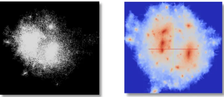
FIG. 3. Density estimation of one cosmological halo for gravitational lensing. Left: original raw particle data. Right: 2D density field.
an efficient parallel algorithm for the density estimation and evaluate its scalability.
2.2.5. Other Methods. For completeness, we mention two other methods often found in particle simulations [18]. The nearest grid point (NGP) method deposits the entire mass of the particle to the nearest grid point. It is a zero-order estimation method with a window size of one grid space, centered on each grid point. Not every grid point is necessarily covered by a window, making the density field discontinuous (noisy) in low-density regions where grid cells are devoid of particles. One may consider NGP to be a degenerate version of CIC, where the window covers only one grid point instead of eight. On the other hand, the triangular-shaped cloud (TSC) method may be viewed as an expanded CIC, where the window covers a fixed size of 27 (3 × 3 × 3) grid points. Each particle is deposited onto its nearest 27 grid points using first-order weighting.
3. Synthetic Data Design. The regular grid estimation of particle density has many uses in science and engineering; we begin by describing one such application, gravitational lensing. Next, we describe a parameterized method for constructing synthetic input particle datasets with known underlying analytical density functions. The parameters of the datasets are derived from the characteristics (density range, substructure, anisotropy) of the target application. In this way, we can represent actual data while having a ground truth for com-parison. We then describe ways to carry out this comcom-parison.
3.1. Motivation: Gravitational Lensing. The deflection of light when passing through
a gravitational potential is called gravitational lensing [5,20]. Optical distortion caused by
lensing is observed at all scales in the universe, making gravitational lensing a powerful tool for investigating dark matter and dark energy [27]. Gravitational lensing is simulated by computing the gravitational potential from the continuous density field of dark matter parti-cles modeled by an N-body cosmological simulation [38]. To compute an accurate lensing simulation, one must have a density field that is low in noise, that reflects the underlying continuous density function, and that scales to the size of the simulation.
Figure3shows one cluster of dark matter particles whose density is estimated onto a 2D
grid. For lensing calculations, the lens is modeled as a 2D density field located far away from the observer. Because the particles are in 3D, however, the density is estimated in 3D first before projecting to 2D. The input particles are produced by computational cosmology codes such as HACC (Hardware/Hybrid Accelerated Cosmology Code), a Gordon Bell finalist
N-body code that exceeded 10 petaflops [17]. In the left image of Figure3, we extracted one
cluster consisting of approximately 100,000 particles from the simulation output. The right image shows the estimated density field.
TABLE2
2D Density Images of NFW and CNFW
NFW CNFW NFW CNFW
CIC Density SPH Density
100 101 102 103 104 105 106 107 100 101 102 103 104 105 106 107 100 101 102 103 104 105 106 107 100 101 102 103 104 105 106 107
Ratio Analytical / CIC Ratio Analytical / SPH
10-2 10-1 100 101 102 10-2 10-1 100 101 102 10-2 10-1 100 101 102 10-2 10-1 100 101 102
ACIC Density TESS Density
100 101 102 103 104 105 106 107 100 101 102 103 104 105 106 107 100 101 102 103 104 105 106 107 100 101 102 103 104 105 106 107
Ratio Analytical / ACIC Ratio Analytical / TESS
10-2 10-1 100 101 102 10-2 10-1 100 101 102 10-2 10-1 100 101 102 10-2 10-1 100 101 102 Analytical Density 100 101 102 103 104 105 106 107 100 101 102 103 104 105 106 107
3.2. Analytical Functions. One may define analytical synthetic density functions to
produce desired data characteristics. For example, molecular dynamics [22,44] and
cosmol-ogy simulations [2,38], while both particle methods, have widely different behavior. We
begin with a simple symmetrical density profile whose parameters are chosen to mimic the density profile of a given problem. Next, we construct more complex analytical functions that superimpose several instances of the original function. In so doing, we apply different parameters to each component and produce more complex features in the synthetic data, all
the while maintaining a known analytical solution.
Our first analytical function is a spherical density profile derived from an NFW (Navarro-Frenk-White) function [31]:
ρ (r) = k
r(r + 1)2,
where ρ is the density; r is the radius, and k is a constant. The NFW function is an ideal testbed because it can model a high density range (ρ = ∞ at r = 0, and ρ = 0 at r = ∞). For our tests, we truncate the domain of r ∈ [−1.5, 1.5]; and we cap the range to a maximum ρ =
106, which approximates the density range of dark matter tracer particles in computational
cosmology.
In addition to high dynamic range, dark matter forms clusters of large-scale structures and substructures that are asymmetrical. To capture this behavior in our synthetic data, we compose several NFW models in a complex NFW model that we call CNFW. In our tests, the CNFW has eleven NFW components scaled with different values of k. Furthermore, we asymmetrically truncate the domain to create ellipsoidal structures. We also translate each component before composing them. Therefore, the CNFW allows us to test a dataset that is anisotropic, contains substructure, and more closely resembles the actual data in N-body simulations. Because the model is composed of analytical functions, however, we still know the ground truth density at any grid point, and we can compare the estimated and known density.
3.3. Input Particles. Monte Carlo sampling is used to produce discrete particle datasets from the analytical function. A random number is generated from a uniform distribution in [0, 1); the inverse of the cumulative distribution function of the NFW determines r, which is then converted to (x, y, z) coordinates of a particle by choosing the spherical angle coordinates from a uniform distribution. A single instance of a Monte Carlo particle set may be used to compare estimators with each other and with the specific instance of the input data; perform-ing the Monte Carlo sample multiple times (producperform-ing multiple particle datasets) can be used to better understand how well a density estimator captures the true underlying density that is represented by the particles.
3.4. Testing Methods. Each density estimator is then applied to the input datasets, pro-ducing a regular grid density field. All our tests are projected from a 3D density volume to a
2D density image, as explained in Section5.1, to simplify visualizing and comparing results.
In addition to visual inspection of the density images, images of the ratio of the analytical density divided by the estimated density are evaluated. Furthermore, cross sections through these images are taken to produce line plots. The power spectra of the density images are also analyzed to explain the estimation behavior in terms of spatial frequency.
4. Evaluation Results. Next, we demonstrate how to apply our design methodology in practice. Having constructed the NFW and CNFW analytical functions based on a particular science domain, we compare four density estimators as described above. Then we can decide
which estimator is best suited for our particular science problem. In Section4.1, we evaluate
the accuracy of four density estimators. The results for a single Monte Carlo particle dataset
appear in Tables2and3; Figure4shows results for an ensemble of 20 Monte Carlo datasets.
Section4.2compares the estimators in terms of their asymptotic computational complexity.
4.1. Accuracy. Table2shows the 2D density images for the four density estimators and
the NFW and CNFW analytical functions. Each of the four estimations includes the density image with the image of the ratio between the analytical and estimated density below. A
TABLE3
Cross Section of NFW and CNFW Density
NFW CNFW NFW CNFW
CIC Density SPH Density
1.5 1.0 0.5 0.0 0.5 1.0 1.5 X 101 102 103 104 105 106 2D Density
Analy. and CIC Estim. Density Analy. Estim. 1.5 1.0 0.5 0.0 0.5 1.0 1.5 X 101 102 103 104 105 106 2D Density
Analy. and CIC Estim. Density Analy. Estim. 1.5 1.0 0.5 0.0 0.5 1.0 1.5 X 101 102 103 104 105 106 2D Density
Analy. and SPH Estim. Density Analy. Estim. 1.5 1.0 0.5 0.0 0.5 1.0 1.5 X 101 102 103 104 105 106 2D Density
Analy. and SPH Estim. Density Analy. Estim.
Ratio Analytical / CIC Ratio Analytical / SPH
1.5 1.0 0.5 0.0 0.5 1.0 1.5 X
10-1
100
101
Analy. / Estim. Density
Analy. / CIC Estim. Density Analy. / Estim. 1.5 1.0 0.5 0.0 0.5 1.0 1.5 X 10⁻¹ 100 101
Analy. / Estim. Density
Analy. / CIC Estim. Density Analy. / Estim. 1.5 1.0 0.5 0.0 0.5 1.0 1.5 X 10⁻¹ 100 101
Analy. / Estim. Density
Analy. / SPH Estim. Density Analy. / Estim. 1.5 1.0 0.5 0.0 0.5 1.0 1.5 X 10⁻¹ 100 101
Analy. / Estim. Density
Analy. / SPH Estim. Density Analy. / Estim.
ACIC Density TESS Density
1.5 1.0 0.5 0.0 0.5 1.0 1.5 X 101 102 103 104 105 106 2D Density
Analy. and ACIC Estim. Density Analy. Estim. 1.5 1.0 0.5 0.0 0.5 1.0 1.5 X 101 102 103 104 105 106 2D Density
Analy. and ACIC Estim. Density Analy. Estim. 1.5 1.0 0.5 0.0 0.5 1.0 1.5 X 101 102 103 104 105 106 2D Density
Analy. and TESS Estim. Density Analy. Estim. 1.5 1.0 0.5 0.0 0.5 1.0 1.5 X 101 102 103 104 105 106 2D Density
Analy. and TESS Estim. Density Analy. Estim.
Ratio Analytical / ACIC Ratio Analytical / TESS
1.5 1.0 0.5 0.0 0.5 1.0 1.5 X
10-1
100
101
Analy. / Estim. Density
Analy. / ACIC Estim. Density Analy. / Estim. 1.5 1.0 0.5 0.0 0.5 1.0 1.5 X 10⁻¹ 100 101
Analy. / Estim. Density
Analy. / ACIC Estim. Density Analy. / Estim. 1.5 1.0 0.5 0.0 0.5 1.0 1.5 X 10⁻¹ 100 101
Analy. / Estim. Density
Analy. / TESS Estim. Density Analy. / Estim. 1.5 1.0 0.5 0.0 0.5 1.0 1.5 X 10⁻¹ 100 101
Analy. / Estim. Density
Analy. / TESS Estim. Density Analy. / Estim.
ratio of 1.0 (no error) corresponds to the color of the background in the corners of the image. Hence, one can easily see the error in the foreground by comparing its color with that of the background. CIC suffers from noise caused by undersampling over much of the image except the high-density center region. Low-density regions in the input data combined with a high-resolution grid can generate grid cells with zero particles; this situation is the primary drawback of CIC.
The other estimators do better except for the area near the boundary of the sphere or ellipsoid. This edge effect is caused by the an incomplete estimation window at the bound-ary. For example, the tessellation has incomplete Voronoi cells there; similarly, ACIC and SPH cannot compute windows with the desired number of particles at the edges. Such edge effects are inherent in these methods, and density values near the edge of a boundary must be discarded.
For a more quantitative comparison, Table3is a cross section through the y = 0 plane
of the data in Table2. Included are plots showing the cross section of estimated density
between analytical and estimated density. SPH, ACIC, and TESS all do better than CIC, but there are subtle differences visible upon zooming in on the CNFW slices of SPH, ACIC, and
TESS in Table3. SPH is the smoothest, but it misses sharp discontinuities; in particular, SPH
underestimates the maximum density at the two peaks of the CNFW. ACIC has more oscil-lations about the analytical curve than does SPH and also underestimates the left-hand peak. TESS reproduces the two peaks of the CNFW function slightly better than SPH and ACIC do, even though it is zero-order weighting. The reason is that the highest-density regions have very small Voronoi cells, where the weighting function is immaterial. (Voronoi cells smaller than one grid space default to CIC in our method.) TESS does, however, introduce more
overall high-frequency noise; Table3shows higher-frequency oscillations in TESS than in
SPH and ACIC.
For CNFW, we further quantify the deviation from the ground truth as a function of spatial frequency by taking the fast Fourier transform (FFT) of the analytical and estimated
density and plotting the power spectrum in Figure4. The power P(k), or the square of the FFT
magnitude, is plotted in log-log scale as a function of the spatial frequency k. For this test, we consider a subset of the density image in the interior of the CNFW, in effect cropping away the edge effects. For computing the FFT, we use an isolated boundary with zero-padding.
The y axis of Figure4is normalized by the highest value of the power.
In Figure4, 20 sample datasets were drawn from the CNFW function. The left and center
panels show the median power spectrum of those 20 instances, and the right panel shows the range. The center and right panels are magnified views of the high-frequency region
only. The units of k are distance−1, although for our synthetic data the particle positions are
dimensionless. The analytical curve is not perfectly smooth because the CNFW function is discretized onto a regular grid.
The center panel of Figure4demonstrates that density estimation is a delicate balance of
high-pass and low-pass filtering. We define noise in the power spectrum as a deviation above the analytical curve caused by excessive high-frequency components. Similarly, we define (over)smoothing as a deviation below the analytical curve caused by excessive low-frequency components. For example, CIC deviates earliest from the analytical function. The upward direction of the error is caused by the sparse density values in low-density regions. The TESS curve overlays the analytical curve better than CIC does, until eventually the density discontinuities at Voronoi cell boundaries push the curve above the analytical. Of the median curves in the center panel, ACIC is the closest to the analytical function, and SPH is too smooth.
One should not conclude from the median curves of the center panel that ACIC is better than SPH and TESS. Rather, the large spread in the right panel for both ACIC and SPH indicates that these algorithms’ use of the minimum number of particles (T ) parameter is sensitive to variability of the Monte Carlo sampling. (The color-coded vertical bars at the right side of the plot indicate the maximum spread for each method.) ACIC and SPH have more spread than TESS does because ACIC and SPH have fixed-shape windows, and their decisions regarding window size are based on discrete particle counts. On the other hand, TESS adapts both its window size and shape automatically to the spatial particle distribution. Hence, it is more robust to Monte Carlo sampling variations in the input dataset, and the error compared with the underlying smooth density function is more consistent than with ACIC or SPH.
4.2. Computational Complexity. One naturally expects the quality of a method to come at a cost. In this section, we outline each method in pseudocode in order to compute the computational complexity in terms of number of input particles (P), number of output
10-7 10-6 10-5 10-4 10-3 10-2 10-1 100 101 102 103 P(k) k
Density Power Spectra Medians
TESS SPH ACIC CIC Analytical 10-7 10-6 10-5 10-4 103 P(k) k
Density Power Spectra Medians High-FrequencyRegion TESS SPH ACIC CIC Analytical 10-7 10-6 10-5 10-4 High-Frequency Region 103 P(k) k
Density Power Spectra Ranges
TESS SPH ACIC CIC Analytical
FIG. 4. Left: Power spectrum of CNFW estimated density. Center: Magnified high-frequency region. Right: Magnified high-frequency region showing the range of output density for 20 Monte Carlo samplings of input data.
assume that the volume of one grid cell is unity; hence, mass and density appear together in arithmetic expressions without dividing by volume. The four estimation methods are pre-sented in order of increasing computational complexity.
4.2.1. CIC. The algorithm for CIC is straightforward and appears in Algorithm1.
Algorithm 1 CIC
1: D(...) ← 0
2: for all particles p do
3: window w ← grid cell containing p
4: for all 8 points g ∈ w do
5: D(g) ← D(g) + mass f raction(w, p, g)
The complexity of Algorithm1can be computed as follows.
C=
∑
p
num grid pts(w) = 8 × P
The overall complexity is therefore O(P).
4.2.2. SPH. Our implementation of SPH is divided into two parts: building a tree to find all the windows and distributing each particle’s mass within a window. The first step consists of sorting the particles into a tree and traversing the tree to build a list of windows at least T particles in size. The complexity of the first step is O(T × P log P).
The pseudocode for the second step, distributing the mass within a window, appears in
Algorithm2.
Algorithm 2 SPH
1: D(...) ← 0
2: for all particles p do
3: window wp← sphere centered on p
4: for all grid points g ∈ wpdo
The complexity of Algorithm2can be computed as follows.
C=
∑
p
(max(1, num grid pts(wp)))
≤ P + T × G3
The overall complexity of both steps, dropping the low-order P term, is therefore O(T ×
Plog P + T × G3).
4.2.3. ACIC. Our implementation of ACIC is divided into two parts: building a kd-tree of windows and distributing each particle’s mass within a window. Each window is aligned with the grid and either is reduced to a single grid point or contains at most T particles. The first step, building the tree, is accomplished during the sorting of the particles in each of three dimensions and is bounded by the sorting time, O(P log P).
The pseudocode for the second step, distributing the mass within a window, appears in
Algorithm3.
Algorithm 3 ACIC
1: D(...) ← 0
2: for all windows w ∈ tree do
3: for all particles p ∈ w do
4: window wp← w recentered on p
5: for all grid points g ∈ wpdo
6: D(g) ← D(g) + mass f raction(wp, p, g)
The complexity of Algorithm3can be computed as follows.
C=
∑
w p∈w
∑
pmax(1, num grid pts(wp))
≤ P + T × G3
The overall complexity for both steps, dropping the low-order P term, is therefore O(P log P +
T× G3).
4.2.4. TESS. TESS is also a two-part algorithm: computing the Voronoi tessellation and distributing each particle’s mass within the window of the Voronoi cell associated with that particle. Computational geometry algorithms generate a Voronoi tessellation in dimen-sion d by computing the convex hull in dimendimen-sion d + 1. One such an algorithm [13] has a
complexity of O(P log P + Pdd/2e). For d = 3 and keeping only the high-order polynomial
term, the complexity in 3D is O(P2).
The pseudocode for the second step, distributing the mass within the Voronoi cell,
ap-pears in Algorithm4.
Algorithm 4 TESS
1: D(...) ← 0
2: for all windows w, i.e., Voronoi cells do
3: for all grid points g ∈ w do
The complexity of Algorithm4can be computed as follows.
C=
∑
w
max(1, num grid pts(w))
≤ P + G3
since the Voronoi cells are a tessellation of the entire grid. The overall complexity for both
steps, dropping the low-order P term, is therefore O(P2+ G3).
5. Parallel Algorithm for TESS Density Estimator. TESS’s appeal is its self-adaptivity without the need to tune input parameters such as window size, shape, or weighting function. TESS is also the most expensive estimator, motivating the need for a parallel algorithm. Our work is further motivated by large-scale science applications running on HPC architectures. Distributed-memory parallel algorithms for density estimation are needed in order to keep up with the increasing scale of particle-based simulations. One such simulation, HACC [17], already produces terabytes of data at each time step and runs on some of the largest super-computers in the world.
As in the pseudocode above, our parallel algorithm is a two-step process—computing the Voronoi tessellation, followed by estimating density at grid points covered by Voronoi cells—except that now both stages are performed in parallel. The first stage, tessellating the
input particles, is accomplished with a parallel library [34] that can tessellate up to 20483
particles using 128K MPI processes at up to 90% efficiency. This method is built on the Qhull implementation of the Quickhull algorithm [4], and alternatively on the Computational Geometry Algorithms Library (CGAL) [14]. We suggest Edelsbrunner’s text [12] for an overview of Voronoi tessellations.
Our density estimator can be either loosely or tightly coupled to the tessellation. In the first instance, the tessellation is written to disk in pNetCDF format [25] and is read back later by the density estimator. In the second instance, the same main program calls the tessellation and the density estimator without saving the tessellation to disk. Our performance results in
Section5.3are measured by using this second, tightly coupled mode.
Both the tessellation and density estimator are implemented with a distributed-memory
analysis infrastructure called DIY [35,36]. DIY is a data-parallel programming library, built
atop MPI [3,15], that provides configurable data partitioning and communication. In this
paper we define a block, the fundamental unit of domain decomposition and local work, as a hexahedral region of space containing a subset of the input particles, their associated Voronoi cells, and the regular grid points onto which the particles are deposited. An MPI process may own more than one block. A neighborhood is the union of a block with its immediate spatially adjacent blocks that share a face, edge, or corner. Neighborhood exchange is the flow of information between the blocks in some subset of a neighborhood.
We use a zero-order interpolation (left side of Figure5) as follows. For Voronoi cells
that cover one or more grid points (the cell associated with P0in the figure), we distribute the
mass of the particle associated with the cell uniformly over the grid points in the interior of the cell. In the figure, each of the eight gray-colored grid points in the interior of the cell is
assigned 1/8 the mass of P0. For small cells that do not have any grid points in their interior
(the cell associated with P1in the figure), we distribute the particle’s mass among the 8 nearest
grid points using CIC. While the diagram is drawn in 2D for simplicity, the above steps are performed in 3D: cells are Voronoi polyhedra, and grid points lie on a 3D lattice.
After the particle mass is distributed among the grid points in each Voronoi cell, the density at each grid point is computed as a last step. For a given set of 3D input particles, our algorithm can produce either a 3D volume or a 2D image of density values as follows.
P0 P1 x y z z0 z1 y end 0 y start0 y end 1 y end 1
FIG. 5. Left: Voronoi tessellation density estimation. P0is a particle whose Voronoi cell covers several grid
points. Its mass is uniformly distributed (zero-order weighting) to those grid points. P1has a small cell that covers
no grid points. Its mass is distributed among the 8 nearest grid points using CIC. Right: Coherence in polyhedron scan conversion. The scans in the x direction are reduced by finding cell boundary crossings using the previous x points as starting points for next y line. The y range of scan lines can be further reduced from one z plane to the next by using the y limits at the previous z plane as starting y coordinates for the current z plane.
5.1. 3D Density Volume and 2D Density Image. For the 3D grid the result is volu-metric density, or mass/volume, whereas in the 2D method the resulting grid is the surface density or mass/area. The 2D result is desired for certain applications, for example,
gravita-tional lensing (Section3.1). In all the subsequent performance tests, we enable the projection
to a 2D density as we did in the preceding accuracy evaluation. Irrespective of the dimension-ality of the output, the basic algorithm remains the same because we estimate the distribution of particles in 3D first before optionally choosing to project the result to 2D as a last step.
One may ask whether for the 2D output it suffices to compute a less expensive 2D Voronoi tessellation on the 2D projection of the input particles, in other words, to project early rather than late in the algorithm. Our early experiments showed that projecting 3D in-put particles first to a 2D plane introduces errors in the final density image because the 2D Voronoi cells associated with projected particles are different than those in 3D, which in turn affects the mass distribution.
Hence, we use a full 3D computation even when the resulting grid will be 2D. One need not, however, store the full 3D volumetric grid before projecting it to 2D. In order to save memory space, once a 3D grid point has been assigned a mass fraction (computed in 3D), its mass can be immediately accrued to its projected 2D grid point. In this way, we maintain the full accuracy of the 3D method with the memory footprint of a 2D grid. Currently, we have implemented projection only in the z direction to the xy plane, but we plan to support arbitrary projection planes in the future.
Once the mass of all particles has been distributed and accumulated in 3D or in 2D as described above, the density is computed. For 3D density, the accumulated mass at each 3D grid point is divided by the volume of a grid cell (one voxel). For 2D density, the accumulated mass at each 2D grid point is divided by the area of a grid cell (one pixel).
5.2. Algorithm. With the tessellation as an input, Algorithm5 enumerates the main
steps of finding which grid points lie inside a Voronoi cell, distributing the particle mass over those grid points, and optionally projecting the result to 2D.
Shared- and Distributed-Memory Parallelism Algorithm 5 is a hybrid combination of
shared- and distributed-memory parallelism. First, lines 1 - 9 are parallelized by using OpenMP. The Voronoi cells are independent of each other, and up to the number of avail-able threads can be scan-converted concurrently. The OpenMP parallel block terminates after line 9 so that subsequent distributed memory communication occurs only in the parent thread.
Algorithm 5 TESS Density Estimator
1: for all Voronoi cells do
2: compute cell bounding box
3: compute Voronoi cell interior grid points
from cell bounding box
4: mass fraction ← particle mass / number of
cell interior grid points
5: for all cell interior grid points do
6: if grid point is in bounds of local block then
7: grid point mass ← grid point mass + mass
fraction
8: else
9: enqueue mass fraction for sending to
neigh-boring block
10: Send enqueued mass fractions to their
respec-tive neighbor blocks
11: At neighbor blocks, receive mass fractions
and add to appropriate grid points
12: for all grid points in a block do
13: if 3D then
14: accumulated density ← accumulated mass /
voxel volume
15: if 2D then
16: Send accumulated mass to block containing
2D grid point that is the target of the projec-tion
17: if 2D then
18: Receive accumulated masses
19: for all grid points in a block do
20: accumulated density ← accumulated mass /
pixel area
The distributed-memory decomposition is a Cartesian lattice of regular-sized blocks that partition the 3D space: a block contains some subset of the output grid points and a subset
of the total Voronoi cells in the tessellation. The left image of Figure6shows that while the
output grid points align with block boundaries, the Voronoi cells do not. Hence, some of the grid points interior to a Voronoi cell of one block may belong to a neighbor block. Lines
10 - 11 of Algorithm5send messages over distributed memory using a neighbor exchange
algorithm that we implemented over MPI so that mass contributions belonging to grid points in a neighboring block can be accumulated there.
When projecting the output to a 2D density image, additional distributed-memory com-munication is needed to aggregate the mass contribution of 3D grid points along the lines of
projection to their corresponding 2D targets. The right side of Figure6shows this situation.
The blocks containing the 2D grid (the bottom blocks in the diagram) are a subset of the blocks containing the 3D grid, and each of the blocks in a vertical column (assuming this is the direction of projection) must send its grid points’ mass to the block at the bottom of the column. These communications are done by using MPI point-to-point communication. The receiving blocks at the bottom of each column accumulate the mass, convert to density, and write the density image to storage in parallel using MPI-IO [11].
FIG. 6. Communication in the distributed-memory parallel algorithm. Left: A Voronoi cell may cover grid points outside the local block, in which case the mass contributions of those grid points are sent to the neighboring block that owns them. Right: In the case of 2D output, the mass contributions of 3D grid points in blocks along the line of projection are sent to the block with the 2D output plane.
Voronoi Cell Scan Conversion In line 3 of Algorithm5, the 3D grid points in the bounding
box of the Voronoi cell are checked whether they are interior to the polyhedron. In 2D, polygon scan line conversion is a textbook computer graphics algorithm [19]. The standard implementation of this algorithm includes edge coherence and an active edge table. While our situation is slightly simplified in that we have convex polytopes that have one entry and one exit per scan line, the extension from 2D to 3D is more complicated. The traditional scan line algorithm would require sorting polyhedral faces in x, y, and z; and even so, we cannot guarantee that we know when we are leaving one face and entering another. While we borrowed some ideas such as edge coherence from 2D scan line conversion, we did not attempt to extend the algorithm per se to 3D. Instead, the following overview describes our implementation of scan conversion of Voronoi polyhedra in 3D. (Our software design is also modular, making the following algorithm easy to replace with another.)
Testing whether a 3D point lies inside a convex polyhedron (a 3D Voronoi cell) has linear complexity in the number of faces of the cell and is computed as follows. The dot product of the grid point with the normal vector of the face is computed for each face in the cell. If the dot product reverses sign, then the grid point is outside the cell. Conversely, the grid point is inside the cell if the dot product retains the same sign for all the cell faces. If the dot product changes sign, the test can terminate early; but on average, half the faces will need to be checked. We can further limit the number of grid points to test using edge and face coherence as follows.
Algorithm 6 lists the pseudocode for our Voronoi scan conversion. In the following
discussion, we refer to the right side of Figure5, which shows two slices of a Voronoi cell
between two adjacent z planes in the output grid at z = z0and z = z1. Because the polyhedron
is convex, any y line will intersect the cell in at most two x points; and we need to find only those two x points to know the interior/exterior labeling of all x points on the y line. Furthermore, the two x points from the previous y line can be used to seed the search in the next y line to usually find the next cell intersection points within a few grid steps of the previous ones. Just as we constrained the search of x points from one y line to the next, the same idea can be applied to limit the search of y lines in successive z planes by starting the
search at ystart of the prior z plane. Assuming that at z0the range of y lines intersecting the
cell was [ystart0 , yend0 ], we expect the new y range at z1, [ystart1 , yend1 ], to be similar.
5.3. Performance. The following tests were conducted on up to 8K MPI processes of the IBM Blue Gene/Q Vesta machine at the Argonne Leadership Computing Facility at Ar-gonne National Laboratory. Vesta is a testing and development platform consisting of 2K nodes, each node with 16 cores (PowerPC A2 1.6 GHz), 16 GB RAM, and 64 hardware
Algorithm 6 Cell Scan Conversion 1: xstart, xend, ystart← cell bounding box
2: for all z planes in cell bounding box do
3: x← (xstart+ xend)/2
4: adjust ystartup and down for inside/outside change
5: xstart, xend← x
6: for all y lines in ystartto cell bounding box do
7: for all x points from xstartdo
8: if grid point remains inside the cell then
9: x← x − 1
10: else if grid point remains outside the cell then
11: x← x + 1
12: if inside/outside changes then
13: mark (x, y, z) grid point as border
14: xstart← x
15: for all x points from xenddo
16: if grid point remains inside the cell then
17: x← x + 1
18: else if grid point remains outside the cell then
19: x← x − 1
20: if inside/outside changes then
21: mark (x, y, z) grid point as border
22: xend← x
23: if no x intersection points found then
24: terminate y lines loop
threads. We ran 8 MPI processes per compute node and 8 OpenMP threads per MPI process. The GNU GCC compiler, version 4.4.7, was used to compile the code with -O3 optimization.
We studied strong scaling and weak scaling for a synthetic test of 5123particles whose
density is estimated onto 3D grids ranging from 10243to 81923and further projected to 2D
density images from 10242 to 81922. Weak scaling is in terms of grid size, with a fixed
number of particles. While the theoretical complexity in number of particles was derived in
Section4.2.4, the number of particles was not varied in our performance evaluation.
Vary-ing the number of particles was studied in an earlier paper on the scalability of computVary-ing the Voronoi tessellation [34] instead. Our primary objective in the following performance evaluation is to study the scalability of the parallel density estimation algorithm presented in
Section5.2as a function of grid size and number of processes.
The left plot in Figure 7 shows strong scaling in log-log scale. The plot shows
end-to-end time that includes computing the tessellation, estimating the density, projecting the 3D density to 2D, and writing the final density image to storage. For the smallest grid size,
10243, the strong-scaling efficiency of the end-to-end time is approximately 56% compared
with the downward dashed line indicating 100% strong scaling. For the largest output, 81923,
the strong-scaling efficiency is 80%.
Of the components described above, two dominate the run time: computing the
tessella-tion and estimating the 3D density. The center plot of Figure7, in semilog scale, separates the
run time into these two components. Each group of vertical bars shows the performance at a certain number of processes, and the columns within a group represent different output grid
10 20 50 100 Strong Scaling Number of Processes Time (s) 256 512 1024 2048 4096 8192 8192^3 grid 4096^3 grid 2048^3 grid 1024^3 grid Perfect strong scaling
Scaling by Component Number of Processes Time (s) 0 20 40 60 80 100 120 140 1K 1K 2K 1K 2K 4K 1K2K 4K 8K 1K2K 4K 8K 1K2K4K 8K 256 512 1024 2048 4096 8192 Dense time Tess time 2D (1024^2) and 3D (1024^3) Output Number of Processes Time (s) 0 10 20 30 40 50 60 70 2D 3D 2D 3D 2D 3D 2D 3D 2D 3D 2D 3D 256 512 1024 2048 4096 8192
Dense output I/O time Dense computation time
FIG. 7. Left: Strong scaling for 5123synthetic particles and grid sizes ranging from10243to81923. Center: Scaling of individual tessellation and density estimation components. Right: Comparison of 2D and 3D output for 5123synthetic particles and10243grid.
irrespective of output grid size, because it depends only on the number of input particles. The strong scaling of the tessellation time with process count is documented in [34]. The scaling of the density estimation component is evident in the upper portions of the bars, both within and across different numbers of process groups. The scaling efficiency of only the density
estimation component is 80% for the 81923grid size.
The decision whether to produce the final result in 2D or 3D is determined by the appli-cation. Nevertheless, it is instructive to compare the relative cost of these two output modes. In the 2D case, the algorithm needs to perform an additional projection compared with the
3D case, and this projection requires remote communication as explained in Section5.2. The
output file size, however, is smaller by several orders of magnitude when projecting to 2D.
The right plot of Figure7shows this comparison in semilog scale for the 10243and 10242
output grid size. In this case, the 3D output file is 1024 times the size of the 2D output file, evident by the substantial output I/O component in the figure for the 3D bars. The I/O com-ponent for the 2D bars is too small to be visible, taking approximately 0.25 seconds. The similar height of the lower section of each pair of bars also shows that the cost of the extra projection for 2D is negligible.
6. Conclusion. We presented a study of density estimation: the recovery of the under-lying density function represented by the positions of a set of particles and the discretization of that density function onto a regular 3D or 2D grid. Even though density estimation is not a new topic, this paper presented a novel approach to constructing synthetic data and evalu-ating different density estimator methods. We also presented a parallel large-scale algorithm for one method using a Voronoi tessellation as an intermediate form. Although TESS is the most expensive of the algorithms we studied, it produced the highest quality density estimate for our data. We certainly do not advocate this algorithm for all uses, and the first half of the paper showed how to design experiments to determine what is the required level of accuracy and cost for a given problem domain. The use case we featured showed that for gravitational lensing problems, the high quality is in fact necessary. This motivated the development of a parallel algorithm in the second half of the paper.
To generate synthetic data, we built a parametric analytical model called CNFW based on the composition of NFW density profiles. The parameters of that model are the number of individual NFW components and the position, anisotropic scale, and density cutoffs of each component. In this way, the CNFW can mimic the structure and substructure of actual
experimental or simulation data while retaining the ability to compare with ground truth. We evaluated four density estimators—CIC, SPH, ACIC, and TESS—in a battery of tests, including visual comparison of 2D density images, 2D error images, and 1D line plots derived from cross sections of the 2D images. We also transformed the results to the frequency domain and evaluated the power spectra of each method. Furthermore, we presented the asymptotic computational complexity of each method.
All density estimators generate some error in attempting to recover an unknown density function and discretize it onto a regular grid. Nonetheless, given a particular application and computing budget, some estimators make better choices than others. For our particular set of CNFW parameters, we found ACIC, SPH, and TESS to be better than CIC. When we Monte Carlo sampled the CNFW function multiple times, the median value of ACIC was closer to the analytical power spectrum than was SPH or TESS. TESS, however, was less sensitive to the particular sample of input data points than ACIC and SPH were. The reason is TESS’s auto-adaptivity: both window size and shape adjust to the particle spacing automatically without requiring any input parameters. Not surprising, it is computationally the most expensive because it requires computing the Voronoi tessellation.
We presented a parallel algorithm for TESS-based density estimation using a hybrid shared- and distributed-memory parallel programming model and showed that our parallel al-gorithm scales to thousands of processes on a modern supercomputer architecture at grid sizes up to 0.5 trillion 3D grid points. To the best of our knowledge, no other parallel algorithm for density estimation exists at this scale. We applied our method to one science domain— gravitational lensing from the dark matter distribution in the universe—and we plan to explore other applications where the additional cost of a tessellation-based estimator is warranted.
Acknowledgments. We are indebted to Hal Finkel, Adrian Pope, Nick Frontiere, Katrin Heitmann, and Salman Habib. We gratefully acknowledge the use of the resources of the Argonne Leadership Computing Facility at Argonne National Laboratory. This work was supported by Advanced Scientific Computing Research, Office of Science, U.S. Department of Energy, under Contract DE-AC02-06CH11357. Work is also supported by DOE with agreement No. DE-DC000122495, program manager Lucy Nowell.
REFERENCES
[1] JAMESAHRENS, BERKGEVECI,ANDCHARLESLAW, ParaView: An End-User Tool for Large-Data Visu-alization, The Visualization Handbook, (2005), p. 717.
[2] ANNS ALMGREN, JOHNB BELL, MIKEJ LIJEWSKI, ZARIJALUKIC´,ANDETHANVANANDEL, Nyx: A Massively Parallel AMR Code for Computational Cosmology, The Astrophysical Journal, 765 (2013), p. 39.
[3] PAVANBALAJI, DARIUS BUNTINAS, DAVID GOODELL, WILLIAMGROPP, SAMEERKUMAR, EWING LUSK, RAJEEVTHAKUR,ANDJESPERLARSSONTRAFF¨ , MPI on a Million Processors, in Proceedings of the 16th European PVM/MPI Users’ Group Meeting on Recent Advances in Parallel Virtual Machine and Message Passing Interface, Berlin, Heidelberg, 2009, Springer-Verlag, pp. 20–30.
[4] C. BRADFORDBARBER, DAVIDP. DOBKIN, ANDHANNUHUHDANPAA, The Quickhull Algorithm for Convex Hulls, ACM Trans. Math. Softw., 22 (1996), pp. 469–483.
[5] M. BARTELMANN ANDP. SCHNEIDER, Weak Gravitational Lensing, Physics Reports, 340 (2001), pp. 291– 472.
[6] E. BERTSCHINGER, Simulations of Structure Formation in the Universe, Annual Review of Astronomy and Astrophysics, 36 (1998), pp. 599–654.
[7] CK BIRDSALL ANDD FUSS, Cloud-in-Cell Computer Experiments in Two and Three Dimensions, tech. report, California Univ., Livermore. Lawrence Radiation Lab., 1969.
[8] CHARLES K BIRDSALL AND DIETER FUSS, Clouds-in-Clouds, Clouds-in-Cells Physics for Many-Body Plasma Simulation, Journal of Computational Physics, 135 (1997), pp. 141–148.
[9] HANKCHILDS, MARKDUCHAINEAU,ANDKWAN-LIUMA, A Scalable, Hybrid Scheme for Volume Ren-dering Massive Data Sets, in Proceedings of Eurographics Symposium on Parallel Graphics and
Visual-ization 2006, Braga, Portugal, 2006, pp. 153–162.
[10] HANKCHILDS, DAVIDPUGMIRE, SEANAHERN, BRADWHITLOCK, MARKHOWISON, PRABHAT, GUN -THERH. WEBER, ANDE. WESBETHEL, Extreme Scaling of Production Visualization Software on Diverse Architectures, IEEE Computuer Graphics and Applications, 30 (2010), pp. 22–31.
[11] KENINCOLOMA, AVERY CHING, ALOK CHOUDHARY, ROBERT ROSS, RAJEEVTHAKUR, ANDLEE WARD, New Flexible MPI Collective I/O Implementation, in Proceedings of Cluster 2006, 2006. [12] H. EDELSBRUNNER, Topology and Geometry for Mesh Generation, Cambridge University Press, 2001. [13] H. EDELSBRUNNER ANDN. ˜R. SHAH, Incremental Topological Flipping Works for Regular Triangulations,
Algorithmica, 15 (1996), pp. 223–241.
[14] ANDREASFABRI ANDSYLVAINPION, CGAL: The Computational Geometry Algorithms Library, in Pro-ceedings of the 17th ACM SIGSPATIAL International Conference on Advances in Geographic Informa-tion Systems, GIS ’09, New York, NY, 2009, ACM, pp. 538–539.
[15] AL GEIST, WILLIAM GROPP, STEVE HUSS-LEDERMAN, ANDREW LUMSDAINE, EWING LUSK, WILLIAMSAPHIR,ANDTONYSKJELLUM, MPI-2: Extending the Message-Passing Interface, in Pro-ceedings of Euro-Par’96, Lyon, France, 1996.
[16] R. A. GINGOLD AND J. J. MONAGHAN, Smoothed Particle Hydrodynamics - Theory and Application to Non-Spherical Stars, Monthly Notices of the Royal Astronomical Society, 181 (1977), pp. 375–389. [17] SALMAN HABIB, VITALI MOROZOV, NICHOLASFRONTIERE, HALFINKELANDADRIANPOPE,AND
KATRINHEITMANN, HACC: Extreme Scaling and Performance Across Diverse Architectures, in Pro-ceedings of SC13: International Conference for High Performance Computing, Networking, Storage and Analysis, SC13, New York, NY, 2013, ACM, pp. 6:1–6:10.
[18] ROGERW HOCKNEY ANDJAMESW EASTWOOD, Computer Simulation Using Particles, CRC Press, 2010. [19] JOHN F HUGHES, ANDRIES VAN DAM, MORGAN MCGUIRE, DAVID F SKLAR, JAMES D FOLEY, STEVENK FEINER,ANDKURTAKELEY, Computer Graphics, Principles and Practice, Third Edition, Addison-Wesley: Upper Saddle River, NJ, USA, 2014.
[20] B. JAIN, U. SELJAK,ANDS. WHITE, Ray-Tracing Simulations of Weak Lensing by Large-Scale Structure, The Astrophysical Journal, 530 (2000), pp. 547–577.
[21] YP JING, Correcting for the Alias Effect When Measuring the Power Spectrum Using a Fast Fourier Trans-form, The Astrophysical Journal, 620 (2005), p. 559.
[22] MICHAELKRONE, JOHNE STONE, THOMASERTL,ANDKLAUSSCHULTEN, Fast Visualization of Gaus-sian Density Surfaces for Molecular Dynamics and Particle System Trajectories, EuroVis-Short Papers, 2012 (2012), pp. 67–71.
[23] NICKLEAF, VENKATRAMVISHWANATH, JOSEPHINSLEY, MARKHERELD, MICHAELE PAPKA,AND KWAN-LIUMA, Efficient Parallel Volume Rendering of Large-Scale Adaptive Mesh Refinement Data, in 2013 IEEE Symposium on Large-Scale Data Analysis and Visualization (LDAV), IEEE, 2013, pp. 35– 42.
[24] MARCLEVOY, Efficient Ray Tracing of Volume Data, ACM Transactions on Graphics, 9 (1990), pp. 245–261. [25] JIANWEILI, WEI-KENGLIAO, ALOKCHOUDHARY, ROBERTROSS, RAJEEVTHAKUR, WILLIAMGROPP, ROBLATHAM, ANDREWSIEGEL, BRADGALLAGHER,ANDMICHAELZINGALE, Parallel NetCDF: A High-Performance Scientific I/O Interface, in Proceedings of Supercomputing 2003, Phoenix, AZ, 2003.
[26] SZYMONLUKASIK, Parallel Computing of Kernel Density Estimates with MPI, in Computational Science– ICCS 2007, Springer, 2007, pp. 726–733.
[27] R. MASSEY, T. KITCHING, ANDJ. RICHARD, The Dark Matter of Gravitational Lensing, Reports on Progress in Physics, 73 (2010), p. 086901.
[28] PANAGIOTISD MICHAILIDIS ANDKONSTANTINOSG MARGARITIS, Accelerating Kernel Density Estima-tion on the GPU using the CUDA Framework, Applied Mathematical Sciences, 7 (2013), pp. 1447–1476. [29] J. J. MONAGHAN, Smoothed Particle Hydrodynamics, Annual Review of Astronomy and Astrophysics, 30
(1992), pp. 543–574.
[30] KENNETHMORELAND, LISAAVILA,ANDLEEANN FISK, Parallel Unstructured Volume Rendering in ParaView, in Proceedings of IS&T SPIE Visualization and Data Analysis 2007, San Jose, CA, 2007. [31] J. F. NAVARRO, C. S. FRENK,ANDS. D. M. WHITE, The Structure of Cold Dark Matter Halos,
Astrophys-ical Journal, 462 (1996), p. 563.
[32] HIDEOOKUDA, Nonphysical Noises and Instabilities in Plasma Simulation Due to a Spatial Grid, Journal of Computational Physics, 10 (1972), pp. 475–486.
[33] ALEXPANG ANDGEORGH ALBRECHT, Visual Analysis of Air Traffic Data, in AIAA Infotech@ Aerospace 2012, 2012.
[34] TOM PETERKA, DMITRIY MOROZOV, AND CAROLYN PHILLIPS, High-Performance Computation of Distributed-Memory Parallel 3D Voronoi and Delaunay Tessellation, in Proceedings of SC14, New Or-leans, LA, 2014.
[35] TOMPETERKA ANDROBERTROSS, Versatile Communication Algorithms for Data Analysis, in EuroMPI Special Session on Improving MPI User and Developer Interaction IMUDI’12, Vienna, AT, 2012.
[36] TOMPETERKA, ROBERTROSS, WESLEYKENDALL, ATTILAGYULASSY, VALERIOPASCUCCI, HAN -WEISHEN, TENG-YOKLEE,ANDABONCHAUDHURI, Scalable Parallel Building Blocks for Custom Data Analysis, in Proceedings of the 2011 IEEE Large Data Analysis and Visualization Symposium LDAV’11, Providence, RI, 2011.
[37] TOMPETERKA, HONGFENGYU, ROBERTROSS,ANDKWAN-LIUMA, Parallel Volume Rendering on the IBM Blue Gene/P, in Proceedings of Eurographics Parallel Graphics and Visualization Symposium 2008, Crete, Greece, 2008.
[38] A. POPE, S. HABIB, Z. LUKIC, D. DANIEL, P. FASEL, K. HEITMANN,ANDN. DESAI, The Accelerated Universe, Computing in Science Engineering, 12 (2010), pp. 17 –25.
[39] STEPHANR SAIN, Adaptive Kernel Density Estimation, Doctoral Thesis, Rice University, 1994.
[40] WE SCHAAP AND R VAN DE WEYGAERT, Continuous Fields and Discrete Samples: Reconstruction Through Delaunay Tessellations, Astronomy and Astrophysics, 363 (2000), pp. L29–L32.
[41] WILLIAMEGBERTSCHAAP, DTFE: The Delaunay Tesselation Field Estimator, University of Groningen, The Netherlands, 2007. Ph.D. Dissertation.
[42] WILLIAMJ. SCHROEDER, KENNETHM. MARTIN,ANDWILLIAME. LORENSEN, The Design and Imple-mentation of an Object-Oriented Toolkit for 3D Graphics and Visualization, in Proceedings of the 7th conference on Visualization ’96, VIS ’96, Los Alamitos, CA, USA, 1996, IEEE Computer Society Press, pp. 93–ff.
[43] BERNARDW SILVERMAN, Density Estimation for Statistics and Data Analysis, vol. 26, CRC press, 1986. [44] JOHNE STONE, JUSTINGULLINGSRUD,AND KLAUSSCHULTEN, A System for Interactive Molecular
Dynamics Simulation, in Proceedings of the 2001 symposium on Interactive 3D graphics, ACM, 2001, pp. 191–194.
[45] GEORGER TERRELL ANDDAVIDW SCOTT, Variable Kernel Density Estimation, The Annals of Statistics, (1992), pp. 1236–1265.