APPLICATION OF THE ARTIFICIAL NEURAL NETWORK (ANN) IN PREDICTING ANODE PROPERTIES Dipankar Bhattacharyay

(1)

APPLICATION OF THE ARTIFICIAL

NEURAL NETWORK (ANN) IN PREDICTING ANODE PROPERTIES

Dipankar Bhattacharyay1_{, Duygu Kocaefe}1_{, Yasar Kocaefe}1_{, Brigitte Morais}2_{, Marc Gagnon}2

11_{Centre universitaire de recherche sur l’aluminium (CURAL), University of Quebec at Chicoutimi; 555 Boulevard de l'Université,}

Chicoutimi, QC, G7H 2B1, Canada

2_{Aluminerie Alouette Inc.; 400, Chemin de la Pointe-Noire, Sept-Îles, QC, G4R 5M9, Canada}

Keywords: Feed-forward, Back-propagation, Regression, Linear multi-variable analysis, Artificial neural network

Abstract

Carbon anodes are a major part of the cost of primary aluminum production. The focus of the industry is to minimize the consumption of anodes by improving their quality. Therefore, the determination of the impact of quality of raw materials as well as process parameters on baked anode properties is important. The plants have a large data base which, upon appropriate analysis, could help maintain or improve the anode quality. However, it is complex and difficult to analyze these data using conventional methods. The artificial neural network (ANN) is a mathematical tool that can handle such complex data. In this work, Matlab software was used to develop a number of ANN models. Using published data, linear multi-variable analysis and ANN were applied to assess the advantages of custom multilayered feed-forward ANN. Results are presented which show a number of industrial applications.

Introduction

The carbon anodes constitute a significant part of the cost of the primary aluminum production. The variations in quality of raw materials such as calcined petroleum coke, coal tar pitch, recycled butts, green rejects etc. and operating conditions during different processes such as mixing, baking, cooling etc. affect the quality of baked anodes to a great extent. This, in turn, affects the anode consumption in the electrolytic bath. The goal of the industry is to produce better quality anodes in spite of the variations in raw materials and process conditions. This would have been easy if there was some distinct mathematical relationship between the input parameters and the properties of the baked anode. But, in reality, this relationship does not exist and the control of production is usually based on experience and intuition [1]. However, the plants usually maintain a large database. Although the data is complex, the proper analysis of these data can deliver significant information that can be used to control and improve the quality of anodes. The complexity of the data makes it difficult to be analyzed by conventional analytical tools.

The linear multi-variable analysis and the nonlinear regression analysis are important tools for analyzing the relationship between multiple input parameters and an output parameter.

For the linear multi-variable analysis, the dependence of the output parameter on the input parameters should ideally be linear. However, in real cases, it is hard to get a linear relationship for each and every parameter. The regression analysis can handle nonlinear relationships, but it is necessary to assume some mathematical relationship between the input and the output parameters. In case of anodes, the relationships between the parameters are highly complex and hard to generalize. Thus, it is difficult to apply those conventional methods in the case of anode quality control during production.

The limitations of regression techniques and differential equations have led researchers to explore alternative models. Thus, research on ANN [2] has become popular. Artificial neural networks (ANNs) have been increasingly used as a model for engineering, environmental, and other applications. ANN has earned popularity because of its ability to handle complex nonlinear functions. The concept of ANN was first introduced by McCulloch and Pitts in 1943 [3]. ANNs bear similarity with biological neurons and their interaction with each other in the brain.

There are different ANN models such as perceptron [3], feed- forward [4], recurrent [5], radial basis function neural networks [6,7,8], etc.

The feed-forward neural network (FNN), also known as the multi-layer perceptron (MLP) [9] is the most widely used ANN model. A feed-forward network typically consists of three layers of neurons, namely, an input layer, a hidden layer, and an output layer. The network sends information sequentially from the input layer to the output layer.

With the advent of the back-propagation algorithm in 1980s, ANN has started to gain its popularity. The back-propagation algorithm made the training of an ANN model easier using experimental data. The parameters of the network are updated during each pass of the training with respect to the network's prediction error [10]. ANN is now used to solve problems previously thought to be impossible or very difficult with traditional methods [11]. There are many reasons behind the success of ANN. The structure of an ANN is generally flexible and robust. Unlike regression, it does not require a specific equation based on the system to relate the input and output variables. The general structure of an ANN can be applied to practically any system [12]. Also, ANN can handle situations when outliers exist in the data [13]. White et al. [14] described a feed-forward neural network with a sigmoid hidden layer as a universal function approximator. As a result, the artificial neural networks have been viewed as a powerful tool for predictions.

The major problem or limitation of ANN is in its development phase. Presently, there is no formal rule available for developing networks [15]. Thus, the development of a suitable ANN model is often time consuming [16].

Different researchers have tried to introduce rules to reduce the time on trial and error. According to Sarle [17], the design of an ANN depends on a number of variables such as the size of the training data set, the number of input and output variables, the complexity of the underlying function, the amount of noise in the

(2)

target variables, and the activation function used. A number of rules of thumb have been proposed [4,18,19], but these rules always try to over-simplify the problem and thus can lead to poor network performance.

In spite of various applications of ANN, a few works have been published regarding the application of ANN to predict carbon anode properties. Though carbon anodes are at the heart of primary aluminum production and account for a significant part of the production cost, yet regarding maintenance of anode quality, not many studies have been reported in literature related to application of ANN. Berezin et al. [1] developed a perceptron based artificial neural network to maintain anode quality at OKSA aluminum plant in Russia. The ANN model could predict and adjust variations in the production process with changes in the quality and quantity of raw materials.

In this article, a comparison of an artificial neural network with the linear multi-variable analysis and the regression analysis in terms of their prediction capability will be presented.

Method

In this study, published data from the thesis of Chmelar [20] have been used for the analysis. He studied different formulations of anodes using 4 different cokes and 1 pitch. He also studied the physical and chemical properties of the raw materials, and some properties of the baked anodes were measured. Table 1 summarizes all the 19 independent input parameters for 36 samples. Table 2 summarizes baked anode density, specific electrical resistivity, and Young’s modulus for the baked anode samples. All three properties for 4 samples (4, 17, 30, and 32) were predicted using the corresponding input parameters by applying the feed-forward artificial neural network, the linear multivariable analysis and the generalized regression neural network. Those 4 samples were not used while optimizing the parameters by any of the methods. The remaining 32 data were used for calculating the parameters or to train the network. The basic concept behind the linear multi-variable analysis is to express a property Y of the anode as a linear function of different independent parameters (X1, X2……XN), i.e.,

∑

= N A_iX_i Y

1 ₍₁₎

If N is the total number of independent variables, M is the total number of experimental observations, then the input matrix B will take the following form:













=

M N M M N N

Z

B

, , 2 , 1 2 , 2 , 2 2 , 1 1 , 1 , 2 1 , 1

...

(2)

where, Zi,j denotes the value of input parameter i for observation

number j. For M observations, the matrix for the property Y of the anode is represented as:













=

M

K

C

...

2 1 (3) where Kj denotes value of anode property Y at observation number j. If P is the matrix of coefficients,













=

N

A

P

...

2 1 (4) then,

C

B

P

=

(

T

)

−1 ₍₅₎

The 32 data mentioned earlier were used to calculate the coefficients. For the prediction of an output property, each input parameter was multiplied by the corresponding coefficient and the sum represented the predicted value of the property.

Both the regression analysis and the artificial neural network model were done using Matlab 7.2.

Matlab provides a built-in function ‘newgrnn’ for generalized regression neural networks [21,22]. It is a radial basis network that is often used for function approximation. The advantage of the method is that it can be designed very quickly. The method falls into the category of probabilistic neural networks.The normal distribution function is used as the probability density function. Each training sample is used as the mean of a normal distribution. The Euclidian distance between the training sample and the point of prediction, is used to estimate the position of prediction. The 32 data for training were used to train the network, and the trained network was used to predict the values for the four test data set.

Two customized feed-forward neural network models with back-propagation training were tried using Matlab. They are the feed-forward propagation and cascade feed-feed-forward back-propagation networks. For both networks, one input layer, two hidden layers, and one output layer were selected. Various transfer functions such as logsig, tansig, purelin were associated with the hidden layers. The logsig function can be represented as logsig(n) = 1 / (1 + exp(-n)). Similarly, tansig function can be represented as tansig(n) = 2/(1+exp(-2*n))-1. Purelin is a linear function represented as purelin(n) = n. The transfer functions

(3)

T a b le 1 . L is t o f ind epe nde nt v a ri a b le s P itc h % 1 5 .00 1 8 .00 2 0 .00 1 5 .00 1 8 .00 2 0 .00 1 5 .00 1 8 .00 2 0 .00 1 5 .00 1 8 .00 2 0 .00 1 5 .00 1 8 .00 2 0 .00 1 5 .00 1 8 .00 2 0 .00 1 5 .00 1 8 .00 2 0 .00 1 5 .00 1 8 .00 2 0 .00 1 5 .00 1 8 .00 2 0 .00 1 5 .00 1 8 .00 2 0 .00 1 5 .00 1 8 .00 2 0 .00 1 5 .00 1 8 .00 2 0 .00 % o f -6 3 µm co ke 4 5 .00 4 5 .00 4 5 .00 4 5 .00 4 5 .00 4 5 .00 4 5 .00 4 5 .00 4 5 .00 4 5 .00 4 5 .00 4 5 .00 6 3 .00 6 3 .00 6 3 .00 6 3 .00 6 3 .00 6 3 .00 6 3 .00 6 3 .00 6 3 .00 6 3 .00 6 3 .00 6 3 .00 9 4 .00 9 4 .00 9 4 .00 9 4 .00 9 4 .00 9 4 .00 9 4 .00 9 4 .00 9 4 .00 9 4 .00 9 4 .00 9 4 .00 M o is tu r e, % 4.2 5 4 .1 0 4 .0 0 1 0 .20 9 .8 4 9 .6 0 5 .1 0 4 .9 2 4 .8 0 1 .7 0 1 .6 4 1 .6 0 4 .2 5 4 .1 0 4 .0 0 1 0 .20 9 .8 4 9 .6 0 5 .1 0 4 .9 2 4 .8 0 1 .7 0 1 .6 4 1 .6 0 4 .2 5 4 .1 0 4 .0 0 1 0 .20 9 .8 4 9 .6 0 5 .1 0 4 .9 2 4 .8 0 1 .7 0 1 .6 4 1 .6 0 As h , % 1 6 .60 1 6 .72 1 6 .80 2 0 .00 2 0 .00 2 0 .00 1 4 .05 1 4 .26 1 4 .40 1 0 .65 1 0 .98 1 1 .20 1 6 .60 1 6 .72 1 6 .80 2 0 .00 2 0 .00 2 0 .00 1 4 .05 1 4 .26 1 4 .40 1 0 .65 1 0 .98 1 1 .20 1 6 .60 1 6 .72 1 6 .80 2 0 .00 2 0 .00 2 0 .00 1 4 .05 1 4 .26 1 4 .40 1 0 .65 1 0 .98 1 1 .20 S, ppm 0.0 1 0 .0 1 0 .0 1 0 .0 1 0 .0 1 0 .0 1 0 .0 3 0 .0 2 0 .0 2 0 .0 2 0 .0 2 0 .0 2 0 .0 1 0 .0 1 0 .0 1 0 .0 1 0 .0 1 0 .0 1 0 .0 3 0 .0 2 0 .0 2 0 .0 2 0 .0 2 0 .0 2 0 .0 1 0 .0 1 0 .0 1 0 .0 1 0 .0 1 0 .0 1 0 .0 3 0 .0 2 0 .0 2 0 .0 2 0 .0 2 0 .0 2 V, _ppm ₁.25 ₁.21 ₁.18 8.5₀ .56₀ ₀.54 ₃.21 ₃.10 2₃.0 ₂.13 ₂.05 ₂.00 5.2₁ ₁.21 ₁.18 ₀.58 ₀.56 4.5₀ ₃.21 ₃.10 ₃.02 3.1₂ ₂.05 ₂.00 ₁.25 ₁.21 8₁.1 ₀.58 ₀.56 ₀.54 ₃.21 0₃.1 ₃.02 ₂.13 ₂.05 ₂.00 Si , ppm 0.6 9 0 .7 0 0 .7 1 1 .0 5 1 .0 4 1 .0 4 0 .3 5 0 .3 7 0 .3 9 1 .4 3 1 .4 1 1 .4 0 0 .6 9 0 .7 0 0 .7 1 1 .0 5 1 .0 4 1 .0 4 0 .3 5 0 .3 7 0 .3 9 1 .4 3 1 .4 1 1 .4 0 0 .6 9 0 .7 0 0 .7 1 1 .0 5 1 .0 4 1 .0 4 0 .3 5 0 .3 7 0 .3 9 1 .4 3 1 .4 1 1 .4 0 F e, ppm 1.0 9 1 .1 0 1 .1 0 1 .8 0 1 .7 9 1 .7 8 0 .8 0 0 .8 2 0 .8 3 1 .9 0 1 .8 8 1 .8 6 1 .0 9 1 .1 0 1 .1 0 1 .8 0 1 .7 9 1 .7 8 0 .8 0 0 .8 2 0 .8 3 1 .9 0 1 .8 8 1 .8 6 1 .0 9 1 .1 0 1 .1 0 1 .8 0 1 .7 9 1 .7 8 0 .8 0 0 .8 2 0 .8 3 1 .9 0 1 .8 8 1 .8 6 Ca , ppm 0.9 4 0 .9 0 0 .8 8 0 .3 6 0 .3 4 0 .3 4 0 .2 3 0 .2 2 0 .2 2 0 .6 8 0 .6 6 0 .6 4 0 .9 4 0 .9 0 0 .8 8 0 .3 6 0 .3 4 0 .3 4 0 .2 3 0 .2 2 0 .2 2 0 .6 8 0 .6 6 0 .6 4 0 .9 4 0 .9 0 0 .8 8 0 .3 6 0 .3 4 0 .3 4 0 .2 3 0 .2 2 0 .2 2 0 .6 8 0 .6 6 0 .6 4 Ni , ppm 0.7 0 0 .6 7 0 .6 6 0 .3 7 0 .3 6 0 .3 5 1 .4 5 1 .3 9 1 .3 6 1 .2 8 1 .2 3 1 .2 0 0 .7 0 0 .6 7 0 .6 6 0 .3 7 0 .3 6 0 .3 5 1 .4 5 1 .3 9 1 .3 6 1 .2 8 1 .2 3 1 .2 0 0 .7 0 0 .6 7 0 .6 6 0 .3 7 0 .3 6 0 .3 5 1 .4 5 1 .3 9 1 .3 6 1 .2 8 1 .2 3 1 .2 0 Na , ppm 0.4 7 0 .4 5 0 .4 4 0 .2 4 0 .2 3 0 .2 2 0 .3 7 0 .3 5 0 .3 4 0 .5 1 0 .4 9 0 .4 8 0 .4 7 0 .4 5 0 .4 4 0 .2 4 0 .2 3 0 .2 2 0 .3 7 0 .3 5 0 .3 4 0 .5 1 0 .4 9 0 .4 8 0 .4 7 0 .4 5 0 .4 4 0 .2 4 0 .2 3 0 .2 2 0 .3 7 0 .3 5 0 .3 4 0 .5 1 0 .4 9 0 .4 8 Z n, ppm 0.3 6 0 .4 4 0 .4 8 0 .3 6 0 .4 4 0 .4 8 0 .3 6 0 .4 4 0 .4 8 0 .3 6 0 .4 4 0 .4 8 0 .3 6 0 .4 4 0 .4 8 0 .3 6 0 .4 4 0 .4 8 0 .3 6 0 .4 4 0 .4 8 0 .3 6 0 .4 4 0 .4 8 0 .3 6 0 .4 4 0 .4 8 0 .3 6 0 .4 4 0 .4 8 0 .3 6 0 .4 4 0 .4 8 0 .3 6 0 .4 4 0 .4 8 R ea l D en si ty o f co k e kg /dm 3 2 .0 7 2 .0 7 2 .0 7 2 .0 7 2 .0 7 2 .0 7 2 .0 7 2 .0 7 2 .0 7 2 .0 9 2 .0 9 2 .0 9 2 .0 7 2 .0 7 2 .0 7 2 .0 7 2 .0 7 2 .0 7 2 .0 7 2 .0 7 2 .0 7 2 .0 9 2 .0 9 2 .0 9 2 .0 7 2 .0 7 2 .0 7 2 .0 7 2 .0 7 2 .0 7 2 .0 7 2 .0 7 2 .0 7 2 .0 9 2 .0 9 2 .0 9 S p eci fi c E lec tri ca l re sis tiv it y o f co k e µ Ω. m 4 9 0 .0 0 4 9 0 .0 0 4 9 0 .0 0 4 7 3 .0 0 4 7 3 .0 0 4 7 3 .0 0 4 8 7 .0 0 4 8 7 .0 0 4 8 7 .0 0 5 0 0 .0 0 5 0 0 .0 0 5 0 0 .0 0 4 9 0 .0 0 4 9 0 .0 0 4 9 0 .0 0 4 7 3 .0 0 4 7 3 .0 0 4 7 3 .0 0 4 8 7 .0 0 4 8 7 .0 0 4 8 7 .0 0 5 0 0 .0 0 5 0 0 .0 0 5 0 0 .0 0 4 9 0 .0 0 4 9 0 .0 0 4 9 0 .0 0 4 7 3 .0 0 4 7 3 .0 0 4 7 3 .0 0 4 8 7 .0 0 4 8 7 .0 0 4 8 7 .0 0 5 0 0 .0 0 5 0 0 .0 0 5 0 0 .0 0 Ai r rea ct iv it y m g/ cm 2h 7 9 .70 7 9 .70 7 9 .70 2 6 .10 2 6 .10 2 6 .10 1 2 6 .8 0 1 2 6 .8 0 1 2 6 .8 0 9 6 .60 9 6 .60 9 6 .60 7 9 .70 7 9 .70 7 9 .70 2 6 .10 2 6 .10 2 6 .10 1 2 6 .8 0 1 2 6 .8 0 1 2 6 .8 0 9 6 .60 9 6 .60 9 6 .60 7 9 .70 7 9 .70 7 9 .70 2 6 .10 2 6 .10 2 6 .10 1 2 6 .8 0 1 2 6 .8 0 1 2 6 .8 0 9 6 .60 9 6 .60 9 6 .60 CO 2 rea ct iv it y m g/ cm 2h 2 4 .50 2 4 .50 2 4 .50 1 0 .20 1 0 .20 1 0 .20 1 0 .40 1 0 .40 1 0 .40 1 1 .00 1 1 .00 1 1 .00 2 4 .50 2 4 .50 2 4 .50 1 0 .20 1 0 .20 1 0 .20 1 0 .40 1 0 .40 1 0 .40 1 1 .00 1 1 .00 1 1 .00 2 4 .50 2 4 .50 2 4 .50 1 0 .20 1 0 .20 1 0 .20 1 0 .40 1 0 .40 1 0 .40 1 1 .00 1 1 .00 1 1 .00 G ra in sta b il ity 8 7 .00 8 7 .00 8 7 .00 6 6 .00 6 6 .00 6 6 .00 8 5 .00 8 5 .00 8 5 .00 7 4 .00 7 4 .00 7 4 .00 8 7 .00 8 7 .00 8 7 .00 6 6 .00 6 6 .00 6 6 .00 8 5 .00 8 5 .00 8 5 .00 7 4 .00 7 4 .00 7 4 .00 8 7 .00 8 7 .00 8 7 .00 6 6 .00 6 6 .00 6 6 .00 8 5 .00 8 5 .00 8 5 .00 7 4 .00 7 4 .00 7 4 .00 HGI o f co ke 3 5 .00 3 5 .00 3 5 .00 3 7 .00 3 7 .00 3 7 .00 3 4 .00 3 4 .00 3 4 .00 3 6 .00 3 6 .00 3 6 .00 3 5 .00 3 5 .00 3 5 .00 3 7 .00 3 7 .00 3 7 .00 3 4 .00 3 4 .00 3 4 .00 3 6 .00 3 6 .00 3 6 .00 3 5 .00 3 5 .00 3 5 .00 3 7 .00 3 7 .00 3 7 .00 3 4 .00 3 4 .00 3 4 .00 3 6 .00 3 6 .00 3 6 .00 Co k e P o ro si ty % 1 6 .80 1 6 .80 1 6 .80 2 1 .10 2 1 .10 2 1 .10 1 7 .10 1 7 .10 1 7 .10 2 0 .50 2 0 .50 2 0 .50 1 6 .80 1 6 .80 1 6 .80 2 1 .10 2 1 .10 2 1 .10 1 7 .10 1 7 .10 1 7 .10 2 0 .50 2 0 .50 2 0 .50 1 6 .80 1 6 .80 1 6 .80 2 1 .10 2 1 .10 2 1 .10 1 7 .10 1 7 .10 1 7 .10 2 0 .50 2 0 .50 2 0 .50 Sa m pl e No . 1 2 3 4 5 6 7 8 9 ₁0 ₁1 ₁2 ₁3 ₁4 ₁5 ₁6 ₁7 ₁8 ₁9 ₂0 ₂1 ₂2 ₂3 ₂4 ₂5 ₂6 ₂7 ₂8 ₂9 ₃0 ₃1 ₃2 ₃3 ₃4 ₃5 ₃6

(4)

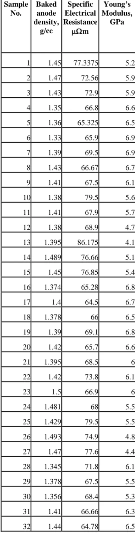
Table 2. Properties of baked anode samples Sample No. Baked anode density, g/cc Specific Electrical Resistance µΩm Young’s Modulus, GPa 1 1.45 77.3375 5.2 2 1.47 72.56 5.9 3 1.43 72.9 5.9 4 1.35 66.8 6.6 5 1.36 65.325 6.5 6 1.33 65.9 6.9 7 1.39 69.5 6.9 8 1.43 66.67 6.7 9 1.41 67.5 6.1 10 1.38 79.5 5.6 11 1.41 67.9 5.7 12 1.38 68.9 4.7 13 1.395 86.175 4.1 14 1.489 76.66 5.1 15 1.45 76.85 5.4 16 1.374 65.28 6.8 17 1.4 64.5 6.7 18 1.378 66 6.5 19 1.39 69.1 6.8 20 1.42 65.7 6.6 21 1.395 68.5 6 22 1.42 73.8 6.1 23 1.5 66.9 6 24 1.481 68 5.5 25 1.429 79.5 5.5 26 1.493 74.9 4.8 27 1.47 77.6 4.4 28 1.345 71.8 6.1 29 1.378 67.5 5.5 30 1.356 68.4 5.3 31 1.41 66.66 6.3 32 1.44 64.78 6.5 33 1.42 65.8 6 34 1.405 70.5 6.1 35 1.499 65.4 5.8 36 1.475 66.4 5.3

Table 3.Parameters for feed-forward neural network models used for prediction Property Electrical resistivity Young's modulus Baked anode density

Network newcf newcf newff

Transfer function

Layer 1 logsig logsig logsig

Layer2 purelin tansig purelin

Training

function trainlm trainlm trainlm

Learning

algorithm learngdm learngd learngd

Error

check mse mae mae

Initialization

Function rands rands rands

Seed for rands function

4 7 10

process the input to a layer such that the output can be easily classified into groups of similar data, which is important for an efficient prediction. Initially, some random weights were associated with the normalized input parameters. The training of a neural network means the identification of optimum values of the weights associated with the input parameters. The training of the network was done using trainlm, trainbfg, and traingdm back-propagation functions. Those functions were based on Levenberg-Marquardt, BFGS (Broyden, Fletcher, Goldfarb, and Shanno) update of quasi Newton, and gradient descent with momentum back-propagation algorithms, respectively. The maximum number of iterations for training (epoch) was set to 1000. The weights were varied during each iteration based on the gradient descent learning algorithms (learngd and learngdm) and a learning rate of 0.05 and momentum of learning of 0.9. The networks were trained based on the measurement of error in prediction. The errors were measured in terms of mean squared error (mse) and mean average error (mae). The 32 data set were used for the training of the neural network. The trained network was used to predict the properties of the baked anode for the four test data sets.

For all three cases, the predicted values were plotted against the published results for the four test data sets. The coefficient of determination for linear regression for each graph was used as the criteria for the quality of prediction. The closer the value of the coefficient of determination to unity is, the better the ability of prediction is.

(5)

Results and discussions

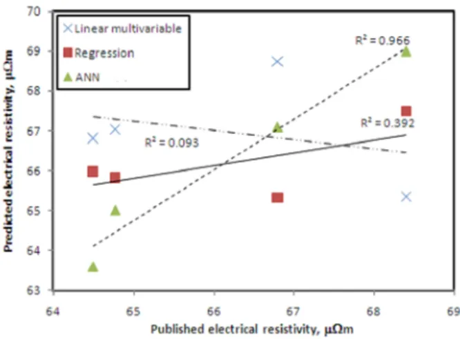
Figures 1, 2, and 3 show the correlation between the published and predicted values for electrical resistivity, Young’s modulus and baked anode density, respectively. The figures show that the coefficients of determination are the smallest (0.093, 0.332, and 0.604 for electrical resistivity, Young’s modulus, and baked anode density, respectively) in the case of linear multivariable analysis. The values for the coefficients of determination are medium (0.392, 0.846, and 0.816 for electrical resistivity, Young’s modulus, and baked anode density, respectively) in the case of regression analysis. The values are highest (0.966, 0.989, and 0.947 for electrical resistivity, Young’s modulus, and baked anode density, respectively) in the case of feed-forward ANN. For the feed-forward ANN, the configurations were different for the three cases. Table 3 lists the important parameters for the ANN models.

Figure 1. Predicted and published values of electrical resistivity

Figure 2. Predicted and published values of Young’s modulus

Figure 3. Predicted and published values of baked anode density Thus it can be seen that the customized feed-forward neural network model with back-propagation training was able to predict the output for the test data set better than the linear multivariable and regression analyses. The average percent errors in prediction are 0.8, 1.6, and 0.6 for electrical resistivity, Young’s modulus, and baked anode density, respectively.

In the production of anodes, there are numerous parameters that can influence the baked anode properties. Industries often maintain information about the input parameters and the output properties. These huge data can be utilized to train ANN. The industrial data is highly nonlinear in nature, and there is no mathematical relation available between those data. In such a situation, ANN has immense potential in quality control during anode production. In the case of variations in the properties of raw materials and processing parameters, ANN can predict the property of baked anode even before baking. In the case of variations in process parameters during the manufacturing of baked anodes, ANN could indicate the necessary changes in other process parameters to maintain the quality of baked anodes.

Conclusions

The artificial neural network is an important tool for the prediction of anode properties. It can become an important tool for the quality control of anodes. The major advantage of ANN over the other methods is that it can efficiently handle highly nonlinear data with noises where there is no existing mathematical relationship. It is true that the development of an efficient ANN model is time consuming because it needs lot of trials and errors; but once it is developed, it can predict results for which no experimental data is available. For the training of an ANN, availability of large sets of data is important; but this is generally not a limitation in the case of industries. ANN, with its power of artificial intelligence, can save time and money for the aluminum industry.

Acknowledgements

The technical and financial support of Aluminerie Alouette Inc. as well as the financial support of the National Science and

Engineering Research Council of Canada (NSERC),

Développementéconomique Sept-Îles, the University of Québec at Chicoutimi (UQAC), and the Foundation of the University of Québec at Chicoutimi (FUQAC) are greatly appreciated.

(6)

References

1. A. I. Berezin, P.V. Polaykov, O.O. Rodnov, V.A. Klylov, “Improvement of Green Anodes Quality on the Basis of the Neural Network Model of the Carbon Plant Workshop”, Light Metals, (2002), 605-608

2. R.S. Govindaraju, A. R. Rao, "Artificial Neural Networks: A Passing Fad in Hydrology?", Journal of Hydrologic Engineering, 5 (3) (2000), 225 – 226.

3. W.S. McCulloch, W. Pitts, "A Logical Calculus of Ideas Immanent in Nervous Activity", Bulletin of Mathematical Biophysics, 5 (1943), 115 – 133

4. M.R. Kaul, L. Hill, C. Walthall, "Artificial Neural Network for Corn and Soybean Yield Prediction", Agricultural Systems, 85(1) (2005), 1 - 18.

5. J. T. Connor, R. D. Martin, L. E. Atlas, "Recurrent Neural Networks and Robust Times Series Prediction", IEEE Transactions on Neural Networks, 5(2) (1994), 240 - 254.

6. Y. Hayashi, J. J. Buckley, E. Czogala, "Fuzzy Neural Network with Fuzzy Signals and Weights", International Joint Conference on Neural Networks, 2 (1992), 696 - 701.

7. X.Yao, "Evolving Artificial Neural Networks." Proceedings of the IEEE, 87(9) (1999): 1423 - 1447.

8. Z. R. Yang, "A Novel Radial Basis Function Neural Network for Discriminant Analysis", IEEE Transactions on Neural Networks, 17( 3) (2006), 604 - 612.

9. V. Cherkassky, J. H. Friedman, H. Wechsler, “From Statistics to Neural Networks”, Springer-Verlag, Berlin (1993).

10. J.K. Kruschke , J. R. Movellan. "Benefits of Gain: Speeding Learning and Minimal Hidden Layers in Back-Propagation Networks." IEEE Transactions on Systems, Man and Cybernetics.Vol. 21. No. 1 (1991): 273 – 280.

11. B. Cheng, D. M. Titterington, "Neural Networks: A Review from a Statistical Perspective", Statistical Science, 9(1) (1994), 2 - 30.

12. C.M. Zealand, D. H. Burn, and S. P. Simonovic, "Short Term Streamflow Forecasting Using Artificial Neural Networks", Journal of Hydrology, 214 (1999), 32 - 48.

13. J.W. Denton, "How Good are Neural Networks for Casual Forecasting?”, Journal of Business Forecasting, 14 (1995), 17 - 20.

14. H. White, “Artificial neural networks: Approximation and Learning Theory”, Blackwell, Cambridge, (1992).

15. G. Daqi, Y. Genxing, "Influences of Variable Scales and Activation Functions on the Performance of Multilayer Feedforward Neural Networks", Pattern Recognition, 36 (2003), 869 - 878.

16. A. Shigidi, L. A. Garcia, "Parameter Estimation in Groundwater Hydrology Using Artificial Neural Networks."

Journal of Computing in Civil Engineering, 17(4) (2003), 281 - 289.

17. W.S. Sarle, "Neural Networks and Statistical Methods", Proceedings of the Nineteenth Annual SAS Users Group International Conference, (1994).

18. V.R. Prybutok, J. Yi, D. Mitchell, "Comparison of Neural Network Models with ARIMA and Regression Models for Prediction of Houston's Daily Maximum Ozone Concentrations", European Journal of Operational Research, 122 (2000), 31-40. 19. C.X. Feng, X. Wang, "Surface Roughness Predictive Modeling: Nerual Networks Versus Regression", IIE Transactions, 35 (2003), 11 - 27.

20. J. Chmelar, “Size Reduction and Specification of Granular Petrol Coke with Respect to Chemical and Physical Properties”, (PhD Thesis, Norwegian University of Science and Technology, 1992).

21. D.F. Specht, "A General Regression Neural Network", IEEE Tras. Neural Networks, 2(6) (1991), 568-576.

22. P.D. Wasserman, "Advanced Methods in Neural Computing", Van Nostrand Reinhold, New York, (1993), 155-61