Attitude Control of an Underwater Vehicle
Subjected to Waves
by
CHRISTOPHER JOHN WILLY
B. S. Systems Engineering, United States Naval Academy (1981) Submitted in partial fulfillment of the requirements for the degrees of
OCEAN ENGINEER
at the
MASSACHUSET'IS INSTITUTE OF TECHNOLOGY and the
WOODS HOLE OCEANOGRAPHIC INSTITUTION and
MASTER OF SCIENCE IN MECHANICAL ENGINEERING at the
MASSACHUSETS INSTITUTE OF TECHNOLOGY
September 1994
© 1994 Christopher J. Willy. All rights reserved.
The author hereby grants to MIT and WHOI permission to reproduce and to distribute publicly paper and electronic copies of this thesis document in whole or in part.
Signature of Author ... . ... ...
Joint Program in Oceanographic Engineering, Massachusetts Institute of Technology and Woods Hole Oceanographic Institution, August 5, 1994
Certified by ... ...
Dr. Dana R. Yoefer, W s Hole Oeanygraphic Institution, Thesis Supervisor
Certified by ... ... .
Professor Michael S. Triantafyllou, Massachusetts Institute of Technology, Thesis Reader
ODE, I
Certified by ... ... . - ... -...
Professor Jean-Jagues E. Slotine, Massachusetts Institute of Technology, Thesis Reader
Accepted
by...
...
Professor Arthur B. Baggeroer, Chairperson, Jint Committee for Oceanograp Engineering Massachusetts Institute of Technology and the Woods Hole Oag .tit~ tion
Attitude Control of an Underwater Vehicle
Subjected to Waves
by
Christopher John Willy
Submitted to the Massachusetts Institute of Technology and Woods Hole Oceanographic Institution
Joint Program in Oceanographic Engineering
in August, 1994, in partial fulfillment of the requirements for the degrees of
OCEAN ENGINEER
and
MASTER OF SCIENCE IN MECHANICAL ENGINEERING
Abstract
This paper presents a method for estimating the spectra of water wave disturbances on
five of the six axes of a stationary, slender body underwater vehicle in an inertia dominated wave force regime, both in head seas and in beam seas. Inertia dominated wave forces are typical of those encountered by a 21 inch diameter, torpedo shaped underwater vehicle operating in coastal waters and sea state 2. Strip theory is used to develop transfer function phase and magnitude between surface water waves and the slender body pitch, heave, and surge forces and moment for the vehicle in head seas, and for pitch, heave, yaw, and sway forces and moments in beam seas.
Experiments are conducted which verify this method of transfer function calculation, and
demonstrate the effects of vehicle forward motion in the head seas case. Using known sea spectra and linear time invariant systems theory allows for estimation of the water wave disturbance spectra for these forces and moments.
Application of sliding control techniques are then developed for the underwater vehicle longitudinal plane equations of motion. Computer simulations are used to demonstrate the dependence of underwater vehicle depth control upon the pitch control, and adaptive pitch control is shown to provide good performance in the presence of substantial parametric uncertainty. Pitch disturbance rejection properties of variations of the sliding controller are investigated. Both single frequency and stochastic disturbances are used, and the stochastic disturbance is developed using the results of the earlier investigation.
Thesis Supervisor: Dr. Dana R. Yoerger Woods Hole Oceanographic Institution
Acknowledgements
The successful completion of this thesis was made possible through the support and
encouragement of my family, friends and colleagues. Special appreciation is due
Dana Yoerger Michael Triantafyllou Mike Hajosy Dan Leader Dave Barrett My Parents My Children Joan
my advisor, for his guidance, support, and unfailing encouragement
during these past two years,
for his frequently sought insight and advice,
for his perceptive ideas and our continuous dialogue,
for his friendship and example,
for his tremendous help and advice at the MIT tow tank,
who have always encouraged me in my every endeavor,
Nichole, Megan, Michael and Diana, for their patience and
understanding, and especially
my wife, who makes it all worthwhile.
The United States Navy is gratefully acknowledged for the graduate education
opportunity provided. This research was sponsored in part by ONR Contract
Table of Contents
Chapter 1 INTRODUCTION ... 13
1.1 M otivation ... 13
1.2 Research Objectives ... 14
1.3 Outline of Thesis ... 15
Chapter 2 WAVE DISTURBANCE ... 17
2.1 Linear Wave Results ... 17
2.1.1 Regular Waves ... 17
2.1.2 Statistical Description of Waves ... 19
2.2 Force Predictions ... 23
2.2.1 Load Regimes ... 23
2.2.2 Inertia Dominated Flow ... 26
2.2.2.1 Head Seas ... 26
2.2.2.2 Beam Seas ... 32
2.2.3 LTI Systems with Stochastic Inputs ... 38
Chapter 3 EXPERIMENTAL TESTING ... 41
3.1 Experimental Setup . ... 41...
3.1.1 Experimental Apparatus ... 41
3.1.2 AUV Mode l ... 43...
3.2 Testing ... 44...
3.2.2 Scaling Considerations ... 44 3.2.2.1 W ave Frequencies ... 44 3.2.2.2 AUV Speeds ... 46 3.2.3 Tests Conducted ... 48 3.3 Test Results ... 48 3.3.1 Raw Data ... 48 3.3.2 Signal Processing ... 51
3.3.3 Experimental Data vs. Theory ... 53
3.3.3.1 Stationary Model in Head Seas ... 53
3.3.3.2 Stationary Model in Beam Seas ... 61
3.3.3.3 Forward Moving Model in Head Seas ... 72
Chapter 4 AUV DYNAMICS ... 76
4.1 Equations of M otion ... 76
4.1.1 Coordinate Systems ... 76
4.1.2 Rigid Body Dynamics ... 80
4.1.3 Hydrodynamic Forces ... 82
4.1.4 Body Symmetry Considerations ... 85
4.2 Model Simplifications ... 87
Chapter 5 CONTROLLER DESIGN AND SIMULATIONS ... 90
5.1 Robust Sliding Contr ol .. ... 91
5.1.1 Over view ... 91
5.1.2 Application to 21UUV Longitudinal Plane Equations ... 94
5.2 Adaptive Sliding Control ... 97
5.2.1 Application to 21UUV Pitch Equation . ...97
5.3 Sim ulation Results ... 100
5.3.1 Additional Modeling Considerations ... ... ... 100
5.3.2 Depth Trajectory Following ... 103
5.3.3 Pitch Control in Regular W aves ... 119
5.3.4 Pitch Control in Random W aves ... 123
5.3.5 Summary ... 131
Chapter 6 CONCLUSIONS ... 133
6.1 Sum m ary ... 133
6.2 Future Directions ... 136
List of Figures
Figure 1.1 21UUV Profile ... 14
Figure 2.1 ITTC Spectrum for Seas not Limited by Fetch ... 23
Figure 2.2 Load Regimes on a Vertical Cylinder ... 25
Figure 2.3 Body-Fixed Axis, Force and Moment Conventions for a UUV ... 27
Figure 2.4 Heave Force Transfer Function Magnitude for 21UUV in Head Seas ... 31
Figure 2.5 Pitch Moment Transfer Function Magnitude for 21UUV in Head Seas ... 31
Figure 2.6 Surge Force Transfer Function Magnitude for 21UUV in Head Seas ... 32
Figure 2.7 Sway Force Transfer Function Magnitude for 21UUV in Beam Seas ... 36
Figure 2.8 Heave Force Transfer Function Magnitude for 21UUV in Beam Seas ... 36
Figure 2.9 Pitch Moment Transfer Function Magnitude for 21UUV in Beam Seas ... 37
Figure 2.10 Yaw Moment Transfer Function Magnitude for 21UUV in Beam Seas ... 37
Figure 2.11 LTI System ... 38
Figure 2.12 Pitch Disturbance Spectrum for 21UUV in Head Seas ... 40
Figure 2.13 Two Possible Time Realizations of Pitch Disturbance ... 40
Figure 3.1 Experimental Apparatus Setup ... 42
Figure 3.2 21UUV Model Used in Testing ... 42
Figure 3.3a Sample of Surge Force and Roll Moment Raw Data ... 49
Figure 3.3b Sample of Sway Force and Pitch Moment Raw Data ... 50
Figure 3.3c Sample of Heave Force and Yaw Moment Raw Data ... 50
Figure 3.4 Frequency Response of Filter ... 52
Figure 3.5 Two Samples of Unfiltered and Filtered Signals ... 53
Figure 3.6a Surge Force Transfer Function Magnitude for Shallow Model in Head Seas ...55
Figure 3.6b Surge Force Transfer Function Phase for Shallow Model in Head Seas ... 55
Figure 3.7a Heave Force Transfer Function Magnitude for Shallow Model in Head Seas ... 56
Figure 3.7b Heave Force Transfer Function Phase for Shallow Model in Head Seas ... 56
Figure 3.8a Pitch Moment Transfer Function Magnitude for Shallow Model in Head
Seas
...
57
Figure 3.8b Pitch Moment Transfer Function Phase for Shallow Model in Head Seas ... 57
Figure 3.9a Surge Force Transfer Function Magnitude for Deep Model in Head Seas ... 58
Figure 3.9b Surge Force Transfer Function Phase for Deep Model in Head Seas ... 58
Figure 3.10a Heave Force Transfer Function Magnitude for Deep Model in Head Seas ...59
Figure 3.10 b Heave Force Transfer Function Phase for Deep Model in Head Seas ... 59
Figure 3.1 la Pitch Moment Transfer Function Magnitude for Deep Model in Head Seas ... 60
Figure 3.1 lb Pitch Moment Transfer Function Phase for Deep Model in Head Seas ...60
Figure 3.12a Sway Force Transfer Function Magnitude for Shallow Model in Beam
Seas
...
62
Figure 3.12b Sway Force Transfer Function Phase for Shallow Model in Beam Seas ... 62
Figure 3.13a Heave Force Transfer Function Magnitude for Shallow Model in Beam S eas ... ... 3
Figure 3.13b Heave Force Transfer Function Phase for Shallow Model in Beam Seas ... 63
Figure 3.14a Roll Moment Transfer Function Magnitude for Shallow Model in Beam
Seas
...
64
Figure 3.15a Pitch Moment Transfer Function Magnitude for Shallow Model in Beam
Seas ... 65
Figure 3.15b Pitch Moment Transfer Function Phase for Shallow Model in Beam Seas ... 65
Figure 3.16a Yaw Moment Transfer Function Magnitude for Shallow Model in Beam S eas ... 66
Figure 3.16b Yaw Moment Transfer Function Phase for Shallow Model in Beam Seas ...66
Figure 3.17a Sway Force Transfer Function Magnitude for Deep Model in Beam Seas ...67
Figure 3.17b Sway Force Transfer Function Phase for Deep Model in Beam Seas ... 67
Figure 3.18a Heave Force Transfer Function Magnitude for Deep Model in Beam Seas. ...68
Figure 3.18b Heave Force Transfer Function Phase for Deep Model in Beam Seas ... 68
Figure 3.19a Roll Moment Transfer Function Magnitude for Deep Model in Beam Seas ... 69
Figure 3.19b Roll Moment Transfer Function Phase for Deep Model in Beam Seas ... 69
Figure 3.20a Pitch Moment Transfer Function Magnitude for Deep Model in Beam Seas ...70
Figure 3.20b Pitch Moment Transfer Function Phase for Deep Model in Beam Seas ... 70
Figure 3.21 a Yaw Moment Transfer Function Magnitude for Deep Model in Beam Seas ... 71
Figure 3.2 lb Yaw Moment Transfer Function Phase for Deep Model in Beam Seas ... 71
Figure 3.22 Surge Force Transfer Function Magnitude for Model at 0.489 m/s in Head
Seas
...
73
Figure 3.23 Heave Force Transfer Function Magnitude for Model at 0.489 m/s in Head Seas ... 73
Figure 3.24 Pitch Moment Transfer Function Magnitude for Model at 0.489 m/s in Head Seas ... 74
Figure 3.25 Surge Force Transfer Function Magnitude for Model at 0.733 m/s in Head
Seas
...
74
Figure 3.26 Heave Force Transfer Function Magnitude for Model at 0.733 m/s in Head
Seas ... ... 75
Figure 3.27 Pitch Moment Transfer Function Magnitude for Model at 0.733 m/s in Head Seas ... ... 75
Figure 4.1 The Euler Angles ... 77
Figure 5.1 Sternplane and Thruster Dynamics Model ... 101
Figure 5.2 21 UUV Depth Trajectory with Robust Sliding Pitch Controller ... 105
Figure 5.3 21UUV' Pitch Response During Depth Maneuver ... 106
Figure 5.4 21 UUV Speed Response During Depth Maneuver ... 107
Figure 5.5 Robust Sliding Pitch Controller keff (t) ... 108
Figure 5.6 21UUV Depth Trajectory with Adaptive Sliding Pitch Control Law, r = 0... 109
Figure 5.7 21UUV Pitch Response with Adaptive Sliding Pitch Control Law, F = 0 ... 110
Figure 5.8 21UUV Depth Trajectory with Adaptive Sliding Pitch Control Law, F = ... O ... 111
Figure 5.9 21UUV Pitch Response with Adaptive Sliding Pitch Control Law, r = 0... 112
Figure 5.10 Adaptation of and s with ... ... 113
Figure 5.11 21UUV Depth Trajectory with Adaptive Sliding Pitch Control Law, F = 0 ... 114
Figure 5.12 21UUV Pitch Response with Adaptive Sliding Pitch Control Law, = 0 ... 115
Figure 5.13 21UUV Depth Trajectory with Adaptive Sliding Pitch Control Law, F = ... 116
Figure 5.14 21UUV Pitch Response with Adaptive Sliding Pitch Control Law, r = ... ... 117
Figure 5.15 Adaptation of and sowith ... 118
Figure 5.16 Adaptive Pitch Control Law with Single Frequency Disturbance, = 0 ... 120
Figure 5.17 Adaptive Sliding Pitch Controller with Single Frequency Disturbance ... 121
Figure 5.18 Adaptation to a Single Frequency Disturbance by the Pitch Controller ... 122
Figure 5.19 Wave Disturbance Spectra . ... 124
Figure 5.21 Adaptive Sliding Pitch Control with Stochastic Disturbance ... 1 26 Figure 5.22 Adaptive Sliding Pitch Control with Stochastic Disturbance ... 127 Figure 5.23 Adaptive Sliding Pitch Control with Stochastic Disturbance ... 129 Figure 5.24 Adaptive Sliding Pitch Control with Stochastic Disturbance ... 130
List of Tables
Table 3.1 Frequencies and Wavelengths Investigated During Testing ... 47
Table 3.2 Tow Speeds Investigated During Testing ... 47
Table 3.3 Summary of Tests Conducted ... 48
Table 4.1. SNAME Notation Used for Ocean Vehicles ... 79
Chapter 1
INTRODUCTION
1.1 Motivation
Autonomous Underwater Vehicles (AUVs) have become increasingly useful tools in the
exploration of the ocean depths, where the effects of surface waves are far removed from the
operating region of the vehicle. As the range of missions for AUVs expands, so does the need to
understand the disturbances which the vehicle will encounter in its enlarged theater of operation.
While deep underwater, ocean currents may be the source of the predominant disturbance to the
untethered AUV, the effect of gravity water waves becomes important when operating an AUV
near the water's surface.
The Naval Undersea Warfare Center (NUWC) Division, Newport, Rhode Island, is
currently developing an autonomous, 21 inch diameter "torpedo shaped" AUV, known as the
21UUV, for which near surface operations is envisioned in the future. The 21UUV shape, in the
expected 301 inch long version, is shown in figure 1.1.
The Deep Submergence Laboratory at the Woods Hole Oceanographic Institution is
involved in the research and development of the control algorithms for the vehicle, and an
understanding of the expected environmental disturbances to the AUV will allow a more thorough
evaluation of the effectiveness of the developed controllers. Also, future decisions concerning
possible operating regions of the 21 UUV must account for water surface conditions and the effect
301 in
20.94 in
Figure 1.1 21UUV Profile
1.2 Research Objectives
In severe sea conditions, the destabilizing effect of surface waves on an AUV is expected
to be the limiting factor when considering the upper boundary of useful operating depths
available to the underwater vehicle. For example, with surface waves in deep water, one would
expect the amplitude of water motion, and hence the effect of wave forces, to decay with
increasing depth. Because there is a limit in its ability to stabilize itself, an AUV would have a
ceiling to its effective operating regime. Therefore, one reasonable measure of an AUV controller
is its performance in the presence of wave disturbances.
Before the disturbance rejection properties of any controller can be evaluated, the
properties of the disturbance must be determined. Because the 21UUV shape is relatively simple,
existing literature concerning the hydrodynamic forces on similar shaped bodies, i.e. cylinders, is
abundant. Therefore the first objective of this thesis is to apply existing theory to develop a
model for predicting the forces and moments caused by sea waves on a stationary, slender body
AUV. Linear wave theory, hydrodynamic strip theory accounting for the precise contour of the
With any model, simplifications of the true physical processes result in model
inaccuracies. While full scale testing of the yet to be built 21UUV is beyond the scope of this
thesis, scale model testing in a wave tank is possible. Therefore, the second research objective is
to conduct tests which either confirm the validity of the wave force and moment model, or
provide empirical data which allows for the estimation of the hydrodynamic forces and moments
on the AUV.
While a precursor of the 21UUV is currently undergoing sea trials which, in part, are
being used to evaluate controller performance in still water and in steady currents, the testing of
this vehicle in other than calm sea conditions is a future prospect. Hence, the third research
objective is to develop a controller for the 21UUV using the same methodology as is expected to
be used for the actual 21UUV controller, and by simulation, to evaluate the controller's
performance in the presence of wave disturbances similar to that which might be encountered in
practice. For simplification purposes, motion in the AUV's longitudinal plane alone is
considered.
1.3 Outline of Thesis
Chapter 2 develops theory allowing for the estimation of wave disturbances on a
stationary slender body AUV beneath the water's surface. Slender body strip theory and linear
wave theory are used to develop a method for calculating the transfer function phase and
magnitude between surface water waves and five of the six forces and moments expected for the
submerged AUV, both in head and in beam seas. A spectral description of random water waves
is presented, and using linear time invariant systems theory, a method for calculating the spectra
of the wave disturbance is shown. Generating a time simulation of waves from their spectral
Chapter 3 contains a description of the experimental testing performed on a scale model
of the 21UUV to evaluate the transfer function representation of wave forces and moments
presented in chapter 2. The experimental apparatus is detailed, as are the series of tests
performed. Experimental data is compared to theoretical values and largely verifies the earlier
developed theory. The effect on transfer function magnitude of vehicle forward motion in head
seas is also investigated. Differences and similarities between the static and dynamic model cases
are noted.
Chapter 4 details the general six degree of freedom equations of motion for an
underwater vehicle. Model simplifications are made accounting for 21UUV body symmetry and
assumptions concerning maintenance of the vehicle roll angle at 0 degrees. The resulting
longitudinal plane equations used for subsequent discussion are presented.
Chapter 5 provides a method of applying sliding control techniques to the 21UUV in the
longitudinal plane. Variations of the sliding controller are applied to the vehicle pitch axis, and
are demonstrated in simulation as an integrated part of the pitch-depth-speed controller. Pitch
disturbance rejection properties of the controllers is investigated through time simulations, and
extensions to an adaptive sliding controller are made in an attempt to improve disturbance
rejection properties.
Chapter 6 summarizes the results of the thesis and describes the direction of future
Chapter 2
WAVE DISTURBANCE
The results of linear wave theory provide a first order approximation to the motion of a
body of water due to surface gravity waves. Some results from the theory are presented here, and
then are used to develop a model of the stochastic disturbance which could be expected to affect
an AUV operating near the surface of the ocean, where the wave effects are most prominent.
This wave disturbance model will be compared to experimental results in a later chapter, and then
used in AUV dynamic simulations, where the goal will be to reduce the effect of wave
disturbances through the use of different control schemes.
2.1 Linear Wave Results
A more thorough discussion of these results can be found in (Newman 1977), or
(Faltinsen 1990).
2.1.1 Regular Waves
For a single frequency water wave traveling in the direction measured by the angle a
with respect to the Cartesian coordinate frame positive x direction, the free surface elevation
above the mean free surface can be described by
where 5, represents the surface wave amplitude (half the wave height), o = 2' is the circular frequency, T is the wave period, t is time, k= -A is the wave number, and X is wavelength.
Wave number, k, is related to circular frequency, o, through the dispersion relation
' = k tanh kh (2.2)
where g is the acceleration of gravity, and h is the water depth (from mean free surface to ocean
floor).
For a wave traveling from one water depth to another, o remains constant, and the wave number, and therefore the wavelength are affected by the change in h.
Assuming from here on that a = 0, a water particle's vertical motion, of amplitude , on
the surface, decays with depth, z, where z is taken positive down, and is described by
r
= , sinhk(-z+h) sinhkh sin(ot - kx) (2.3)while the water particle's horizontal motion is
_
= -cosh ,-zh) cos(tt - kx) (2.4)
The vertical velocity and acceleration fields are
W = )a sinhk(-z+h) cos(t - kx) (2.5)
a3 = - a sinhk-z+h)
sin( t-
kx)(2.6)
U =t coshk(-zh) sinhkh siin(tt - kx) (2.7)
a, = 2 coshk(-z+h) COS(t - kx) (2.8)
The dynamic pressure field in the water column is
PD = pg, cosh k(-z+h) sin (w t - kx) (2.9)
where p is the water density and g is the acceleration of gravity.
2.1.2 Statistical Description of Waves
In practice, linear wave theory is used to simulate irregular seas by the superposition of a
large number of regular waves (Faltinsen 1990). For a long crested, irregular sea with waves
traveling in the positive x-direction, the sea surface elevation can be described
N
; = A, Aj
sin(o t - kx
+2j)
i=i sin~roitk~rta j (2.10)
j=1
where Aj, j, k, and £j are the wave amplitude, circular frequency, wave number, and random
phase of the j-th wave component respectively, and N is the number of wave components used in
the simulation. The random phase angles are uniformly distributed between 0 and 27r radians,
and the wave number and circular frequency are related through the dispersion relation. Wave
amplitude is related to the circular frequency through a single-sided wave amplitude spectrum,
S+(to), and can be calculated from
Here, Ato is the increment in to used in the discrete approximation of the spectrum S+(o). In
implementing equation (2.10), oj is chosen randomly and uniformly in the interval oi to oi + Ao
= oi,+ to avoid the repetition of the expression after 2/Aco seconds. It follows that the horizontal
velocity and acceleration fields, and the vertical velocity and acceleration fields can be simulated
in the same manner, as
cojAj
coshkj(-z+h) sin(ot-
kjx+£j)
(2.12)i=1
a,
sinhkih
cos(t - kx
+ )
(2.13)
j=N = sinhkjhw
hkh-
cos(o,
t-kx+ )
(2.14)
j=1NW -
tj2Aj
sinhkj(-z+)sin(ot sinhk jh- kjx + j)
(2.15)
j=l
respectively, and that the dynamic pressure can be simulated byN
PD = py A cosh ki (-z+h)
)
cpa3 o 2 ihkjt-zh k sin(ot-kjx+Ej ) (2.16)
j=1
The single-sided spectrum S+(co) is commonly used in Ocean Engineering applications,
and is defined
S+(co)
=DT;('t)e-J d'
0
(2.17)
where
(t)= lim
J
(t)
(t +
)
dt
(2.18)
-Y (2.18)
= E{(t) r(t + )}
is the sea surface elevation autocorrelation function. It can be recognized that S+(o) is related to
the familiar definition of the power spectrum, c, (co) (the Fourier transform of the autocorrelation function) as
S+(o) = ) (2.19)
O o<0
S+(o) can be calculated in the method described above, that is, by first calculating the
autocorrelation function of a set of wave data and then computing its Fourier transform. The
assumption made is that sea waves can be described as a stationary random process over some
short period of time on the order of a few hours. By curve fitting some function of frequency to
the resulting empirical data, many oceanographers have compactly described the frequency
content of their data by an empirical formula representing a continuous wave spectrum (St. Denis
1969).
The forms of the function used to curve fit wave record data to describe a spectrum are
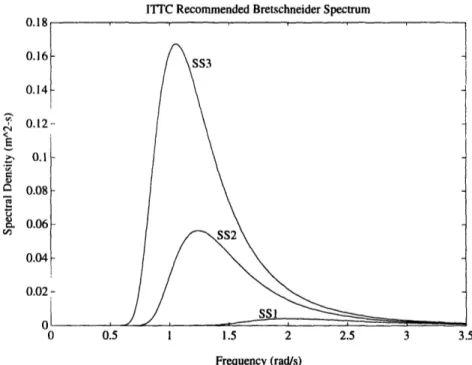
various. Bretschneider is credited with proposing the first easily usable two parameter spectrum
representing seaways in all states of development (Chryssostomidis 1974). The 15th
International Towing Tank Conference (ITTC) recommended a spectrum of the Bretschneider
a specific region of the seas is not available. For seas not limited by fetch, the ITTC
recommended Bretschneider spectrum has the form
173HI
(-691~
S+()= 14 5 exp ) T (2.20)
Here, Tlis the average wave period, and Ha is the significant wave height, defined as the average
of the highest one third of all the waves (15th ITTC 1978).
The term "sea state" is commonly used to describe sea surface conditions ranging from
glassy seas (sea state 0) to those encountered during hurricane conditions (sea state 9). Using
data published in (Berteaux 1991) relating sea states to the two parameters above, the ITTC
recommended spectrum for conditions spanning sea states 1 through 3 is depicted in figure 2.1.
It can be seen that as the sea state becomes rougher, the spectrum becomes more peaked, and the
modal frequency decreases. Also, the majority of the spectrum power is seen to be in frequencies
below 3 rad/sec, even for the calmest of seas.
The ITTC recommended spectrum will be selected as the sample wave spectrum in all
following discussion and simulations. While this spectrum may not be the best available model
of the actual wave spectrum for a specific application, it is assumed to be sufficiently
ITIC Recommended Bretschneider Spectrum S 1I.E -IV c En .5 Frequency (rad/s)
Figure 2.1 ITTC Spectrum for Seas not Limited by Fetch and Conditions Ranging from Sea States 1 to 3
2.2 Force Predictions
2.2.1 Load RegimesMorison was the first to propose that the horizontal force per unit length on a stationary
vertical cylinder in waves can be written as
dF = (p- CMa +p
CDulul)dl
(2.21)where p is the water density, D is the cylinder diameter, I is the cylinder length, a and u are the
horizontal acceleration and velocity of the water at the depth of the cylinder section, and CM and
CD are coefficients which can be determined experimentally (Morison, et al 1950). It is seen that
representing an inertial force proportional to the acceleration of the water at the depth of interest,
and a second, nonlinear drag term proportional to sign velocity times square velocity of the water
at the depth of interest. In practice, CM and CD are dependent on several parameters such as the
Reynolds and Keulegan Carpenter numbers of the flow, and the surface roughness of the
cylinder.
It is therefore possible that in a particular type of flow that either the inertia or drag force
is predominant. Such is the case for vertical pilings penetrating the water's surface, and it is
known that the ratios of wavelength and waveheight to cylinder diameter are key parameters in
predicting the load regime of the waves on the cylinder (Faltinsen 1990). Figure 2.2 depicts these
load regimes.
For a stationary object in a simple harmonic oscillating flow, the time varying total force
can then be expressed as
F, = FD sin otlsin ot[+ F, cosot (2.22)
where FD and Fl represent the maxima of the drag and inertia force components, respectively. It
can be shown that (Dean and Dalrymple 1984)
F, 2FD < F,
FT
FD +=
F 2FD > Fl (2.23)D·-ja.
4F,F
2Fo>
The significance of equation (2.23) is that the maximum force on the body is not affected
by additional drag force until the amplitude of the drag is at least one half that of the inertia
force. For harmonic oscillating flows, such as that caused by regular waves, while even small
Load Regimes 102 (4) Drag Dominan 10' No Waves 90% drag > ---i --- --... (3) Morison 10-1 /' (2) Inertia Dominant (1) Diffraction mportant 10-2 ' 10-1 100 101 102 103 Lambda / D
Figure 2.2 Load Regimes on a Vertical Cylinder (Adapted from (Faltinsen 1990))
stationary body, the peak amplitude of the force is only affected when the drag component is
greater than one half the inertia force. This implies that if the peak of the regular wave force is
the main concern for a particular submerged body, considering figure 2.2, water particle motion
with amplitude greater than 0.5 diameters, and perhaps up to 2.5 diameters would produce a peak
force only as high as the peak force due to the inertia term from equation (2.22).
The same concepts discussed above will be used to predict the predominant forces on a
stationary horizontal cylindrical body (the 21UUV) under waves. When waves cause the motion
of a water particle at an AUV's depth to be of the order of one UUV diameter or less, it is
expected that the predominant hydrodynamic force on the UUV due to the wave disturbance
would be inertial in nature. Because an AUV may be deeply submerged, it is not the surface
wave height to AUV diameter ratio which is of concern, but more appropriately twice the
to wave height) compared to the cylinder diameter. For instance, if yaw moment on the body is
of concern, horizontal water motion tangent to the longitudinal (x) axis of the AUV should be
considered as this is the flow which causes the yaw moment.
While the above analogy is approximate in nature, it provides a means to predict which
hydrodynamic forces may be of concern when predicting the total load on a cylindrical AUV
caused by waves. Experimental data will be presented in a later chapter which tests the validity
of these arguments.
2.2.2 Inertia Dominated Flow
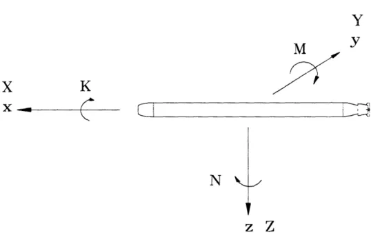
Figure 2.3 depicts the axes, force and moment conventions for an AUV used in this and
subsequent discussions. The body-fixed axes are labeled x, y, and z, with forces X, Y, and Z
positive in the corresponding positive axis direction, and moments K, M, and N are positive using
the right hand rule.
For the long, streamlined body of the 21UUV, strip theory can be used to calculate the
hydrodynamic forces and moments imposed on the stationary body by water flow perpendicular
to the longitudinal axis of the body. Considered below are two body-to-wave orientations, both
for the horizontal vehicle in an inertia dominated wave force regime. Strip theory is first applied
to estimate the heave force, Z, the pitch moment, M, and the surge force, X, on the vehicle in
direct head seas, where wave propagation is perpendicular to the AUV longitudinal axis. Then Y
(sway force), Z, M, and N (yaw moment) are estimated for the vehicle in direct beam seas, i.e.,
when wave propagation is parallel to the vehicle longitudinal axis.
2.2.2.1 Head Seas
To better understand what to expect for Z and M on the AUV body under head seas, first considered is a right cylinder of constant diameter equal to the maximum diameter of the 21 UUV,
Y
M
Y
x
K
X-
-~
-I
C__-Z
Figure 2.3 Body-Fixed Axis, Force and Moment Conventions for a UUV
and of the same length as the vehicle. Considering the nearly cylindrical shape of the 21UUV,
this cylinder model allows for a closed-form solution which roughly approximates the more
refined solution developed later using numerical methods and taking into account the precise body
contour of the AUV.
The vertical force (positive downward) on a stationary horizontal cylinder of length L
under waves traveling in the negative x direction in an inertia dominated force regime is
calculated here using strip theory as
ZH(t)=- KM3a3(x Z t) d
(2.24)
L
where KM3 = 7cpD
2
CM. To determine CM, the Keulegan-Carpenter parameter is considered and
is found for vertical water motion as
KC = wm T/D (2.25)
where
Wm = Ae sinhk(-z+h)
(2.26)
is the amplitude of the vertical velocity from equation (2.5), and T is the period of the harmonic
wave. It is seen that
KCv = 22t~m/D (2.27)
where m is the maximum vertical displacement of the water particle from its neutral position. It
is the assumption here that m/D, the "displacement" parameter, is 1 or less and that the resultant
hydrodynamic force is inertia dominated with CM - 2 (Dean and Dalrymple 1984).
Returning to equation (2.24), vertical water particle acceleration is taken at the centerline
depth of the cylinder. Using linear wave theory and recalling that the wave is now traveling in the
negative x direction, a3(x, z, t) taken from equation (2.6) can be expressed
a3(x, z, t) = A3(z)sin(kx + cot) (2.28)
Then, recalling that the force Z is taken positive down while the wave elevation is taken positive
up, L/2 ZH(t) = -KM3A3 sin(kx +
cot)dx
-L/2 (2.29) = -KM3A3 sin sin ( t) andSimilarly, M about the mid-length position on the same stationary horizontal cylinder
under the same waves is calculated using strip theory as
L/2
MH(t)= KM3A3
fxsin(kx + cot)dx
(2.31)
-L/2
= K3A3 (2 sin - kL cos)cos
cot
and|M
I=-
V (2sin
k - kL cos k)(2.32)
The surge force, X, can be estimated by calculating the difference in force between theback and front ends of the cylinder due to the difference in the undisturbed dynamic pressure:
XH(t) = -½ 3pgD 2 , coshk(-z+h) sin cos(ct)
IXHI
= pgD,,
coshk(-z+h) sin k(2.33)
For a given AUV depth in the water column, the above formulation relates wave number,
k, to the magnitude of Z, M, and X for unit amplitude surface waves. Since wave frequency is
directly related to wave number by the dispersion relation (equation (2.2)), equations (2.29),
(2.31), and (2.33) can be used to solve for the magnitude and phase of the transfer function from
to Z, M, and X.
For a more refined estimate of Z, M and X, the cylinder model of the 21UUV is
abandoned and the precise body contour of the AUV is accounted for. Then, from equation
(2.24),
L/2
ZH(t) =-A
3KM
3(x)sin(kx
+wt)dx
(2.34)
where KM3(x)= -:pxCMD2(x). CM -2 and constant is still assumed, and using numerical
methods with a look-up table for D(x), the amplitude of ZH can be found for all o and arbitrary
phase. Similarly,
L/2
MH(t) = A3 x KM3(x)sin(kx + ot)dx (2.35)
-L/2
where the same method can be used to find the amplitude for MH for all o and arbitrary phase.
Calculating X requires the integration of the dynamic pressure over the vehicle contour at both
ends, namely
R R
XH(t) =
27f
PD(Xtail(r))rdr - 2J PD(Xnose,(r))rdr (2.36)0 0
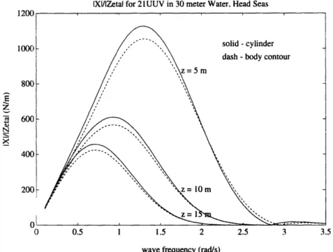
As examples of the calculated transfer function magnitudes, figures 2.4, 2.5, and 2.6 compare predicted |ZH(co)1/;,,a(co), IMH(o)j1/;a(co)I and IXH(oI))/I;a((o) for the 21UUV in head
seas, 30 meter deep water and at various depths using the two methods described above.
Figures 2.4, 2.5, and 2.6 show decreased transfer function magnitudes with increased
depth of the cylinder, as would be expected due to the decay of water motion with depth. Also
observed in these figures is a shift of the peak of the magnitude of the transfer functions to lower
frequencies with increased depth of the vehicle. This can be explained by realizing that higher
frequency waves decay more rapidly with increasing depth in the water column than do lower
IZI/IZetal for 21 UUV in 30 meter Water, Head Seas -Z V N N 5 wave frequency (rad/s)
Figure 2.4 Heave Force Transfer Function Magnitude for 21UUV in Head Seas
IMI/IZetal for 21UUV in 30 meter Water, Head Seas
z
N
"E:
0 0.5 1 1.5 2 2.5 3 3.5
wave frequency (rad/s)
Figure 2.5 Pitch Moment Transfer Function Magnitude for 21UUV in Head Seas OL
IXI/IZetal for 21UUV in 30 meter Water, Head Seas
E
N
0 0.5 1 1.5 2 2.5 3 3.5
wave frequency (rad/s)
Figure 2.6 Surge Force Transfer Function Magnitude for 21UUV in Head Seas
2.2.2.2 Beam Seas
In left beam seas, the AUV longitudinal axis is considered to be rotated 90° from the
incoming wave direction, and referring to figure 2.3, the regular wave propagation direction is
taken in the positive y direction in the body-fixed coordinate system. Considering the range of wavelengths over the range of wave frequencies which are of interest, it is noted that X/D > 13
for all wave frequencies below 3 rad/sec, and the approximation of uniform water acceleration
across the diameter of the AUV is made. Strip theory then allows for the calculation of Y, Z, M,
and N for the AUV in beam seas, while the roll moment, K, though expected to be of
significance, cannot be reasonably calculated in this manner. Experimental methods best allow
for determination of K in beam seas, and these will be explored in a later chapter.
Because Y and N are caused by horizontal water motion, the Keulegan-Carpenter
KCh = 2nmlD (2.37)
where
cash k (-z+h)2.8)
4m
sinhkh(2.38)
Here the horizontal displacement parameter m/D < 1 resulting in inertia dominated
hydrodynamic forces and CM - 2 is assumed.
Where the previously used cylinder model of the 21UUV can be used to calculate Y and
Z, using this approach to calculate M and N would predict zero moment about the mid length
position of the AUV, and therefore only the body contour method is used to calculate M and N in
beam seas.
Using the two methods previously described,
YB(t) = A2KM2Lcosot (2.39)
using the cylinder model of the body, or
L/2
Ys(t)=A
2coscot KM
2(x)dx
(2.40)
-L2
using the body contour of the vehicle to calculate KM2(x). Here A2 = A1 and is taken from
equation (2.8), KM2= KM3 and KM2(x) = KM3(x) due to the symmetry of the vehicle. Similarly,
Z is calculated
or
L2
ZB(t) =-A3 sin ot
J
KM3(X)dx (2.42)-L/2
for the cylinder model and body contour model, respectively.
The moments M and N are found from
L2 MB(t)=
A
3sinot x K,(x)dx
(2.43)
-L2 and L/2NB(t)= A
2cosot x KM
2(x)d
(2.44)
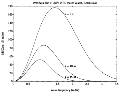
-L/2 respectively.Figures 2.7 through 2.10 show examples of the calculated transfer function magnitudes for IYB()j/|Ia(@O)|I IZB(CO)IIC(O))I IMB(o)I/Ita(o), and INB(@)j/ra.(@)I, respectively for the
21UUV in beam seas, 30 meter deep water and at various depths using the methods described
above. Comparing figures 2.7 and 2.8, the transfer function magnitudes are identical for the Y
and Z forces except at low frequencies where, because of the larger wavelength to water depth
ratio, the water particle motion decays more rapidly with depth for the vertical motion than for
horizontal water particle motion. The same can be said when comparing the M and N moments
in figures 2.9 and 2.10. Because there is little fore-aft asymmetry in the 21UUV, the predicted
pitch and yaw moments in beam seas are seen to be relatively small compared to the predicted
pitch moment in head seas (figure 2.5). Finally, comparing ZH in head seas versus ZB in beam
functions are identical. At higher frequencies where the wavelength is shorter and of the order of the vehicle length,
IZHl/llI
is predictably smaller thanIZBl/IUl.
The application of strip theory in calculating forces and moments on an AUV in head and
beam seas in an inertia dominated hydrodynamic force regime has allowed for the prediction of
the transfer function from surface wave amplitude to forces and moments on the AUV. The
standing assumption has been that water particle motion at the depth of the AUV is small enough
so that nonlinear hydrodynamic form drag is insignificant when compared to the linear
IYI/IZetal for 21UUV in 30 meter Water, Beam Seas
0 - 0.5 1 1.5 2 2.5 3 3.5
wave frequency (rad/s)
7 Sway Force Transfer Function Magnitude for 21 UUV in Beam
IZI/IZetal for 21 UUV in 30 meter Water, Beam Seas
a z N N Seas 0 0.5 1 1.5 2 2.5 3
wave frequency (rad/s)
Figure 2.8 Heave Force Transfer Function Magnitude for 21UUV
3.5
in Beam Seas
-N
IMI/IZetal for 21UUV in 30 meter Water, Beam Seas
z
N =:Z 2 160 140 120 100 80 60 40 20 0 0 0.5 1 1.5 2 2.5 3 3.5wave frequency (rad/s)
Figure 2.9 Pitch Moment Transfer Function Magnitude for 21UUV in Beam Seas
INI/IZetal for 21UUV in 30 meter Water, Beam Seas
E
-N
z
5 wave frequency (rad/s)
Figure 2.10 Yaw Moment Transfer Function Magnitude for 21UUV in Beam Seas
1n_
2.2.3 LTI Systems with Stochastic Inputs
Figure 2.11 depicts a linear time invariant (LTI) system with stable, proper transfer function G(s), input u(s), and output y(s), where s = ( ) is the Laplace operator.
u(s)
G(s)
y(s)
Figure 2.11 LTI System
Such systems have long been studied, and presented below is a well-known result which will be
used in later discussions. For a thorough treatment of the subject of LTI systems with stochastic
inputs, the reader can consult (Papoulis 1984), wherein the proof of the following result is
contained.
For the system in figure 2.11, if u(t) is a known input, and G(t), the impulse response of
the transfer function G(s) is known, then y(t) is known and can be expressed
y(t) = y(O) + u(x)G(t-
t)dx 0(2.45)
Considering the case when u(t) is a stationary, random process with known power
spectrum, then y(t) is also a stationary, random process. The power spectrum of y(t) can be
calculated as
(Pyy(o)) = IG(jto)l2 U (cO ) (2.46)
i
! I
where IG(jto)I is the magnitude of the transfer function G(s) evaluated at s = jo. It follows then,
that the single-sided spectrum of y(t), from equation (2.19) is
S
(
° 'o)=
(2.47)The significance of the above result is that the previous discussion relating surface wave
action to forces and moments on an AUV has been cast in such a framework. It can be seen that
if the magnitude of the transfer functions between sea surface waves and forces and moments on
an AUV are known, then the statistics of the forces and moments on the AUV body can be
determined.
As an example, the pitch disturbance spectrum on the 21UUV in head seas and sea state
2 conditions are calculated for various depths of the vehicle and depicted in figure 2.12. In
generating these spectra, the ITTC recommended Bretschneider wave amplitude spectrum for sea
state 2 was used, as well as the body contour generated transfer function from wave amplitude to
pitch disturbance depicted in figure 2.5.
Figure 2.13 depicts two possible time realizations of this pitch disturbance which are
generated using the technique described in section 2.1.2 for generating time realizations of
surface waves. The differences between the two realizations are due to the random phase used in
each simulation. There are, of course, an infinite number of possible realizations of this pitch
Pitch Disturbance Spectrum for 21UUV, Head Seas, SS2
0 0.5 1 1.5 2 2.5 3 3.5
Frequency (rad/s)
Pitch Disturbance Spectrum for 21UUV for Sea State 2 and at Various Depths
in Head Seas Time (sec)
z
0Z o0 [. 0 10 20 30 40 50 60 Time (sec)Figure 2.13 Two Possible Time Realizations of Pitch Disturbance to 21UUV in Head Seas, Sea State 2 and at 10 Meters Depth E: v. -c s a U1 Figure 2.12 '6
i
z
I-x 105Chapter 3
EXPERIMENTAL TESTING
In this chapter, experiments which test the theory of chapter 2 are discussed, and results
of tests conducted on a 21UUV model are presented and compared with the earlier developed
theory. While chapter 2 theory deals with forces on a stationary body, the wave forces on a
forward moving AUV are also of interest as many AUV missions are conducted while the vehicle
is moving with forward velocity. Also presented here, then, are experimental results of wave
forces on a forward moving AUV model.
3.1 Experimental Setup
The experimental apparatus and AUV model are shown in figures 3.1 and 3.2.
3.1.1 Experimental Apparatus
The Massachusetts Institute of Technology's Ocean Engineering Testing Tank was used
to conduct model testing. The tank has dimensions 110 feet (length) by 8 feet (width) by 4 feet
(depth), is filled with fresh water, and is equipped with a wave maker and moving carriage.
The carriage assembly is suspended by rollers from a cylindrical beam fixed to the
ceiling along the length of the tank. The carriage, on which a mast and AUV model were
mounted, are capable of sliding the length of the tank, with the AUV model submerged in the
tank water. Also affixed to the carriage assembly is a belt drive which can propel the carriage at
speeds up to 2 meters per second along the beam. The speed of the carriage is controlled, and
X'\\\NN\\\\
WAVE MAKER - / WAVE PROl I ' , l ' I IIi
99MW=,7-
CARRIAGE
BE MOI \\\\\\\\\\\\MAST
Illl 1 i;
I I I I ''''~~~~~~~~~~~~~~~ I )EL WAVE : WAVE x SUPPRESSER-- : : k XX x X Xx X x t tXFigure 3.1 Experimental Apparatus Setup
71.88 in
5.00 in
INose section
Sensor Section
Tail Section
Figure 3.2 21UUV Model Used in Testing
J 1\N\
// // // // // // // , I I - I . I I I I I I I I I I I I I I I I I I II I I I I I I/~\L
\
\X /
i, ·---I _ . . . r _ I ii l I l ,7 / z / . . " " " - -"- -,,The wave maker, located near one end of the tank, consists of a rigid metal wall spanning
the width and depth of the tank. The metal wall is allowed to pivot about its attachment to the
bottom of the tank, and it is driven by a hydraulic actuator mounted at its top. Waves of
frequencies between 0.2 Hz and 3.0 Hz can be generated. At the far end of the tank from the
wave maker is densely packed plastic netting suspended in the water which acts as a wave
suppresser. The suppresser absorbs much of the wave energy as it reaches the "beach" end of
the tank, thus largely reducing the amount of reflected wave energy in the tank.
The wave probe used for measuring wave height uses two parallel copper wires
separated by approximately one centimeter mounted on a stiff frame and positioned vertically in
the water. A potential is applied between the two wires, and the varying resistance, resulting
from the change in water level due to waves, is the means by which water elevation is measured.
The wave probe was calibrated at the beginning and end of each data collection set.
3.1.2 AUV Model
The AUV test model was manufactured as a 1:4.188 scale model of the 301 inch long
version of the 21UUV being developed at NUWC. The model body contour is precisely that of
the 21UUV, including the contour of the tail section and fins. The model was constructed in 5
parts, and then assembled. The nose and tail sections were manufactured from PVC, while the
two inner cylindrical sections were made from hollow cast acrylic tubing. The sensor section of
the model, manufactured from 6061 -t6 aluminum, housed a 6-axis strain gauge sensor which was
mounted to the model at the sensor's bottom and to the, rigid support mast at the sensor's top. As
a result, the resultant hydrodynamic forces and moments on the AUV model were transmitted
through the sensor to the rigid support mast, allowing for their measurement. The five sections
assembled as depicted in figure 3.2 and resulted in a streamlined model of the full scale 21UUV.
During data collection, the sensor's 6 channels and the wave probe's I channel were simultaneously sampled at 30 hertz, with the data being recorded by a 386 personal computer.
3.2 Testing
3.2.1 Overview
Three series of tests were conducted: two series where the AUV model was kept
stationary, and the third where the model was towed through the water with forward speed. In the first group of tests, the stationary model was oriented with its longitudinal axis perpendicular to the oncoming wave crests, i.e., as if in head seas. In the second series of tests, right beam seas
were investigated and the stationary model was oriented with its longitudinal axis parallel to the
oncoming wave crests. In the third series of tests, the model was towed with a fixed forward
velocity counter to the direction of the wave propagation, simulating an AUV underway in head
seas. For the tests involving a stationary model, the wave gauge was positioned to measure the
water elevation at the mid-length position of the model, thus allowing for phase comparisons
between the wave elevation and the forces and moments on the model.
The parameters varied during the course of the testing were:
(1) wave amplitude,
(2) wave frequency,
(3) AUV speed and orientation, and
(4) AUV depth
3.2.2 Scaling Considerations
3.2.2.1 Wave FrequenciesIt is shown in chapter 2 that the ratio of wavelength to AUV length is a primary factor
in the transfer function between the surface wave motion and the forces which affect the AUV.
In addition, figure 2.1 depicts the range of wave frequencies over which the majority of wave
energy is expected for a variety of sea conditions. Therefore, the frequencies of waves generated
during the tests were chosen such that they produced a wavelength similar in scale to the model
21UUV length as full scale waves would produce relative to the full scale 21UUV length in a
similarly scaled water depth.
An example clarifies the calculation:
Example of Wave Frequency Scaling
Given:
Wave tank depth
Scale of model
Full scale wave frequency (for example)
Full scale 21UUV length
Gravity Calculation:
Full scale depth (model depth / scale)
Full scale wavelength (equation (2.2))
Model wavelength (scaled)
Model frequency (equation (2.2))
48 in (1.2192 m) 1:4.188 2 rad/sec 301 in (7.6454 m) 9.806 m/s2 5.106 m 14.984 m 3.578 m 4.093 rad/sec
Table 3.1 contains the frequencies and wavelengths of waves (full scale and resulting
range of frequencies expected of ocean waves as described by the ITTC recommended wave
spectrum.
3.2.2.2 AUV Speeds
While conducting the tests during which the model AUV was towed, the Froude number
of the full scale 21UUV was considered in determining the velocity at which to tow the model.
Froude number similitude implies
Um
U4.
U
wherefs and m representfull scale and model, respectively. Data was collected at the two model
tow speeds shown in table 3.2, and while higher tow speeds were considered, sensor load capacity
Table 3.1 Frequencies and Wavelengths Investigated During Testing
Ufs
(m/s)
1.0
1.5
Um (m/s)
0.489
0.733
Table 3.2 Tow Speeds Investigated During Testing
Full Scale
Model
o (rad/s)
X (m)
x (m)
o (rad/s)
0.65 65.884 15.732 1.330 0.80 52.476 12.530 1.637 0.95 43.118 10.296 1.944 1.10 36.156 8.633 2.251 1.25 30.734 7.339 2.558 1.40 26.365 6.295 2.865 1.55 22.758 5.434 3.172 1.70 19.731 4.711 3.479 1.85 17.165 4.099 3.786 2.00 14.984 3.578 4.093 2.15 13.129 3.135 4.400 2.30 11.557 2.760 4.707 2.45 10.226 2.442 5.014 2.60 9.099 2.173 5.321 2.75 8.141 1.944 5.628 2.90 7.324 1.749 5.935 3.05 6.622 1.581 6.242 3.20 6.017 1.437 6.549 3.35 5.490 1.311 6.856 3.50 5.030 1.201 7.1633.2.3 Tests Conducted
Table 3.3 summarizes the 320 trials conducted during the course of testing.
Table 3.3 Summary of Tests Conducted
The 20 wave frequencies referred to in table 3.3 are those listed in table 3.1.
3.3 Test Results
3.3.1 Raw DataThe seven channels simultaneously recorded during each of the trials included the six
axes from the sensor mounted inside the model body plus the wave gauge output. An example of
the seven channels sampled (with force, torque, and wave amplitude conversions applied) during
one test run is depicted in figures 3.3a through 3.3d. This particular sample produced three data
points for the case of beam sea waves of 5.321 rad/s for the 0.379 meter deep model. As is
Wave to
Model
Model
Wave Amp
# of
Model
Speed (m/s)
Centerline
per
Frequencies
Aspect
Depth (m)
Frequency
Head 0 0.379 3 20 Head 0 0.787 3 20 Beam 0 0.379 3 20 Beam 0 0.787 3 20 Head 0.489 0.379 2 20 Head 0.733 0.379 2 20
shown in figure 3.3, three wave amplitudes were generated during each trial when the model was
held stationary. During tests in which the model was towed, wave amplitude was held constant
during the course of each data run.
-0 0 10 20 30 40 50 60 time (sec) 10 20 30 time (sec) 40 50 60
Figure 3.3a Sample of Surge Force and Roll Moment Raw Data. Beam sea effects are investigated here, and during this data collection run, wave amplitude was increased in three distinct steps as shown in figure 3.3d. While the amplitude of surge force, X, is only slightly larger than the sensor and A/D converter resolution, roll moment, K, more fully spans the sensor and A/D converter full range.
E gr 0. 0.5 0 -0.5 -1 0 l
Y 10'k 0 -10;-10 20 30 40 50 60 time (sec) 10 20 30 40 50 60 time (sec)
Figure 3.3b Sample of Sway Force and Pitch Moment Raw Data
time (sec)
10 20 30 40 50 60
time (sec)
Figure 3.3c Sample of Heave Force and Yaw Moment Raw Data 0 1 - 0.5 E z -0.5 -1 -1 0 U U C c, - 0.5 E 0 -0.5 -1 0 In on .· ·
Watpr FlPlpvtinn E cu -v.vv (I 10 20 30 40 50 60 time (sec)
Figure 3.3d Sample of Water Elevation Raw Data
3.3.2 Signal Processing
The frequency of encounter between the model and waves is given in (Newman 1977) as
oe
=o
-kU
cos0
(3.2)
where oo is the wave frequency, U is the forward speed of the model, and 0 is the angle between
the model x axis and the direction of wave travel. The highest frequency of encounter between
the model and waves during testing was evaluated as 11.0 rad/s, or 1.75 Hz.
Prior to evaluating the amplitude of the signal coming from each of the seven channels,
data from each channel was digitally filtered using a Chebyshev type II lowpass, stopband ripple
filter (MATLAB 1992). The 9 pole filter had a cutoff frequency of 3.5 Hz and a stopband of
negative 60 dB. A Bode plot of the filter frequency response is depicted in figure 3.4. The
signals were first filtered in the forward, and then reverse directions to yield a zero phase shifted,
Chebyshev Type 11 Filter
0.5 1 1.5 2 2.5 freq (Hz)
3 3.5 4 4.5 5
Figure 3.4 Frequency Response of Filter
Two examples of sampled and filtered signals (superimposed) are depicted in figure 3.5. The first of the two signals shown is the 35 to 45 second window of the Y force depicted in figure 3.3b. The second of the two signals shown is a 25 second window of the X force recorded while
the model was being towed at 0.489 m/s under 2.251 rad/s waves. Filtering a low frequency and
relatively noiseless signal such as Y in figure 3.5 leaves it virtually unchanged. The signal
representing X in figure 3.5 has a significant level of high frequency carriage rumble noise
superimposed upon it, and filtering a noisy signal such as this allowed better estimation of the
amplitude of the wave induced hydrodynamic force.
order: 9 hi freq gain: -60 dB cutoff freq: 3.5 Hz 20 10 -10 -20 -30 -40 -50 -60 -70 otx -o0 0 · · · 1 · · · Al
-V 10 1 0 -10 -If) 35 36 37 38 39 40 41 42 43 44 45 time (sec) 10 X O 5 -10 15 20 25 30 35 40 time (sec)
Figure 3.5 Two Samples of Unfiltered and Filtered Signals
3.3.3 Experimental Data vs. Theory
After the signals were filtered, amplitudes of the signals were determined and the ratios
of force and torque to wave amplitude were calculated and plotted versus frequency.
Additionally, the phase difference between the wave elevation sinusoid and force / torque signals
were measured and plotted for the cases when the model was stationary. The vertical and
horizontal displacement parameters were calculated for each test conducted and were found to be
less than 0.4 in all cases, establishing the tests within the range of displacement parameters
assumed in chapter 2.
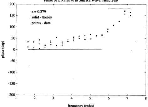
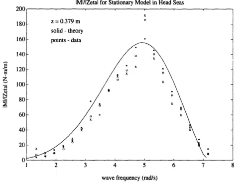
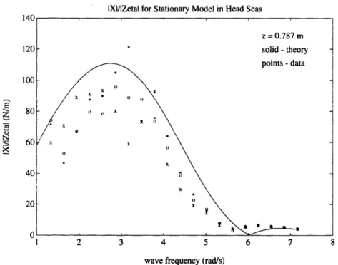
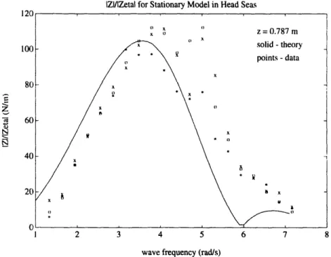
3.3.3.1 Stationary Model in Head Seas
Figures 3.6 through 3.8 compare theoretical and experimental transfer function
magnitude and phase information for X, Z, and M versus wave frequency for the model at a
centerline depth of 0.379 m. The theoretical curves were developed using the methods described
in chapter 2 with the body contour of the model taken into account. Similarly, figures 3.9
through 3.11 compare the same transfer function magnitude and phase information for the model
at a centerline depth of 0.787 m.
Resonance in the wave tank across its width at wave frequencies of 3.3 and 5 rad/s
appear to cause erratic data near these frequencies during the course of testing, and the result is
seen in the data presented here.
While the shallow and deep model data presented for the X and M transfer functions is
well predicted by the theory both in phase and magnitude, the method used to predict the transfer
function for Z fails to include a force component which accounts for the resultant vertical force
when the water wavelength is the length of the model body. The predicted zero in X is observed
at or near this frequency, as both figures 3.6 and 3.9 show in the magnitude and phase plots The
phase of this unpredicted Z force is consistent with that which would be expected of vertical drag
proportional to wave velocity in the aft section of the model body. The inclusion of such a drag
component into the heave force model was investigated, and produced a far worse low frequency
fit to the data than that presented in figures 3.7a and 3.10a. Because model accuracy is deemed
more important at lower frequencies where the majority of wave spectral energy is expected, the
previously developed model for heave force will be used in subsequent discussion.
It is seen that X, M and Z are all approximately linearly related to the wave amplitude
IXI/IZetal for Stationary Model in Head Seas
Z x X
2 3 4 5 6 7 8
wave frequency (rad/s)
Figure 3.6a Surge Force Transfer Function Magnitude for Shallow Model in Head Seas Note: The data points 'x', 'o', and '*' represent data taken from
the model under waves of increasingly higher amplitudes, respectively.
Phase of X Relative to Surface Wave, Head Seas
150 100 50 (0 -50 10( -150 2 3 4 5 6 7 8 frequency (rad/s)
Figure 3.6b Surge Force Transfer Function Phase for Shallow Model in Head Seas z = 0.379 solid - theory x points - data . X 0 } ,o ,, · . . : . I x x oI X I 0) - in) l~ · Ala.\ 2.-I _T1 . 1