Biologically inspired underwater propulsion and adhesion mechanisms

(1)

Biologically Inspired Underwater

Propulsion and Adhesion Mechanisms

MASSACHUSETTS MMMl.U.

by

OF TECHNOLOGY

OCT 16

2014

Yichao Pan

LIBRARIES

B.S., University of Notre Dame (2012)

Submitted to the Department of Mechanical Engineering in Partial Fulfillment of the Requirements for the Degree of

Master of Science in Mechanical Engineering at the

MASSACHUSETTS INSTITUTE OF TECHNOLOGY

September 2014

Signature redacted.

Signature of Author ...

Departnint of Mechanical eering Au st 8

Certified by

...

Si

gnature

redacted

7

~

angbae Kim

Assistant Profoorof Mec cal Engineering lehesis Supervisor

Signature redacted'

Accepted by ...

S...

David E. Hardt Chairman, Department Committee on Graduate Theses

(2)

(3)

Biologically Inspired Underwater

Propulsion and Adhesion Mechanisms

by

Yichao Pan

Submitted to the Department of Mechanical Engineering

on August 8, 2014, in Partial Fulfillment of the Requirements for the Degree of Master of Science in Mechanical Engineering

Abstract

The ultimate objective of this research is to develop an innovative underwater pipe inspection robot with both swimming and crawling capabilities as opposed to conventional in-pipe robots with wheeled designs or driven by propellers. The contents of this thesis include two different parts: a propulsion mechanism using a passive compliant tail and a reversible underwater adhesion mechanism.

The propulsion mechanism is the primary concern of this research. The hypothesis of this part of research is that a continuous passive compliant tail structure with an optimized stiffness profile in its longitudinal direction along with the proper control of a single actuator can allow the undulatory motion of this mechanism to resemble real fish swimming locomotion. This approach is in contrast to conventional approaches where multiple joints are actuated to create traveling waves to emulate propulsion mechanisms of fish. Four iterations of experiments are developed in total to verify the hypothesis, take measurements and improve the performance ofthe propulsion mechanism. It is proven that a continuous passive compliant structure driven by a DC motor through a four bar linkage can generate sufficient propulsion to drive a moving unit forward along a guide rail. The experiments with a simple prototype demonstrate that the propulsion mechanism is promising to drive a robot forward along a prescribed path without a guide rail. It is demonstrated that the stiffness profile in the longitudinal direction is one of the critical factors that affects the performance of the propulsion mechanism. A simulation model is developed to guide the design process of the passive compliant structure, mainly to optimize its stiffness profile along the tail structure. Special measures are implemented into the experiments to extract data to compare with simulated results.

The reversible underwater adhesion mechanism is another critical component of the underwater pipe inspection robot that is under development. The goal of developing a reversible underwater adhesion mechanism is to provide adequate traction to various surfaces while the robot operates in water. This reversible underwater adhesion mechanism allows a robot to stick and crawl in water pipes even across the stream. This mechanism may enable recharging capability extracting energy from kinetic energy of the pipe flow.

Two generations of robot prototypes are developed to demonstrate the crawling and propulsion mechanisms.

Thesis Supervisor: Sangbae Kim

(4)

(5)

Acknowledgments

First of all, I would like to express my gratitude to my supervisor, Dr. Sangbae Kim, whose expertise, understanding, and patience, added considerably to my graduate experience. He guided me through this research with his vast knowledge and skills in the field of robotics and mechanical design. I greatly appreciate the opportunity that he offered me to join his research group to learn more about robotics, which is a fascinating topic that I will keep following in my life.

I would like to thank Dr. Sami Habib at Kuwait University, who initiated this research and

collaborated with our group diligently. I sincerely appreciate the generous support from the Kuwait-MIT Center for Natural Resources and the Environment, where the research funding came from.

I would like to thank all my fellow labmates in the MIT Biomimetic Robotics Lab: Albert Wang, Michael Chuah, Matt Haberland, Haewon Park, Sangin Park, Joao Luiz Ramos and Will Bosworth. I would not be able to finish my research without their consistent support and valuable suggestions.

I would especially like to thank Dr. Franz Hover, who generously allowed me to set up the experiments in the testing pool in his lab. I also appreciate the help I received from Eric Gilbertson while doing experiments there.

My sincere thanks also go to Dr. Peko Hosoi, who provided great support to this research

project. I would like to thank Dr. Lisa Burton and Josh Wiens for sharing their abundant knowledge in fish swimming with me.

Last but not the least, I would like to thank my parents Fang Pan and Dongfang Shi for their tremendous support throughout my life. I would also like to thank my grandparents Zhihui Pan and Jingxian Bai, who raised me up and made me who I am today.

(6)

(7)

CHAPTER1

INTRODUCTION

The ultimate objective of this research is to develop an innovative underwater pipe inspection robot with both swimming and crawling capabilities as opposed to conventional in-pipe robots with wheeled designs or driven by propellers. The contents of this thesis include two different parts: a propulsion mechanism using a passive compliant tail and a reversible underwater adhesion mechanism.

The objective of the first part of this research is to investigate the application of a passive compliant underwater propulsion mechanism in the design of a fast swimming robot with high energy efficiency. This mechanism consists of one electric motor which enables undulatory motion of a slender and flexible structure with an optimized stiffness profile in the longitudinal direction similar to the body of an eel or lamprey.

Roboticists have been studying the compliance of legged robots, but so far there has been rarely any research on the role of compliance in swimming robots. Fish locomotion has been a long-lasting active research topic ever since 1930s. Biologists, mathematicians and roboticists have observed, investigated and categorized different modes of fish locomotion and developed a variety of theories and models to describe them. The diversity in body motions and anatomies and the complexity of hydrodynamic interactions prevent researchers from generating a simple and precise model to describe fish locomotion. A common approach taken by roboticists is to prescribe a kinematic configuration for a fish robot to follow by applying suitable control techniques to the actuators [1][2][3]. The kinematic equation is usually derived based on the observation of real fish and has a limited number of tunable parameters. Such fish robots generally have multiple discrete segments and actuators, thus having a restricted number of degrees of freedom. The dynamic interaction of the undulatory body with the surrounding water is too complex to model and often ignored in this kinematic approach.

In this research, a continuous passive compliant mechanism is adopted to replace the common mechanism with discrete segments. With only one actuator, the energy efficiency is expected to be superior to that of existing swimming robots with multiple actuators. An optimized stiffness profile in the longitudinal direction along with the proper control of the single actuator

(10)

allows the undulatory motion of this mechanism to resemble real fish swimming locomotion. The mechanism is back drivable due to its compliance, hence adapting to the surrounding liquid more easily. The robot is designed to swim fast while maintaining high energy efficiency.

A MATLAB simulation of the mechanism is generated based on the Lagrangian approach.

The typical hydrodynamic forces, such as drag and added-mass forces, are taken into account in the model, which can be used to obtain desired local material properties, in particular, stiffness. The aim of this simulation is to provide general insights to guide the design process of a swimming robot. Meanwhile, a series of experiments are conducted to verify the simulated results until an acceptable solution is found based on the design criteria.

Ideally, the intended mechanism should be modeled continuous, though it is considerably challenging to achieve this. It is worth to emphasize that our goal is not to build a highly precise model but rather to learn some general insights about this type of underwater flexible mechanism, especially its interaction with surrounding water. Therefore, the mechanism is modeled as a series of 2D rigid segments connected by pin joints with tunable stiffness. By increasing the number of segments and decreasing their lengths, this model can approach the continuous model. The stiffness of each joint can be optimized to achieve the maximum steady-state velocity of this mechanism. A prototype can thus be constructed based on this optimized stiffness profile.

Several iterations of experiments have been developed to verify the hypothesis and generate more insights to guide the design process. The passive compliant structure is molded with polyurethane with suitable elasticity. A DC motor is selected as the single actuator, and its continuous rotation is translated to oscillation through a four bar linkage. The propulsion mechanism is tested along a guide rail under water. A quick experiment off the guide rail proves that such a propulsion mechanism is promising to drive a robot forward along a prescribed path.

The objective of the second part of this research is to develop a reversible underwater adhesion mechanism. The pipe inspection robots developed recently use a range of different locomotion strategies, among which a combination of wheels and legs is the most common method. In-pipe wheeled robots apply a normal force against the pipe walls to maintain traction and gain propulsion by rotating the wheels [4]. The wheels are typically connected to and controlled by legs in a linkage mechanism with springs that generates a constant normal force, thus resulting in constant friction provided that the interior pipe diameter and surface roughness remains the same.

(11)

force to avoid unnecessary high friction and reduce the energy loss [5]. Most in-pipe wheeled robots adapt a design that includes three pairs of wheels 120 degrees apart in the cross-section view to support the robot body at the center of the pipe [6][7][8][9].

Most wheeled robots can only fit in a specified pipe size [6][7], while few models can operate within a limited range of varied pipe diameters [8]. The lack of adaptability to different pipe diameters and large cross-sections relative to the pipe interior greatly restrict the operation range of in-pipe wheeled robots. Another imposing challenge for in-pipe robots is power supply.

A number of robots are self-contained with embedded batteries [6], but many other wheeled robots,

including commercial models [9][10], are commonly tethered to external power supplies outside the pipe, which allows extended working hours and more embedded electric devices while restricting the operation range by the tether length [7][8]. Nevertheless, in-pipe wheeled robots generally can maintain sufficient traction and some existing models have the ability to maneuver through up to 90-degree turns, climb up a slope, or even crawl up vertically.

To overcome the limitations of wheeled design, a reversible underwater adhesion mechanism is designed to generate tractions for underwater robots. A micro active suction cup array (MASCA) actuated by a liquid pump is developed to demonstrate its feasibility of accomplishing reversible underwater adhesion.

Two generations of robot prototypes have been developed to demonstrate the crawling and propulsion mechanisms.

(12)

CHAPTER 2 SIMULATION OF PROPULSION MECHANISM

In order to guide the design of the propulsion system, a reasonably accurate simulation is desirable. Ideally the simulation is expected to predict an optimized stiffness profile that enables the design of a fast propulsion system while achieving high efficiency. In practice, simulation can never predict reality precisely. Therefore, the simulation is expected to show at least a general relationship between the stiffness profile and the corresponding swimming speed at different energy input levels. The error should be reduced as much as possible to improve the quality of the simulation. In this section, the theory that the simulation is based upon, the MATLAB scripts that have been used, and the preliminary results are discussed in detail.

2.1 LAGRANGIAN FORMULATION

In order to simulate the passive compliant underwater propulsion system, the first question that should be considered is how to model it. In reality the system is continuous with various stiffness along the longitudinal direction. To avoid using complicated differential equations to describe this system, the whole system is discretized into multiple rigid links connected by pin joints with adjustable stiffness. One of these joints is driven by an actuator. By increasing the number of links 'and decreasing their lengths, the multi-link model approaches to a continuous one. Furthermore, the model is assumed to be two dimensional. Thus, the problem has been simplified considerably to how to simulate a 2D multi-link rigid body system, which is a common type of mechanism to model.

The second question is how to obtain the equations of motion of such a system. The dynamic behavior is described in terms of the time rate of change of the mechanism configuration in relation to the joint torques exerted by the actuators. This relationship can be described by the equations of motion that govern the dynamic response of the links to input joint torques.

In general, two methods can be used to obtain the equations of motion: the Newton-Euler formulation, and the Lagrangian formulation. The Newton-Euler formulation is derived by the direct interpretation of Newton's Second Law of Motion, which describes dynamic systems in terms of force and momentum. The equations incorporate all the forces and moments acting on the

(13)

individual links, including the coupling forces and moments between the links. The equations obtained from the Newton-Euler method include the constraint forces acting between adjacent links. Thus, additional arithmetic operations are required to eliminate these terms and obtain explicit relations between the joint torques and the resultant motion in terms ofjoint displacements. In the Lagrangian formulation, on the other hand, the system's dynamic behavior is described in terms of work and energy using generalized coordinates. Therefore, all the workless forces and constraint forces and constraint forces are automatically eliminated in this method. The resultant equations are generally compact and provide a closed-form expression in terms ofjoint torques and joint displacements. Furthermore, the derivation is simpler and more systematic than in the Newton-Euler method [11].

When the system contains a small number of links, it is possible to use either formulation to derive the equations of motion. However, when the number of links increases, the Newton-Euler formulation requires tremendously more work than the Lagrangian formulation. In other words, the Lagrangian formulation is more scalable. Since the dynamic response of the system is the primary concern instead of the constraint forces, the Lagrangian formulation is feasible to solve the problem.

In the Lagrangian formulation, the mth (m = 1, ... , n) equation of motion is given by

daCL aIL 7- = C M ,M (2-1)

where L is the Lagrangian, which equals T- V. T is the kinetic energy, and Vis the potential energy.

q. is the mh generalized coordinate, and Qm is the m* generalized force.

2.2 ALGORITHM

Dr. Matthew Haberland in the MIT Biomimetic Robotics Lab developed a set of algorithms in

MATLAB to derive the equations of motion sysemticallyusing the Lagrangian formulation. The

set of algorithms has been modified extensively to serve the purpose of this project.

(14)

- The tail structure is simulated as a 2D model for simplicity. The entire structure has infinite

depth perpendicular to the 2D surface where the model is in. The thickness of each link is neglected, so the links are only varied by length.

- The continuous tail structure is approximated by a number of discrete rigid links, which

are connected by joints with tunable stiffness. Increasing the number of links can improve the accuracy of the model, but it also makes the simulation more computationally demanding.

- The hydrodynamic forces that are considered in the simulation include only the friction

and form drags and the added-mass forces. The friction drag acts parallel along each link, whereas the form drag acts perpendicular to each link. The expressions of the added-mass

forces are derived based on a 2D narrow rectangular model.

- The hydrodynamic forces are applied to the individual links separately. In reality the

hydrodynamic forces may be altered by interactions between the links, but this effect is neglected in the simulation. The links are almost independent to each other with interactions at the joints only. Turbulence is not considered in the simulation either because it is challenging to model in a simple way.

The set of algorithms contain two primary MATLAB files. The first file, deriveEoM.m, is used to derive the equations of motion symbolically. A set of MATLAB functions is generated automatically after running this file. The second file, simulate.m, is used to solve the equations of motion with numeric values of the variables involved in the equations. This file also calls a function, animation.m, to visualize the simulation in the form of an animation.

The equations of motion are derived by deriveEoM.m. Appendix A contains the MATLAB script.

The two variables, dim and pts, are defined at the very beginning of this file: dim defines

the number of links in the simulation, and pts defines the number of sample points along each link. The hydrodynamic forces acting on the links are calculated only at these particular sample points. These two variables make the simulation scalable. Ideally, both variables should be as large as possible in order to approach a real continuous system, but the computation becomes increasingly challenging if these two variables are large.

(15)

The number of degrees of freedom is determined by the variable dim. Besides the joint angles, there are two additional degrees of freedom, x and y, which indicate the horizontal and vertical positions of the origin of the first link, respectively. The linear and angular velocities and accelerations are defined.

A set of parameters that govern the geometric and inertial properties of each link are

defined, for example, the center of mass, length, moment of inertia, and neutral position. The stiffness of each joint, density of water, drag coefficients and torque input are defined as well.

The generalized coordinates q, velocities dq, and accelerations ddq are defined based on x,

y, and the joint angles.

A set of fundamental vectors are defined: ihat,jhat and khat, which determine the x, y and

z directions with respect to the fixed coordinate system. The vector er contains the directions along

each link, and the vector ern contains the directions perpendicular to each link.

The beginning and end points of the links are defined as pos. The midpoint of each link is defined as posM. The positions of sample points along each link is defined as posX. The velocities and accelerations corresponding to these points are defined subsequently.

The kinetic and potential energies of each link are defined as T and Ve, respectively. The power of each link is defined as P.

The hydrodynamic forces acting on each link are mainly the friction drag parallel to the link, defined as Fx, and the form drag and added-mass forces perpendicular to each link, together defined as Fy.

The generalized forces are defined as Qtau and QF, where Qtau is due to external torques and QF is due to external forces. For this project, Qtau is only due to the torque input at one selected joint.

R contains the key points that are used to generate the animation. It also defines the relative

sequence of these points.

There are three anonymous functions defined in this algorithm: ddt, F2Q and M2Q. ddt is a function for taking time derivatives. F2Q and M2Q calculate the force and moment contributions to the generalized forces.

After all the variable are initiated, the variables are represented in terms of the parameters and generalized coordinates using a loop. The hydrodynamic forces are generated using a function

(16)

HydroForce.m, presented in Appendix B. The friction drag that is parallel to each link is calculated

by

Fx= -PCd2VIVxl, (2-2)

where p is the density of water, Cd2 _{is the drag coefficient in the direction parallel to the link, and}

vx is the velocity of water parallel to the link. The sum of form drag and added-mass force that are

perpendicular to each link is calculated by

Fy= - PCd1VyJvy - lpmlay, (2-3)

where Cdl _{is the drag coefficient in the direction perpendicular to the link, vy is the velocity of} water perpendicular to the link, and ay is the acceleration of water perpendicular to the link.

After the variables are defined symbolically, the equations of motion are generated. This file generates a number of functions for simulate.m to call.

The simulate.m file, presented in Appendix C, contains the numeric values of the parameters defined in deriveEoM.m. These values can be easily adjusted in order to change the configuration of the mechanism.

After the parameters are given certain numeric values, the file uses ode45 to solve the equations of motion with the defined torque input. The equations of motion are called in the function dynamics.m, presented in Appendix D, which also contains the definition of the torque input.

The solution is input into animate.m function to generate the animation of the simulation.

2.3 PRELIMINARY RESULT

A few simulations with various parameters and number of links have been generated using this set of algorithms. Figure 1-1 shows the screenshots from the animation of one of the simulations. In this case the first link is twice as long as the following links. The actuator is located at the joint between the first and second links, where the torque is applied. The mass of the first link is larger compared to those of the following links.

(17)

The simulations verify the idea that such a mechanism driven by one actuator is able to propel itself forward in water. The remaining questions is, how to optimize the stiffness profile in the longitudinal direction.

Unit: m

(18)

2.4 DISCUSSION AND NEXT STEPS

It took a long time to set up the algorithms in a reasonable way. The major trouble that was encountered is how to calculate the hydrodynamic forces along the links. Ideally, the hydrodynamic forces should be integrated along each link. However, the direction of the force needs to be determined, which requires the use of either an abs or sign function in the integral. Somehow it is exceedingly difficult to find a way to integrate the hydrodynamic forces correctly to yield a reasonable simulation. Thus, an alternative way that is not as accurate as integration has to be adopted.

The idea is to discretize the hydrodynamic forces along each link and estimate the forces at a number of selected points. That is why a variable pts is defined in the derive EoM.m file. At each point, the direction and magnitude of the forces can be determined easily, so it is less computationally demanding compared to the integration method.

However, since the forces are expressed symbolically in the deriveEoM.m file, an increasing number of sample points makes the computation significantly more challenging. Also, an increasing number of links cause the same negative effect to the simulation as well. It is critical to find a method to simplify the computation such that it takes less time to derive the equation of motion. An intuitive method is to run the algorithm on a computer or server that has more computational power. Though MATLAB can convert files into C or other more fundamental computer languages in some cases to save the computing time, the symbolic toolbox has no such support at this point. A few unnecessary steps in the algorithm are taken out to cut down the computing time. For example, simplify function has a built-in loop to find the simplest expression of a symbolic term, which in general takes a long time to run. This function has very restricted uses in the algorithm.

Once the algorithm can generate equations of motion with a larger number of links and sample points, it is time to start working on the optimization algorithm. The goal is to attain an optimized stiffness profile along the longitudinal direction in order to maximize the steady-state forward speed given a certain torque input at one joint.

While working on the computer simulation, a series of prototypes are constructed to gain more insights experimentally.

(19)

CHAPTER 3 FIRST ITERATION OF EXPERIMENTS

After the simulation is constructed and started generating preliminary results, it is necessary to verify the results with experimental data. Experiments are also needed to tune the key parameters in the simulation, for example, the drag coefficients. More insights can be drawn from experiments to improve the design of the simulation. The primary objective of this research is to create a fast swimming robot with high energy efficiency. Therefore it is important to start designing the robot, at least the propulsion system, before the simulation can yield useful results.

3.1 PROOF OF CONCEPT

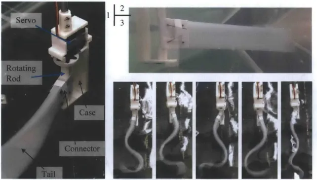
The overall hypothesis of this research is that a continuous passive compliant structure with an optimized stiffness profile in its longitudinal direction along with the proper control of a single actuator can allow the undulatory motion of this mechanism to resemble real fish swimming locomotion. The conventional approach of building a fish robot is to install a series of servo motors along the tail. Thus the tail would have multiple joints and discrete segments. The advantage of this approach is that the joint angles can be controlled precisely so that the overall shape of the tail at each time step will follow a desired trajectory, which is often extracted from experimental data based on extensive observations of real fish. However, it is not intuitive if a passive compliant structure driven by one single actuator is sufficient to generate propulsion to drive a robot forward. This is the fundamental layer of the overall hypothesis that needs to be verified. Once this part is verified by experiments, It can be investigated whether or not optimizing the stiffness profile would allow tbz propulsion mechanism to generate locomotion similar to real fish. Therefore, the first step of conducting the experipmnt Is to design a simple mechanism to prove that a passive compliant stnutie driv" btone 4jngle actuator is able to generate propulsion forward.

A preliminary experiment is performed to proveth* concept. The experiment set up is

illustrated in Figure 3-1 (1). The tail is made of E40flex@ upersoft 0030 (Smooth-on, Inc), which is flexible and neutrally buoyant in water. The taIl is-connected to a rod which rotates around the axis of the servo. The servo horn is inserted into the top section of the rotating rod to ensure firm connection between the servo and rod. The servo and rod are held together by the case. The servo

(20)

is controlled and powered by an Arduino Nano board, which is not shown in the figure. The case is connected to a six-axis force sensor by a metal rod along the servo's rotating axis. The force sensor is used to measure the propulsive force generated by the tail motion. LabVIEW DAQ (National Instruments Corporation) is used to acquire the experimental data. The servo is commanded to rotate back and forth periodically with respect to its neutral position. The amplitude is defined as the largest angle away from the neutral position in a view from the top. The frequency is controlled by how fast the servo changes the rotating direction. Both amplitude and frequency are variables in the experiment.

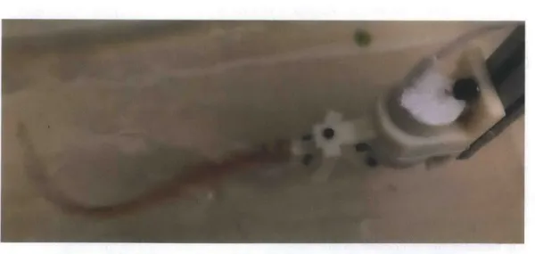
Figure 3-1 (2) shows the side view of the tail in a stable condition under water when it is not actuated. The material is neutrally buoyant in water. Though the tail is not able to support its own weight in air due to its outstanding flexibility, it nevertheless maintains its shape well under water due to buoyancy.

Several sets of experiment are performed by varying the amplitude and frequency. Figure

3-1 (3) contains a few pictures taken in real time when the tail is driven by the servo under water.

The tail is able to generate expected motions. The cross section of the tail tends to be thinner toward the end, so it seems floppy compared to the front part of the tail.

IKF

(21)

Figure 3-2 demonstrates the experimental results. Each color corresponds to a distinct value of amplitude. The delay time controls how fast the servo changes its rotating direction. For example, when the tail is rotated from the left end to the right end, it delays a certain number of seconds before being rotated back. The angle is measured with respect to the neutral position.

0.2 __1_1_1_1 o 22.5 deg 0 0.18 0 33.75 deg O 45 deg

8

o 56.25 deg 00.16 o 67.5 deg 20.14-a) 0.12 -ai) > 0 <0.1 - 0.08-0 0 .0 200 250 300 350 4 450

Delay (micro sec)

Figure 3-2. Proof-of-Concept Experimental Results (Thrust Measurement)

When the amplitude is relatively low (not greater than 45 degrees), the maximum thrust occurs at a moderate value of delay time (300 micro seconds). When the amplitude becomes larger (greater than 45 degrees), the thrust increases along with the increasing delay time. When the delay time remains constant, the thrust increases when the amplitude is greater. The only exception is when the amplitude equal to 67.5 degrees and the delay time equal to 200 micro seconds. In this case, the thrust is not the maximum compared to other data points with the same delay time. It is noticed that the servo does not reach the desired amplitude when the delay time is short (200 micro seconds). Further investigation is needed to understand this unexpected behavior of the servo.

The maximum thrust is 0.195 N, which occurs at the maximum value of both amplitude and delay time. This value seems small. It is suspected that the tail is too flexible to generate considerable propulsion. A stiffer tail may produce larger thrust. In addition, the desired motion

(22)

of the tail is unknown. The variables in this experiment are set based on intuition. More research should be done on the desired trajectory of the tail before generating commands for the servo. Nevertheless, the experiment assures that a servo can potentially drive the tail to follow a desired locomotion.

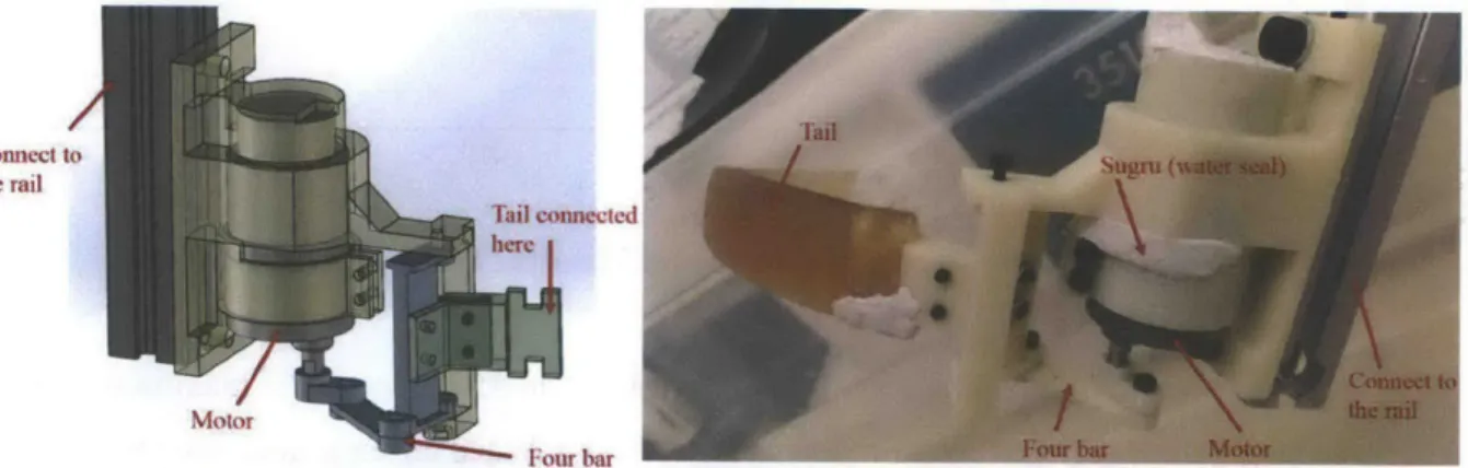
3.2 _{PRELIMINARY DESIGN}

The tail beating frequency is mostly constrained by the servo motor in the proof-of-concept experiment. It would be ideal to drive the tail with a conventional DC motor whose speed can be controlled easily by adjusting the voltage input. A preliminary design with a DC motor as the actuator is introduced in this section. To keep the experiment simple, the motion of the whole mechanism is constrained by a guide rail so that it can only move forward or backward along a straight line. Figure 3-3 illustrates the design ofthe mechanism as well as the prototype constructed based on the CAD model. The guide rail is not shown in the figure.

the rail

Tail connected

Motor

Four bar

Figure 3-3. The CAD Model and the Prototype of the Preliminary Design

B

rk kr a

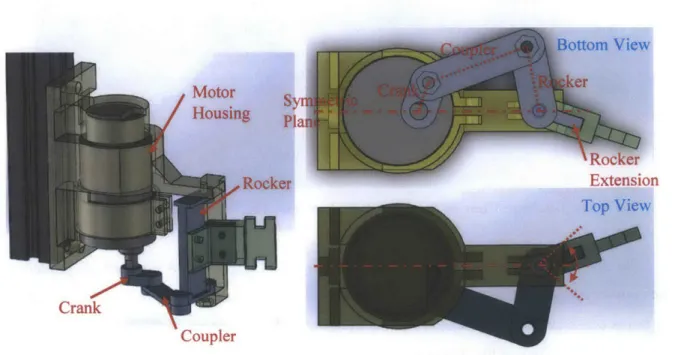
CrankRoe

(23)

Though it is intended to design a mechanism to verify the hypothesis quickly, it is not intuitive how to generate the undulatory motion in the soft tail made of rubber using a rotary motor. The key in this design is how to translate the rotation of motor into oscillation at the beginning of the tail with respect to an axis. In this design, a crank-rocker mechanism, one type of the four bar linkages, is adopted to achieve this function. Figure 3-4 illustrates a typical crank-rocker mechanism. A crank-rocker mechanism satisfies the condition that rl+r2 < r3+r4. The crank can

rotate 360 degrees continuously, while the rocker can only rotate through a limited range of angles. Typically a four bar linkage is planar, but in this design the crank-rocker mechanism is modified into a 3D version to accomplish the goal. The crank is directly connected to the shaft of the motor so that it can be driven continuously along with the motor shaft. The rocker is the purple piece that is connected to the green piece, which is a 3D printed plastic piece molded into the soft rubber tail. The purple piece that connects the crank and rocker functions as the coupler (r3 in Figure 3-4). The ground (ri in Figure 3-4) is integrated into the motor housing. In order for the beginning of the soft tail to oscillate symmetrically with respect to the symmetric plane of the motor, the rocker has an extension that forms an angle with the rocker. If the tail were connected to the rocker directly without this extension, the range of oscillation would not be symmetric with respect to the symmetric plane of the motor. Figure 3-5 illustrates the arrangements in different

views.

(24)

The dimensions of the crank-rocker mechanism are determined in a sketch in SolidWorks. The major factors that are taken into account include the dimensions of the motor and the molded tail, which is decided to be 24 cm long. Since the tail is expected to be molded with polyurethane or silicone rubber and the molds are 3D printed using the Stratasys@ Dimension printer readily available in the lab, the length of the tail is constrained by the maximum dimension of the molds that can be produced on the printer. The lengths of the rocker, coupler and crank are determined roughly based on the outer radius of the motor and the length of the tail. The range of oscillation of the extension of the rocker, which is connected directly with the beginning of the tail, is also determined based on a reasonable estimation. In short, the specific dimensions of the entire setup are not optimized with respect to any criteria to achieve high performance. Again, the goal is to set up a mechanism that can quickly verify the hypothesis that a passive compliant tail driven by one single actuator can generate propulsion that is sufficient to propel the whole system forward.

3.3 PROTOTYPE

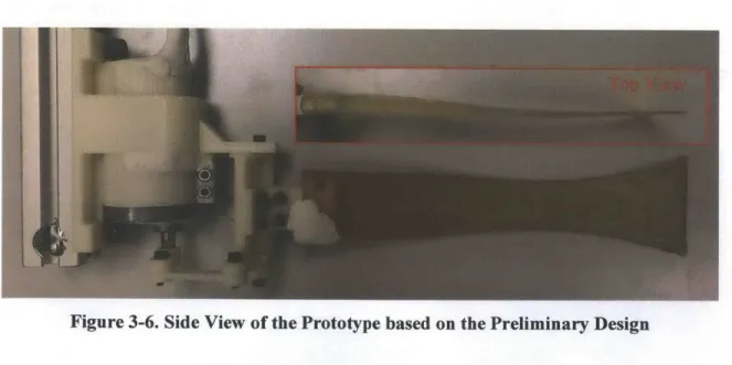
Figure 3-6 illustrates the side view of the prototype based on the preliminary design.

Figure 3-6. Side View of the Prototype based on the Preliminary Design

The shape of the tail is designed to be similar to that of a real fish. A piece of 3D printed plastic is overmolded into the tail so that it is easier to connect the tail with the rocker. The length of the tail is constrained by the capacity of the 3D printer. The thickness of the tail varies along with the length. It is thick at the beginning and becomes thinner toward the end. The width of the

(25)

tail also varies along with the length. It first gets narrower and then wider at the end. Since the material is homogeneous except the 3D printed piece at the beginning, the stiffness is largely correlated with the local geometry. The tail is rigid at the beginning, especially the section that contains the 3D printed part, but the end of the tail is floppier compared to the rest of the tail, although the area in the side view is larger. Similar to the design of the crank-rocker mechanism, the specific dimensions of the tail are determined based on estimation rather than rigorous analysis or simulation. Eventually the design will be guided by the simulation, but there is not enough information at this stage yet, nor is it necessary to bring in the simulation for this simple setup that is used to verify the hypothesis.

In addition to the geometry, the material that is used to mold the tail also affects the stiffness significantly. The tail can neither be too rigid nor too floppy in order to create a reasonable undulatory motion that is able to generate propulsion. Based on the experience dealing with the Smooth-On® materials, mainly the EcoFlex@ and VytaFlex® series, the VytaFlex® 20 is selected due to its relatively low viscosity and appropriate flexibility. The VytaFlex@ 20 consists of two liquid parts that are mixed together according to 1:1 volume or weight ratio. The viscosity while the mixed material is still liquid largely affects the quality of the final product, because it needs to be put in a vacuum chamber to degas, a critical process that reduces the number of air bubbles in the final product. If the viscosity ofthe mixed material in the liquid state is too high, the air bubbles would be trapped in the product and mold, and the final product after sufficient solidification would be undesirably porous. VytaFlex® 40 and 60 are stiffer and more difficult to degas than VytaFlex® 20. EcoFlex® 0010 and 0030 are too flexible and easy to deform. Therefore, VytaFlex® 20 is selected to make the tail in this prototype.

The motor used as the sole actuator in this design is the 19:1 Metal Gearmotor 37Dx52L mm with 64 CPR Encoder purchased from Pololu [13]. The major advantages of using this motor include: (1) it is inexpensive, (2) it comes with an encoder attached, and (3) it is expected to deliver sufficient power to drive the tail under water. The very first concern of this experimental setup is how to make the motor waterproof so that it can operate under water. That is why the motor housing covers around the motor to avoid direct exposure to the water. Sugru@ is a type of self-setting rubber that is used to enhance the waterproof capability of the setup. It is mainly applied to seal the gap between the motor and motor housing, as well as the holes on the external surface of the motor that is not covered by the motor housing. The only interface that is vulnerable to water

(26)

penetration is around the motor shaft. In order to ensure that the motor shaft can spin freely, no sugru or other sealant is applied around the shaft. The motor comes with lubrication between the shaft and the stationary part, and it is assumed that the lubrication is able to prevent water from flowing into the motor easily.

The motor is powered by an external power supply that is connected with the motor through a long wire. Ideally batteries should be carried on board in the final product. But to keep the setup simple to use without worrying about maintaining stable and sufficient power input into the system, a power supply with adjustable voltage output is adopted to power the motor. The power supply is kept away from water during the experiment to ensure safety.

The motor housing is bolted onto an aluminum extrusion which is attached to a carriage constrained on a linear guide rail. The carriage can move freely along the rail with low friction. The experiment is conducted in a plastic storage container that is roughly 50 cm long, 35 cm wide and 40 cm tall. The water level is about 20 cm above the bottom of the container, and the motor and tail assembly is entirely submerged under water. The guide rail is positioned right above the container and sits on its top edges. The motor is intended to operate at 12 V, but it can start rotate when the voltage is as low as 1 V. Since the motor operates under water, the problem of overheating is less of a concern. The voltage input ranges between 1 V up to 25 V during the experiment, and the motor speed does not seem to saturate yet. A video of the experiment is available on YouTube [14]. A screenshot of the video is shown in Figure 3-7. The guide rail is not present in the camera view.

(27)

Though no measurement is performed during this experiment, the objective of quickly verifying the hypothesis that a passive compliant tail driven by one single actuator can generate propulsion that is sufficient to propel the whole system forward is successfully attained. As shown in the video, the motor drives the tail through the crank-rocker mechanism and the tail oscillates around the axis within a range that is symmetric about the symmetric plane of the motor. More importantly, while the beginning of the tail is oscillated by the rocker, a clear undulatory motion is generated throughout the tail, which propels the whole unit forward along the guide rail with appreciable speed that is seemingly proportional to the voltage input applied to the motor. The response of the system is quick: when the power supply is turned on, the tail starts oscillating; when the voltage input gets higher, the frequency of tail oscillation increases at the same time, which results in a higher forward speed. It can be concluded that the hypothesis is correct and more rigorous experiments and analyses are worth to be carried out to further investigate how to improve the performance of the propulsion system. In particular, it needs to be investigated whether or not adjusting the stiffness of the passive compliant tail would improve the system performance to yield a fast swimming mechanism with high energy efficiency.

(28)

CHAPTER 4 SECOND ITERATION OF EXPERIMENTS

Based on the promising results from the preliminary experiment, an improved version of experiment is designed to gather useful data for further analysis and investigate the effects of some selected parameters on the performance of the system.

4.1 EXPERIMENTAL SETUP

In this iteration, the motor is kept the same to avoid major modifications in the design. Ideally a smaller motor can be used to reduce the total weight of the moving unit so that it may be easier to incorporate into the robot design in the future. But to save time and take advantage of the large quantity of such motors available in the lab, the same type of motor is used as the sole actuator to drive the tail. In addition, the material that is used to mold the tails also stays the same. The tails tested in this iteration have different dimensions, which are the main focus of the study at this stage. It would take much more time to test a variety of materials. The projected lengths of the crank, coupler and rocker in a 2D sketch similar to Figure 3-5 are not altered either.

Stainless

Steel

Shaft

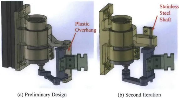
Plastic Overhang

(a) Preliminary Design (b) Second Iteration

(29)

The motor housing and the crank-rocker mechanism are slightly modified to enhance the stability of the system. The CAD model of the improved version is illustrated in Figure 4-1, along with the comparison with the preliminary design. The most important difference is that in the improved design the rocker is connected with the motor housing through a steel shaft that has significantly higher Young's modulus than ABS plastic, which is the common material used by

3D printers. The rocker rotates freely around this shaft, which is tight fit into the motor housing

and further secured with screws. In the preliminary design, the rocker is connected to the motor housing with an integrated overhang that is also 3D printed with ABS plastic. The superior Young's modulus of steel enhances the bending rigidity and thus reduces the undesired movement of the axis around which the rocker rotates.

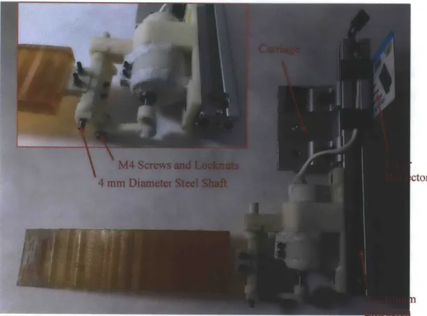
Some additional improvements in the second iteration include: (1) the crank, coupler and rocker are thicker than before, (2) the screws that connect the crank, coupler and rocker are changed to M4 Friction-Resistant Brass Shoulder Screws (McMaster-Carr@) Part No. 9845 1A 117), instead of M2.5 zinc-plated steel screws used in the preliminary design, and (3) the nuts are replaced with M4 316 Stainless Steel Nylon-Insert Hex Locknut (McMaster-Carr® Part No.

94205A230). The increased thickness of the components reduces undesired deformation while the

motor speed is high, though the components never experienced serious trouble during the preliminary experiment. A shoulder screw has a smooth surface that is not threaded. The components are specifically designed to take advantage of the shoulder area so that they can rotate around the smooth surfaces, which reduce friction during rotation. The locknuts can effectively prevent the screws from loosening during the experiment. Brass and 316 stainless steel are more resistant to water corrosion, so the screws and nuts are less likely to rust, which maintains the smoothness of the interface between the plastic components and screws. Figure 4-2 demonstrates the prototype based on the second iteration, and the carriage is also included in the figure. The total weight of the unit is 898.9 g.

The change in the experimental setup is that the guide rail is replaced by a 4 m long one that is available in the lab. The type of carriage and guide rail is Speed Demon OSG-25 purchased from LM76 [15]. The main reason to use such a long guide rail is toneasure how long it takes for the system to reach steady speed after the motor starts rotating while keeping the voltage input constant. The long distance allows adequate time for the system to reach steady state.

(30)

ctor

Figure 4-2. Prototype based on the Second Iteration of Design

e Sensor

(31)

It is challenging to set up such a long guide rail in an environment with water. Thanks to Prof. Franz Hover, the entire experimental setup could be installed in the giant testing pool in MIT

1-225 (Building 1 Room 225). The entire guide rail is supported by three aluminum extrusions

vertically, and it is suspended right above water to avoid total submergence and potential corrosion. The guide rail is not easy to be disassembled from the supporting structure for frequent maintenance. The carriage, connected with the motor and tail through a short aluminum extrusion, is put on and taken away from the guide rail before and after each experiment. The distance between the guide rail and water surface is adjusted carefully so that the tail can be entirely

submerged under water. Figure 4-3 (a) demonstrates the setup of the guide rail.

(a) Laser Distance Sensor (b) Current Sensor (c) Multifunction DAQ Figure 4-4. Sensors and DAQ

To measure the speed of the unit that is propelled by the oscillating tail, a Micro-Epsilon optoNCDT ILR 1030 Laser Distance Sensor, shown in Figure 4-4 (a), is installed at the end of the guide rail [16]. The measuring range of this type of sensor is between 2 m and 50 m, and more importantly, the response time is merely 10 ms. The short response time is critical because the distance that needs to be measured is constantly changing while the unit is moving along the guide rail. If the response time were too long, the distance measurement would not be accurate for further analysis to obtain speed measurement. A plastic card with reflecting tape on the side facing the laser sensor is attached to the aluminum extrusion that connects the carriage and motor housing. This card is intended to reflect the laser more effectively so that the laser sensor can measure the changing distance continuously. A mechanical stop is installed right in front of the laser sensor to

(32)

avoid collision and prevent the moving unit from falling from the guide rail when it reaches the

end.

To measure the power input into the system, an ACS714 Current Sensor Carrier from Polulu, shown in Figure 4-4 (b), is installed along the wire that connects the power supply and the motor [17]. This current sensor measures +/- 5 _{A current with a typical error of}_+/-_{1.5%. The}

voltage remains constant throughout each individual experiment, so the power input can be calculated by multiplying the measured current and the set voltage. It is essential to measure the power input in order to compute the cost of transport when analyzing the system performance.

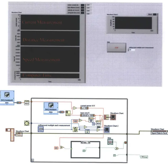
Wawform chart

Hiisi-171P

Figure 4-5. LabVIEW Program for Data Acquisition

I.

I

DAQANNUW

(33)

To record the distance measurement from the laser sensor and the current measurement from the current sensor simultaneously, it is necessary to set up a data acquisition system that displays the data in real time for quick verification and records the data in an organized and convenient way. A National Instruments@ USB-6009 Multifunction DAQ, shown in Figure 4-4 (c), is adopted to convert the analog inputs from the current and laser sensors into digital signals and transfer the data into a laptop that runs a customized LabVIEW program, which displays the data in real time and exports them into Excel spreadsheets. The DAQ has an analog-to-digital-conversion resolution of 14 bit and the maximum sampling rate of 48 thousand samples per second, which are more than enough for this application. Figure 4-5 demonstrates the LabVIEW program that was built with the help from Albert Wang, a Ph.D. candidate in the MIT Biomimetic Robotics Lab. The current and distance measurements are directly acquired from the DAQ. The speed measurement is the instantaneous differential of the distance measurement. It is mainly recorded for verification purpose during data analysis, but in fact the speed data are not used for analysis.

10V 1 CC

Gigur 4-6 Oser a lEnsor l GND

A10

+5 V _{N1 DAQ}

GND

10-20 V I in I out

JJGND0

(34)

A resistor needs to be connected between the ground and output pins of the laser sensor.

The resistance value must be calculated carefully. According to the manual of the laser sensor, the default setting of the analog output is 4 mAcorresponding to 200 mm, and 20 mA corresponding to 5000 mm. Since the total length of the guide rail is 4 m, it is not necessary to adjust the setting. The analog input pins on the DAQ can take up to 10 V, but the resistor value is calculated for Arduino Uno, whose analog input pins can only accept voltage input up to 5 V. To map the 4 -20 mA current output from the laser sensor into the 0 -5 V voltage input that is acceptable to Arduino

Uno, a 249-Ohm resistor is placed between the ground and output pin of the laser sensor. A 499-Ohm resistor can be used instead to fit better with the DAQ. But since the resistor is soldered onto the laser sensor already, it is not changed for this experiment.

To capture the motion of the tail while it is propelling the moving unit forward along the guide rail, a GoPro@ Hero3+ Black Edition camera is used to record videos during experiments

[18]. The GoPro® camera has a few advantages: (1) it comes with a waterproof housing, (2) it is

able to shoot videos at a high frame rate (up to 240 frames per second under WVGA mode), and

(3) it is inexpensive, versatile and shoots high quality videos. The camera is installed on a carriage

which slides along a guide rail into water, as shown in Figure 4-3 (c) and (d). The camera faces upward to capture the motion of the tail under water while it passes through the camera view. If the camera were placed above water, the reflection of light by the water surface might block the camera view and the camera would not be able to capture the tail motion clearly. An LED light is also installed right next to the camera to provide more lighting while the videos are taken.

The mechanism is designed in a way that the tail can be easily assemble and disassemble from the rocker. The tail and the rocker are connected with four M2.5 screws. The tail and rocker are not fabricated as one piece because a series of different tails are expected to be tested, and separating those two parts simplifies the process of swapping tails. In this iteration of experiments, four tails are fabricated, as shown in Figure 4-7. All the tails are molded with Vytaflex@ 20 regardless of the different colors shown in the figure. An engineer at Smooth-on® verified that the material properties should be the same even though the color of the material varies. The tails are different in two dimensions: width and initial thickness at the conjunction with the 3D printed connector. The thickness varies linearly along with the length. The initial thickness of each tail is indicated in Figure 4-7. The width stays constant along the length. All four tails are 19-cm long,

(35)

constrained by the maximum size of the tail molds that can be fabricated on the 3D printer available in the lab. The name of each tail is listed on the left in Figure 4-7.

3 cm wide

3 cm wide

5 cm wide

Figure 4-7. Four Types of Tails

4.2 RESULTS AND DISCUSSION

A series of experiments were conducted with three controlled variables: (1) width of the tail, (2)

thickness of the tail, and (3) voltage applied to the motor. There is a large number variables that can be chosen to vary during experiments, for example, material of the tail, length of the tail, type of the motor, range of oscillation of the tail, just to name a few. It is infeasible to vary so many different properties in a limited number of experiments. Therefore the study focuses on the

influence due to merely three variables on the system performance.

A video that was shot outside the testing pool is available on YouTube [19]. A screenshot

of the video is shown in Figure 4-8. It demonstrates how the tail propels the whole unit forward along with the guide rail. Another video that was shot using the GoPro@ camera under water is also available on YouTube [20]. This video demonstrates the undulatory motion of the tail under water while it is moving forward. It is noticed that the tail may be too close to the water surface such that while the system is operating, the tail generates appreciable but undesirable splashes which increase the drag that the system needs to overcome. Figure 4-9 presents the current vs. time and distance vs. time plots for the experiment on the Thick Narrow tail when the voltage input is 20 V. In the distance vs. time plot, the distance measurements are reversed. At the beginning of

(36)

each experiment, the measured distance should be the largest, while the moving unit is far away from the laser sensor. The measured distance should be decreasing while the moving unit is moving toward the laser sensor positioned at the end of the guide rail. The LabVIEW data acquisition system is turned on before the motor is activated in each experiment, so the laser sensor measures the constant distance and the current sensor measures zero current for a few seconds while the moving unit is stationary at the beginning.

Figure 4-8. A Screenshot of the Experiment Video

Current vs. Time 20V Thick Narrow 2

6 5 --4 3 S(a) 1U 1. 6 10 12 Time [s]

Figure 4-9. Current vs. Time

Distance vs. Time 20V Thick Narrow 2 :tr (a) 3 2.5 2 1.5 0.5 (b) _0 2 4 6 a Time []

and Distance vs. Time (b) Plots

12

10 1

(37)

Each tail is tested at five different voltages (5 V, 10 V, 15 V, 20 V and 25 V), so there are 20 individual experiments in total. In the current vs. time plot, the current value is around zero before the power supply is turned on to apply a voltage on the motor. The current value shoots up when the power supply is switched on, and it oscillates roughly around a constant value while the moving unit is propelled forward by the tail along the guide rail. The current does not stay constant because the amount of reaction force exerted by the crank-rocker mechanism and the connected tail that the motor needs to overcome is varying during operation. Instead of using instantaneous values to represent current during each experiment, the average value of the instantaneous values after the transient phase is used. For example, the average value of current after 2 s in Figure 4-9 (a) is about 1.7 A. Eliminating the transient phase, the distance vs. time curve is close to a straight line with a constant slope. The average speed of the moving unit in each experiment can be estimated as the slope of this straight line. For example, in Figure 4-9 (b), the slope of the straight line before 10 s is about 0.33 m/s, which is regarded as the average speed of the moving unit. A MATLAB script, presented in Appendix E, is written to process the current and distance data for all 20 experiments together and generate summary plots to compare the experiments.

Figure 4-10 illustrates the average speed vs. average current plot and Figure 4-11 illustrates the cost of transport vs. voltage for all 20 experiments. There are four curves with distinct colors, each representing a type of tail. Table 4-1 summarizes the data based on the different types of tails. As shown in Figure 4-10, a general trend is that for each tail, as the voltage input increases, the average current and the average speed both increase with diminishing margin. The average speed starts to saturate after the voltage input exceeds 15 V, even though the current drawn keeps increasing. Overall the Thin Wide tail, shown in pink, seems to have the best performance among all four tails, as its average speed at each different voltage level is better than that of any other three tails. The Thin Wide tail also achieves the highest speed, which is 0.43 m/s when the voltage input is 25 V. The Thick Wide, Thick Narrow and Thin Narrow are ranked the second, third and fourth places, respectively, according to the average speed at each voltage level. The order is consistent with respect to voltage, as shown more clearly according to the data summarized in Table 4-1.

(38)

I I I I I I I I I

--- Mick VWh_, 25V Thin Wide

0.4 - - Tbick Name 20V V Tin Wde

25V Thick Wide

0.35 - M

Te Nuawn V Thck Wde 25V Thick Narrow

-ck Narrow -25V Thin Narrow 03 ThnVTinNro 0.25 - 10V Thick Wide-0.2-10V 'ck Narrow 0.15 - 10V nN o 0.1 -Thin de 0.06 -5V Th V Thick Wide 5V Thick Narrow I I I I I I I I I-W4 0.6 0.8 1 1.2 1.4 1.6 1.8 2 2.2 2.4

Average Current [A]

Figure 4-10. Plot of Average Current vs. Average Speed

It is not fair to compare the performance of the system with different tails based on the average speed only, because apparently the current drawn during each experiment varies as well. Therefore the cost of transport is brought in as a critical criterion to evaluate the system performance. The cost of transport quantifies the energy efficiency transporting an animal or vehicle from one place to another. It is defined according to Eq. (4-1) below:

COT = , (4-1)

Mgv

where COT represents the cost of transport, P is the power input to the system, m is the mass of the system, g is the gravitational acceleration, and v is the constant velocity of the system [21]. The power input to the system is calculated as the product of the average current and set voltage for each experiment.

(39)

Table 4-1. Summary of Data for Different Tail Types Voltage [V] 5 10 15 20 25 Current [A] 0.56 0.99 1.34 1.70 2.18 Thick Narrow Speed [m/s] 0.04 0.21 0.32 0.33 0.36 CoT 8.97 5.55 7.28 11.79 17.28 Voltage [V] 5 10 15 20 25

Thick Wide Current [A] 0.68 1.18 1.49 1.73 1.76 Speed [m/s] 0.05 0.25 0.36 0.39 0.39

CoT 7.86 5.40 7.20 10.12 13.04

Voltage [V] 5 10 15 20 25

Thin Narrow Current [A] 0.49 0.80 1.08 1.36 1.57 Speed [m/s] 0.04 0.16 0.26 0.28 0.31

CoT 7.35 5.86 7.11 11.31 14.50 Voltage [V] 5 10 15 20 25

Thin Wide Current [A] 0.60 1.04 1.49 2.05 2.14 Speed [m/s] 0.06 0.26 0.38 0.41 0.43

CoT 5.53 4.51 6.83 11.53 14.48

According to Figure 4-11, overall the lowest cost of transport occurs at 10 V when experimenting on the Thin Wide tail, which is 4.51. The Thin Wide tail also has the lowest cost of transport at 5 V, 10 V and 15 V, compared with the other tails. On the contrary, the Thick Narrow tail has the highest cost of transport at all voltages except at 10 V, where the Thin Narrow tail tops the other tails. Evaluating the data of cost of transport leads to a preliminary conclusion that tails with larger side area and smaller cross-sectional area tend to have lower cost of transport.

(40)

5 10 15

Voltage []

20 25

Figure 4-11. Cost of Transport vs. Voltage

The larger side area means the tail can push more water around while oscillating and thus

can generate higher propulsion if the frequency is roughly the same when compared to those with smaller side area. If a small segment of the tail, viewed from the top, is considered for analysis for example, the same driving frequency of the tail is equivalent to the same change in linear velocity relative to surrounding water. A tail with larger side area would have more segments like this that can accelerate more water simultaneously and thus the change in linear momentum would be larger than that produced by a tail with smaller side area. The angular speed of the motor is inevitably

18 16 - 141-12 U 10 8 6 4 25V Thick Narrow -- Tick Natrow - TlinmWie 25V Thi ide 25V Thi Narrow 25 Th Wide Thic arrow OV Wide 20V in Narrow 20V Thick Wide 5V Thick Narrow 5V ickWide l5arrow5Thick Narrow

I arrowV Thick Wide

15V Thin 5V Thin Narrow

in arrow

05V Thin Wide kNarrow

10 ick Wide 10V Thin Wide

Biologically inspired underwater propulsion and adhesion mechanisms

Biologically Inspired Underwater

Propulsion and Adhesion Mechanisms

by

OCT 16

2014

Yichao Pan

LIBRARIES

Signature redacted.

Certified by

...

Si

gnature

redacted

7

angbae Kim

Signature redacted'

Accepted by ...

S...

Biologically Inspired Underwater

Propulsion and Adhesion Mechanisms

by

Yichao Pan

Abstract

Acknowledgments

CONTENTS

CHAPTER1

INTRODUCTION

CHAPTER 2

SIMULATION OF PROPULSION MECHANISM

2.1

LAGRANGIAN FORMULATION

2.2

ALGORITHM

2.3

PRELIMINARY RESULT

2.4 DISCUSSION AND NEXT STEPS

CHAPTER 3

FIRST ITERATION OF EXPERIMENTS

3.1

PROOF OF CONCEPT

IKF

8

3.2

PRELIMINARY DESIGN

3.3

PROTOTYPE

CHAPTER 4

SECOND ITERATION OF EXPERIMENTS

4.1

EXPERIMENTAL SETUP

Hiisi-171P

I

3

cm wide

4.2

RESULTS AND DISCUSSION

_{PRELIMINARY DESIGN}