Publisher’s version / Version de l'éditeur:
International Journal of Intelligent Systems, 26, 5, pp. 444-463, 2011-06-01
READ THESE TERMS AND CONDITIONS CAREFULLY BEFORE USING THIS WEBSITE.
https://nrc-publications.canada.ca/eng/copyright
Vous avez des questions? Nous pouvons vous aider. Pour communiquer directement avec un auteur, consultez la Questions? Contact the NRC Publications Archive team at
[email protected]. If you wish to email the authors directly, please see the first page of the publication for their contact information.
NRC Publications Archive
Archives des publications du CNRC
This publication could be one of several versions: author’s original, accepted manuscript or the publisher’s version. / La version de cette publication peut être l’une des suivantes : la version prépublication de l’auteur, la version acceptée du manuscrit ou la version de l’éditeur.
Access and use of this website and the material on it are subject to the Terms and Conditions set forth at
Alternative Approach for Learning and Improving the MCDA Method
PROAFTN
Al-Obeidat, Feras; Belacel, Nabil
https://publications-cnrc.canada.ca/fra/droits
L’accès à ce site Web et l’utilisation de son contenu sont assujettis aux conditions présentées dans le site LISEZ CES CONDITIONS ATTENTIVEMENT AVANT D’UTILISER CE SITE WEB.
NRC Publications Record / Notice d'Archives des publications de CNRC: https://nrc-publications.canada.ca/eng/view/object/?id=177a0a74-8642-4b1e-a695-9a0a8643ba8e https://publications-cnrc.canada.ca/fra/voir/objet/?id=177a0a74-8642-4b1e-a695-9a0a8643ba8e
Alternative Approach for Learning and
Improving the MCDA Method PROAFTN
Feras Al-Obeidat
Department of Computer Science University of New Brunswick
100 Tucker Park RD,Saint John, NB,E2L 4L5, Canada [email protected]
Nabil Belacel
NRC Institute for Information Technology
Suite 1100 Scientific Park, Moncton, NB E1A 7R1, Canada [email protected]
December 11, 2009
Abstract
OBJECTIVES. The objectives of this paper are 1) to propose new techniques to learn and improve the multi-criteria decision analysis (MCDA) method PROAFTN based on machine learning approaches, and 2) to compare the performance of the developed methods with other well-known machine learning classification algorithms. METH-ODS. The proposed learning methods consist of two stages: the first stage involves using the discretization techniques to obtain the re-quired parameters for the PROAFTN method, and the second stage is the development of a new inductive approach to construct PROAFTN prototypes for classification. RESULTS. The comparative study is based on the generated classification accuracy of the algorithms on the datasets. For further robust analysis of the experiments, we used the Friedman statistical measure with the corresponding post-hoc tests. CONCLUSION. The proposed approaches significantly improved the performance of the classification method PROAFTN. Based on the generated results on the same datasets, PROAFTN
outperforms widely used classification algorithms. Furthermore, the method is simple, no preprocessing is required, and no loss of infor-mation during learning.
Keywords: Knowledge Discovery, MCDA, PROAFTN, Discretization,
In-ductive Learning.
1
Introduction
There are huge amounts of data being collected in databases every day. As a result, a massive amount of information is located in these databases; the knowledge within them is most likely important, but has yet to be identified or expressed. Since discovering this hidden knowledge goes beyond human ability to analyze and discover, the use of automatic techniques to retrieve this knowledge will help. It is necessary to use advanced tools to simplify and automate the process of extracting this kind of information from large stores of data and representing it in a useful form. Machine learning is a significant approach for gaining new and valuable knowledge [47, 37]. It does so by analyzing the information that resides in data using advanced algorithms and modeling techniques. This knowledge, for instance, enables a decision maker (DM) to identify market trends, or can assist in disease diagnoses, and can ultimately support and facilitate the making of well-informed decisions [1, 29, 45].
This paper is mainly concerned with the supervised learning approach where the given instances have known class labels, and the target is to build a model from this data to classify other unclassified data. We will focus on the classification problems in which the output of instances admits only discrete or nominal values describing the number of classes residing in the dataset [17, 33].
Classification problems require the development of a classification model that identifies the behaviors and characteristics of the available objects to rec-ommend the assignment of the new undefined objects to predefined classes [29, 44]. The significance of classification problems has motivated the de-velopment of a number of techniques for constructing classification models. Statistical techniques [47, 48] have been playing a pioneering role in classifi-cation paradigms for many years, but recently other approaches have become popular, mainly from the fields of machine learning, operation research, and Multiple Criteria Decision Analysis (MCDA) [43, 50].
In MCDA the classification problems can be distinguished from other classification problems within the machine learning framework from two per-spectives. The first includes the nature of the characteristics describing the objects, which are assumed to have the form of decision criteria providing not only a description of the objects but also some additional preferential information associated with each attribute [36, 51]. The second includes the nature of the classification pattern, which is defined in both ordinal and nominal terms [5, 19, 34]. Classification models developed through machine learning techniques usually fail to tackle these issues, focusing basically on the accuracy of the results obtained from the classification model [51]. However, the main problem associated with MCDA is that the classification models do not automatically result only from the vectors describing the objects, but depend also on the judgment of a DM. The DM defines the boundaries of the attributes and the weights which define the importance of each attribute in the dataset [19, 21]. However, it is usually difficult for a DM to assign accurate quantitative values to these parameters. Moreover, the parameters which represent the preferences are often unclear and may change with time. For these reasons, it is rational to avoid questioning the DM for accurate parameter values. As an alternative approach, the utilization of machine learning techniques to infer these parameters from the dataset is more ap-propriate. This is the general focus of this paper. In the problem statement, more discussion will be carried out.
The problem of assigning objects to predefined classes in (MCDA) is known as a “multiple criteria sorting problem” [43, 52]. This consists of the formulation of the decision problem in terms of the assignment of each object to one or several classes. The assignment is achieved through the ex-amination of the intrinsic value of the objects by referring to pre-established norms, which correspond to vectors of scores on particular criteria or at-tributes, called profiles [8, 36]. These profiles can separate the classes or play the role of central reference points in the classes. Therefore, following the structure of the classes two situations can be distinguished: ordinal and nom-inal sorting problems. The cases where the classes are ordered are known as “ordinal sorting problems” and are characterized by a sequence of boundary reference objects. Scoring of credits is an example that can be treated using this problematic. The cases where the classes are not ordered are known as “nominal sorting problems”, also called “multiple criteria classification problems” (MCCP), and are characterized by one or multiple prototypes. Each prototype is described by a set of attributes and is considered to be
a good representative of its class [31, 51]. This paper will focus on a new multiple criteria classification method PROAFTN [6] that has been recently developed. To apply PROAFTN, we need to determine the values of several parameters prior to classification, such as boundaries of intervals, weights and thresholds. This consists of the formulation of the decision problem in terms of the assignment of each object to one or a number of classes.
Some techniques have previously been used to determine these intervals to learn
PROAFTN, such as the metaheuristic approach (RVNS) [8] and Genetic Algorithms (GA) [31]. Even though the approach used by [8] achieved good results, this approach lacks the following capabilities: (i) handling local and global search at the same time, (ii) working on more than one prototype, and (iii) obtaining robust parameters (RVNS is a random search method).
The objectives of this paper are summarized as follows:
• Introduce a new approach to obtain PROAFTN parameters.
• Propose a new inductive approach to build the classification model for PROAFTN.
• Conduct an advanced comparative study between our proposed method to improve PROAFTN and other well-known machine learning classi-fiers.
The paper is organized as follows: in Section 2 the PROAFTN method is presented. Section 3 describes the problem statement and objectives. In Section 4, the proposed approaches to learn PROAFTN are introduced. In Section 5 application and a comparative study between the PROAFTN and other classifiers is discussed and analyzed. Conclusions and further works are discussed in Section 6.
2
PROAFTN Method
Classification methods usually use two main learning approaches - inductive or deductive - to classify new objects. With the inductive approach, the classification rules are obtained from examples, where each object or exam-ple belongs to a known labeled class. The goal of this inductive approach is to ultimately generate classification models that assign new objects to the right class [20]. Decision Tree (DT), Support Vector Machine (SVM) [39],
[13], Naive Bayes (NB), Bayesian Networks (BN), Neural Networks (NN), and k-nearest neighbor (K-nn) are well-known examples of the inductive ap-proach [37, 20, 39]. In the deductive apap-proach, the classification rules are assigned a priori through interrogation of a Decision Maker (DM) or ex-pert [25, 45]. Accordingly, from these rules the target class of the object is determined. Expert System is an example of the deductive approach. How-ever, the aforementioned methods cannot perform both the inductive and deductive approaches at the same time. The real-world applications may require a method that handles the two approaches at the same time. By using PROAFTN we can perform inductive and deductive learning simulta-neously. Most of the existing research involving the learning of PROAFTN has focused on the deductive approach [8]; in this paper we introduce ways to use PROAFTN inductively. The ability to use induction and deduction simultaneously distinguishes PROAFTN from other classification methods. Furthermore, PROAFTN, which belongs to MCDA, avoids resorting to the use of distances and allows the use of qualitative and/or quantitative at-tributes without any transformation of data. The latter property makes PROAFTN able to eliminate the difficulties that arise when data is expressed in different units.
In this section we describe the PROAFTN procedure, which belongs to the class of supervised learning, to solve classification problems. PROAFTN has been applied to the resolution of many real-world practical problems such as medical diagnosis, asthma treatment, and e-Health [7, 9, 10, 46].
From a set of n objects known as a training set, consider a is an object which requires to be classified; assume this object a is described by a set of m attributes {g1, g2, ..., gm} and let {C1, C2, ..., Ck} be the set of k classes.
Given an object a described by the score of m attributes, the different steps of the procedure are as follows:
2.1
Initialization
For each class Ch, h = 1, 2, ..., k , we determine a set of L
h prototypes Bh =
{bh
1, bh2, ..., bhLh}. For each prototype b
h
i and each attribute gj, an interval
[S1 j(bhi), S 2 j(bhi)] is defined where S 2 j(bhi) ≥ S 1 j(bhi), with j = 1, 2, ..., m and i = 1, 2, ..., Lh.
When evaluating a certain quantity or a measure with a regular (crisp) interval, there are two extreme cases that we usually try to avoid. It is possible to make a pessimistic evaluation, but then the interval will appear
Cj(a, bhi) Sj1(b h i) Strong Indifference Weak Indifference 1 0 Sj2(b h i) q 2 j(bhi) q1j(bhi) N o In d iff e re n ce N o In d iff e re n ce gj(a)
Figure 1: Graphical representation of the partial indifference concordance index between the object a and the prototype bh
i represented by intervals.
wider. It is also possible to make an optimistic evaluation, but then there will be a risk of the output measure exceeding the limits of the resulting narrow interval, so that the reliability of obtained results might be doubtful. Fuzzy intervals do not have these problems. They make it possible to have simultaneously both pessimistic and optimistic representations of the studied measure. As a result, we introduce the thresholds d1
j(bhi) and d 2
j(bhi) to define
at the same time the pessimistic interval [S1
, S2
] and the optimistic interval [q1 , q2 ]. Where S1 = S1 j(bhi), S 2 = S2 j(bhi), q 1 = S1 j(bhi) − d 1 j(bhi) and q 2 = S2 j(bhi) + d 2
j(bhi). The fuzzy interval (from q 1
to q2
) will be chosen so that it is guaranteed not to override the considered quantity over necessary limits, and the kernel (S1
to S2
) will contain the most true-like values.
Consider Fig. 1, which depicts the presentation of PROAFTN intervals. To apply PROAFTN, we need to infer the pessimistic interval [S1
, S2
] and the optimistic interval [q1
, q2
] for each attribute [8]. As mentioned above, the indirect technique approach will be adapted without the involvement of the DM to infer the intervals. Once the intervals are defined, the PROAFTN method can be applied for classification. The following subsections explain the stages required to classify the object a to the class Ch using PROAFTN.
2.2
Computing the fuzzy indifference relation I(a, b
h i)
To use the classification method PROAFTN, we need first to calculate the fuzzy indifference relation I(a, bh
i), where h = 1, 2, ..., k and i = 1, 2, ..., Lh.
The calculation of the fuzzy indifference relation is based on the concordance and non-discordance principle [5, 8] which is identified by:
I(a, bh i) = ( m X j=1 wh jCj(a, bhi)) m Y j=1 (1 − Dj(a, bhi) wh j) (1) where wh
j is the weight that measures the importance of a relevant attribute
gj of a specific class Ch.
Cj(a, bhi), j = 1, 2, ..., m is the degree that measures how close the object
a is to the prototype bh
i according to the attribute gj. To calculate Cj(a, bhi),
two positive thresholds d1
j(bhi), and d 2
j(bhi), need to be obtained.
Dj(a, bhi),j = 1, 2, ..., m is the degree that measures how far the object a
is from the prototype bh
i according to the attribute gj. Two veto thresholds
[5, 6], v1
j(bhi) and v 2
j(bhi), are used to define these values, where the object a
is considered perfectly different from the prototype bh
i based on the attribute
gj value. Generally, the determination of veto thresholds through inductive
learning is risky. We need to obtain these values from experts or DMs. How-ever, in cases where these values cannot be obtained from experts, we set the value of veto thresholds to infinity. Therefore, we use only the concordance principle so that the formula becomes:
I(a, bh i) = ( m X j=1 wh jCj(a, bhi)) (2)
where the local concordance index Ij is given by:
Cj(a, bhi) = min{C 1 j(a, b h i), C 2 j(a, b h i)}, (3) and C1 j(a, b h i) = d1 j(bhi) − min{S 1 j(bhi) − gj(a), d1j(bhi)} d1 j(bhi) − min{S 1 j(bhi) − gj(a), 0} C2 j(a, b h i) = d2 j(bhi) − min{gj(a) − Sj2(bhi), d 2 j(bhi)} d2 j(bhi) − min{gj(a) − Sj2(bhi), 0} m X j=1 wj = 1 (4)
2.3
Evaluation of the membership degree d(a, C
h)
The membership degree between the object a and the class Ch, h = 1, 2, ..., kis calculated based on the indifference degree between a and its nearest neigh-bor in Bh. The following formula identifies the nearest neighbor:
d(a, Ch) = max{I(a, bh 1), I(a, b h 2), ..., I(a, b h Lh)} (5)
2.4
Assignment of an object to the class d(a, C
h)
The last step is to assign the object a to the right class Ch; the calculation
required to find the right class is straightforward:
a ∈ Ch ⇔ d(a, Ch) = max{d(a, Ci)/i ∈ {1, ..., k}} (6)
3
Problem Statement
As mentioned earlier, PROAFTN requires the elicitation of its parameters {S1
, S2
, q1
, q2
, w} for the purpose of classification. Mainly, there are two methods to obtain these parameters: direct technique and indirect technique. In the first technique, we need to have an interactive interview with the DM for whom we are solving the problem. Usually this approach is time consum-ing and depends mainly on the availability of the DM and the certainty of the provided information. As a result, in this paper, we propose automatic techniques to get these parameters from the available dataset of the problem. In this approach, from the set of examples known as training set, we extract the necessary preferential information required to construct a classifier and use this information for assigning the new cases (testing dataset). This ap-proach is similar to using the training sample to the build the classification model by machine learning techniques [4, 23]. However, the major focus of this paper is to infer these parameters automatically. Once the parameters are determined using the proposed inductive approach, these parameters can then be submitted to PROAFTN to classify the new instances. The ques-tion to be asked here is how to compose the best prototypes for the studied problem? The process of building prototypes is also an onerous task for the DM. The DM may not be able to define the correct or the best prototypes for the problem. As a result, we propose a new induction approach [11, 20] inspired by machine learning to resolve this issue, which will be explored in this paper.
In Section 4, we discuss the utilization of well-known techniques used in the machine learning paradigm to infer PROAFTN intervals. The proposed method shall enable us to determine PROAFTN parameters automatically with high classification accuracy.
4
Proposed Learning Techniques for PROAFTN
4.1
Discretization Techniques
Discretization process is usually used in some machine learning algorithms like DT, BN [15], and NB [41, 24]. Through the discretization algorithms, the continuous valued attributes are transformed into discrete ones by partition-ing the attributes’ domain [min, max] into c subintervals. The general goal of the discretization techniques is to generate more efficient induction tasks [4, 20], thereby improving classification accuracy, speed, and interpretabil-ity [2].
The discretization methods can be mainly categorized as supervised or unsupervised [2, 24]. Data in general can be supervised or unsupervised depending on whether or not it has a class label [17, 33]. Correspondingly, supervised discretization considers class information, while unsupervised dis-cretization does not. Some methods, such as Equal Width Binning (EWB) and Equal Frequency Binning (EFB) [12, 40], are considered as unsuper-vised discretization approaches. The clustering algorithm k-Means [35] can be used also as an unsupervised discretization method, as will be discussed in the following sections. On the other hand, Entropy-based discretization is considered an example of supervised discretization process [2] which uses the information of class labels for discretization.
In this paper, however, the discretization techniques are utilized in a dif-ferent way than in DT (ID3 or C4.5) and other machine learning techniques. The goal of the discretization algorithms with PROAFTN is mainly to ob-tain the pessimistic intervals [S1
j(bhi), S 2
j(bhi)] automatically for each attribute
in the training dataset. The obtained intervals will then be adjusted to ob-tain the other fuzzy optimistic intervals [q1
j(bhi), q 2
j(bhi)] which will be used
subsequently for building the classification model.
It is worth mentioning that the discretization process used in ID3 or C4.5 causes imprecision or loss of information which eventually results in low accuracy of the classification model. The use of pessimistic and optimistic
intervals with PROAFTN based on the fuzzy intervals (from S1 j(bhi) − d 1 j(bhi) to S2 j(bhi) + d 2
j(bhi)) will be determined so that the considered quantity will
not exceed necessary limits, and the objects within the range from (S1
to S2
) are considered the most true values.
To build the classification model for PROAFTN, we need to find the appropriate parameters for each class in the dataset. For this reason, we will adapt the unsupervised discretization techniques for this purpose. For example, the k-Means algorithm is used to find the best clusters for each attribute in the class. Each obtained cluster represents the required interval for the attribute. The following section explain our approaches.
4.2
The Proposed Algorithms to Learn PROAFTN
As mentioned earlier, to use PROAFTN we need to obtain [S1
j(bhi), S 2 j(bhi)] and [q1 j(bhi), q 2
j(bhi)] intervals for each attribute gj in the class Ch as a
prelim-inary step to compose the prototypes. To determine these intervals we have used discretization techniques k-means, EWB and EFB, and then Cheby-shev’s theorem.
4.2.1 Determination of Pessimistic Intervals
Algorithm 1 explains the exploitation of discretization techniques to infer PROAFTN intervals:
Algorithm 1 : Discretization Techniques for PROAFTN • For each class Ch, h = 1, 2, ..., k
• For each attribute gj, j = 1, 2, ..., m
– Apply the discretization algorithm (k-Means, EWB , or EFB), e.g. k = 2,3 ,4
– Consider the boundaries for each cluster or bin to be the repre-sentative intervals.
Algorithm 1 allows us to determine the initial intervals: [S1
j(bhi), S 2 j(bhi)]
for each attribute gj in each class Ch. However, these intervals do not
com-pletely identify the prototypes of the classes yet, so we need to infer thresholds d1
j(bhi) and d 2
j(bhi) to get the optimistic interval [q 1
, q2
the class. In the following section, we explain the utilization of Chebyshev’s theorem to generate these intervals [8].
4.2.2 Determination of Optimistic Intervals
In this section, we present Chebyshev’s theorem for adjusting the generated parameters using discretization techniques from Algorithm 1. Before devel-oping the algorithm on how to use Chebyshev’s theorem with PROAFTN, we first illustrate how Chebyshev’s theorem works and then explain how we develop the algorithm to adjust PROAFTN intervals using the theorem. Chebyshev’s theorem works as follows:
Theorem 4.1. For any shape distribution of data and for any value of t > 1,
at least (1 − 1/t2
)100 of the objects in any data set will be within t standard
deviations (σ) of the mean (µ), where t > 1.
The main advantage of Chebyshev’s theorem is that it can be applied to any shape distribution of data. Algorithm 2 explains how we used Cheby-shev’s theorem to adjust the generated interval from Algorithm 1. Algorithm 2 enables us to determine pessimistic and optimistic intervals by inferring the discrimination thresholds. However, since we are generating more than one interval for each attribute in the class (more than one cluster or bin), we need to construct a proper induction approach to determine the best intervals to build the optimal or near optimal classification model. The following section explains this approach in more depth.
4.2.3 Building the classification model for PROAFTN
Building the classification model is an important task for supervised learn-ing algorithms [22, 33]. Machine learnlearn-ing algorithms such as NN [37, 14], DT [26, 48], NB [38, 16] etc., use the induction learning approach to build the classification model [32, 41]. This is done by working on a subset of the dataset called the training dataset and then using the unseen dataset called the testing dataset for classification. The classification model is usu-ally evaluated based on the percentage of the testing dataset that is correctly classified.
In this paper, we aim to use an inductive learning approach inspired by DT used in Id3 and C4.5 to build the classification model for PROAFTN. However, there are some differences between our induction approach for
Algorithm 2 : Chebyshev’s theorem for PROAFTN • For each class Ch, h = 1, 2, ..., k
• For each attribute gj, j = 1, 2, ..., m
• For each cluster or bin generated by discretization techniques – First calculate the mean (µ) and the standard deviations (σ) – For t = 2, 3, 4, ..
∗ Calculate the percentage of values, which are between µ ± tσ ∗ If percentage ≥ (1 − 1/t2
)100 then select this interval i.e. (µ − tσ, µ + tσ) as first interval i.e. Where:
· S1 jh =µ − tσ · S2 jh =µ + tσ · q1 jh = µ − (t + 1)σ · q2 jh =µ + (t + 1)σ
∗ Otherwise go to next value of t
PROAFTN and the induction process used in DT. First, in this paper we consider all attributes are involved in learning and prototype construction, whereas DT may not require the use of all attributes in the process; DT stops learning when all leaves are purely classified on subsets of attributes. Second, DT usually uses the information gain based on entropy as a criterion to find the best attributes recursively to build the tree. In our approach, the induced tree is based on the proportion of data in each interval belonging to the attribute. If the proportion of data is above or equal to the proposed threshold, then the interval is integrated into the prototype.
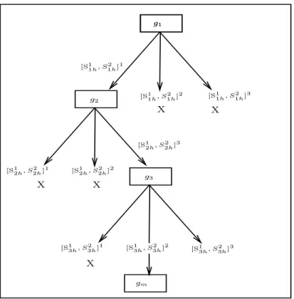
Algorithm 3 explains our proposed induction approach through a recur-sive process to generate the classification model. The tree is constructed in a top-down recursive divide-and-conquer manner, where each branch repre-sents the generated intervals for each attribute. The branches are selected recursively to compose the prototypes based on the proposed threshold . See Fig. 2 which explains graphically the proposed induction approach based on a recursive procedure. In this example, the branches marked with X sign are not selected for composing the prototypes. Using the generated tree from
g1 [S1 1h, S 2 1h] 1 [S1 1h, S 2 1h] 2 [S1 1h, S 2 1h] 3 g2 [S1 2h, S 2 2h] 1 [S1 2h, S 2 2h] 2 [S1 2h, S 2 2h] 3 g3 [S1 3h, S 2 3h] 1 [S1 3h, S 2 3h] 2 [S1 3h, S 2 3h] 3 g1 gm X X X X X
Figure 2: PROAFTN Decision Tree.
Fig. 2 we can extract the prototypes and then the decision rules respectively to be used for classification. Fig. 3 illustrates the prototype composition process. By applying Algorithm 3, we will be able to obtain the prototypes in an optimized (near optimized) form. Accordingly, these prototypes, as well as the testing dataset, can then be submitted to PROAFTN to start the classification process.
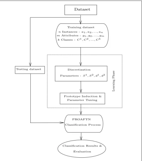
The general proposed methodology that summarizes the aforementioned Algorithms (1, 2, and 3) is represented in Fig. 4.
(bh1), Class: C h g1: [S 1 1h, S 2 1h] 1 g2: [S 1 2h, S 2 2h] 3 g3: [S3h1 , S3h2 ]2 gm: [S1mh, Smh2 ]k (bh2), Class: C h g1: [S 1 1h, S 2 1h] 1 g2: [S 1 2h, S 2 2h] 3 g3: [S 1 3h, S 2 3h] 3 gm: [Smh1 , S2mh]k (bhLh), Class: C h g1: [S 1 1h, S 2 1h] i g2: [S 1 2h, S 2 2h] i g3: [S 1 3h, S 2 3h] i gm: [Smh1 , Smh2 ]k
Figure 3: PROAFTN Prototypes.
5
Application and Analysis of the Developed
Algorithm
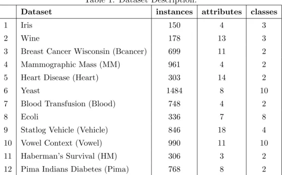
We have applied the above proposed Algorithms (1, 2, and 3) to 12 popular datasets presented in Table 1. The datasets are available on the public domain of the University of California at Irvine (UCI) Machine Learning Repository database [3]. Algorithms (1, 2, and 3) are all coded in java and run on Dell-Intel(R) Core(TM)2 CPU 2.13 GHz, 1.99 GB of RAM. To compare our proposed approaches with other machine learning algorithms, we have used the open source platform Weka [48] to run other algorithms such as C4.5 decision tress (DT), Naive Bayes (NB), Support Vector Machine (SVM), Neural Networks (NN), K-nearest neighbor (K-nn), and One-R [48]. The comparisons and evaluations are made on the same datasets and using 10 fold cross-validation [48].
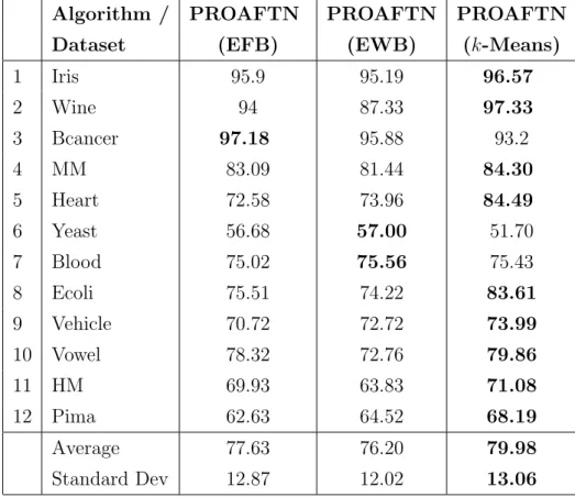
Our comparative study based on experimental results consists of two stages. The first stage presents the results obtained when applying the discretization techniques with PROAFTN to the datasets. This includes a comparison between the three proposed discretization techniques (k-Means, EWB, and EFB) based on classification accuracy. In the second stage, a gen-eral comparison is made between the generated results using our proposed methodology and those provided by C4.5, NB, SVM, NN, 1-nn, and One-R. Table 2 presents the classification accuracy generated by the application of discretization techniques (k-Means, EWB, and EFB) for PROAFTN on
Algorithm 3 : Building the classification model for PROAFTN. • Propose of a threshold β as reference for interval selection • For each class Ch, h = 1, 2, ..., k and for each attribute g
j, j =
1, 2, ..., m:
• Step 1: Choose the best branch (interval): [S1 jh, S
2
jh] from each attribute
gj as follows:
– If the percentage of values within this interval is ≥ β: ∗ Choose this interval to be part of the prototype bh
i
∗ Extend the tree recursively by adding a new branch from the next attribute gj+1 by going to Step 1
– Otherwise
∗ Discard this interval, and recursively go back to Step 1 to find another interval from the current attribute gj
• Step 2 (Prototype composition): The selected branches from attribute 1 to attribute m represent the induced prototypes for the class Ch
the proposed datasets. According to these results based on an average of clas-sification accuracy, using k-Means to obtain PROAFTN intervals generally generates better results than using EWB and EFB.
Some additional comments may be made on the previous experiments: - The use of k-Means for finding local minima is a good approach. k-Means uses more iterations to converge the near optimal solution compared to EFB and EWB.
- EFB is also a good approach in finding proper intervals for PROAFTN. As summarized in Table 2, EFB obtains good results in general because it is very good for data scaling; the objects are evenly divided on all bins, therefore preventing some values from dominating the classification process. Each of these methods (k-Means, EFB, and EWB) thus produce the best results in certain situations (dataset); we apply these approaches and choose the best result in each case to compare with the results provided by other classifiers. In Table 3 the results obtained on the same datasets by using the afore-mentioned machine learning techniques are compared with the best results
generated by PROAFTN. Based on the average of the classification accuracy measure illustrated in Table 3, we notice that NN is the best classifier overall. The performance of classifiers in descending order of accuracy is as follows: NN, PROAFTN, SVM, C4.5, NB, 1-nn, and One-R. PROAFTN is thus the closest in performance to NN.
However, according to Demˇsar [18], the comparative study based solely on the average of classification accuracy is limited and debatable for the following main reasons:
Dataset Training dataset Testing dataset mAttributes : g1, g2, ..., gm nInstances : a1, a2, ..., an kClasses : C1 , C2, ..., Ck PROAFTN
Classification Results & Evaluation Discretization
Prototype Induction & Parameter Tuning Parameters : S1 , S2 , d1 , d2 Classification Process L ea rn in g P h as e
Table 1: Dataset Description.
Dataset instances attributes classes
1 Iris 150 4 3
2 Wine 178 13 3
3 Breast Cancer Wisconsin (Bcancer) 699 11 2
4 Mammographic Mass (MM) 961 4 2
5 Heart Disease (Heart) 303 14 2
6 Yeast 1484 8 10
7 Blood Transfusion (Blood) 748 4 2
8 Ecoli 336 7 8
9 Statlog Vehicle (Vehicle) 846 18 4
10 Vowel Context (Vowel) 990 11 10
11 Haberman’s Survival (HM) 306 3 2
12 Pima Indians Diabetes (Pima) 768 8 2
• The different datasets have different characteristics, and therefore the use of only average classification results for comparisons might be mean-ingless.
• The average is also susceptible to outliers. The high performance of one classifier on one dataset may compensate for the bad performance of this classifier on other datasets.
Based on these factors related to the disadvantages of using the averages of classification accuracy of multiple classifiers over multiple datasets, we introduce the Friedman test with the corresponding post-hoc recommenced by Demˇsar [18] and (Garca and Herrera) [27]. The Friedman test enables for robust statistical comparisons of more classifiers over multiple datasets [18]; it ranks the algorithms for each dataset separately, the best performing algorithm getting the rank of 1, the second best the rank of 2, and so on.
The Friedman and Iman-Davenport tests use the χ2
and the F statistical distributions to determine if a distribution of the experimental frequencies differs from the theoretical expected frequencies. For more details about the Friedman and Iman-Davenport tests please refer to the following refer-ence [18]. The algorithm ranking of our experimental work based on applying
Table 2: Classification accuracy (in %) based on the application of discretiza-tion techniques for PROAFTN.
Algorithm / PROAFTN PROAFTN PROAFTN
Dataset (EFB) (EWB) (k-Means)
1 Iris 95.9 95.19 96.57 2 Wine 94 87.33 97.33 3 Bcancer 97.18 95.88 93.2 4 MM 83.09 81.44 84.30 5 Heart 72.58 73.96 84.49 6 Yeast 56.68 57.00 51.70 7 Blood 75.02 75.56 75.43 8 Ecoli 75.51 74.22 83.61 9 Vehicle 70.72 72.72 73.99 10 Vowel 78.32 72.76 79.86 11 HM 69.93 63.83 71.08 12 Pima 62.63 64.52 68.19 Average 77.63 76.20 79.98 Standard Dev 12.87 12.02 13.06
the Friedman test is shown in Table 4. Average ranks of the algorithms en-able a fair comparison among them. On average, NN, SVM, PROAFTN, and NB ranked in the first group (with ranks 2.37, 2.79, 3.58, and 3.71, respec-tively), and the second group was composed of C4.5, 1-nn, and OneR (with 4.17, 5.38, 6.0). The Friedman test checks whether the measured average ranks are significantly different from the mean rank Rj = 4.
In some cases, we need to identify the pairwise difference among the clas-sifiers. For this reason we need to proceed with the post-hoc tests to measure and detect these differences. In this paper, we consider the following corre-sponding statistics procedure including Holm, Hochberg, Nemenyi, Shafer, and Hommel [18, 27]. For this type of comparisons, we have to compute and order the aforementioned corresponding statistics and p-value and the standard error SE.
Table 3: Experimental results based on classification accuracy (in %) to mea-sure the performance of the different classifier compared with PROAFTN.
Algorithm / C4.5 NB SVM NN 1-nn One-R PROAFTN Dataset 1 Iris 96.00 96.00 96.00 97.33 95.33 94.00 96.57 2 Wine 91.55 97.40 99.35 97.40 95.45 69.48 97.33 3 Bcancer 94.56 95.99 96.70 95.56 95.85 91.55 97.18 4 MM 82.10 78.35 79.24 82.10 75.03 81.89 84.30 5 Heart 76.60 83.70 84.10 78.10 75.19 71.11 84.49 6 Yeast 56.00 57.61 57.08 59.43 52.29 40.16 57.00 7 Blood 77.81 75.40 76.20 78.74 69.12 76.07 75.56 8 Ecoli 84.23 85.42 84.23 86.01 80.36 63.69 83.61 9 Vehicle 72.58 44.80 74.47 82.51 69.86 51.54 73.99 10 Vowel 82.53 67.88 68.59 82.53 99.09 32.22 79.86 11 HM 71.90 74.83 73.52 72.87 67.65 73.02 71.08 12 Pima 71.48 75.78 77.08 75.39 71.48 71.35 68.19 Average 79.78 77.76 80.55 82.33 78.89 68.01 80.76 Standard Dev 11.34 15.82 12.40 11.01 14.58 18.79 12.50
Table 4: Average Rankings of all algorithms including PROAFTN in the study over the proposed datasets, based on the classification accuracy by using 10-fold cross validation.
Algorithm Ranking NN 2.37 SVM 2.79 PROAFTN 3.58 NB 3.71 C4.5 4.17 1-nn 5.38 OneR 6.0
Table 5 presents the hypotheses ordered by their p-value and the adjust-ment of α’s by Holm’s, Hochberg’s, and Hommel’s statistical procedures.
Friedman’s and Iman-Davenport’s statistics are respectively: • χ2
= 26.4286 distributed with 6 degrees of freedom, • F = 6.3793 distributed with 6 and 66 degrees of freedom.
Table 5: Holm / Hochberg Table for α = 0.05. i algorithm z = (R0− Ri)/SE p 1 OneR 4.1103 3.9503E-5 2 1-nn 3.4016 6.6972E-4 3 C4.5 2.0315 0.0421 4 NB 1.5118 0.1305 5 PROAFTN 1.3701 0.1706 6 SVM 0.4724 0.6366
• Holm’s procedure rejects the hypotheses 1 and 2 since the correspond-ing p-value ≤ 0.0125 the adjusted α’s.
• Hochberg’s procedure rejects those hypotheses 1 and 2 since they have the p-value ≤ 0.01.
• Hommel’s procedure rejects those hypotheses 1 and 2 since the p-value ≤ 0.0125.
Based on these results we can identify that the classifiers OneR and 1-nn are significantly worse than NN and SVM based on p-value. We also can recognize that PROAFTN is next to SVM in performance compared with NN; hence, there is no significant difference in performance between NN and PROAFTN.
To detect the pairwise comparisons between PROAFTN and the other algorithms, we proceeded to use other corresponding measures such as Ne-menyi’s and Shaffer’s statistics procedures. Table 6 presents the family of hypotheses sorted by their p-value and the adjustment of α’s by Nemenyi’s, Shaffer’s, and Holm’s procedures. In this experiment we were only concerned with comparing PROAFTN with other classifiers, so only the rows that in-clude PROAFTN are inin-cluded in this analysis.
• Nemenyi’s procedure rejects those hypotheses that have a p-value ≤ 0.0023.
• Holm’s procedure rejects those hypotheses that have a p-value ≤ 0.0027. • Shaffer’s procedure rejects those hypotheses that have a p-value ≤
0.0023.
The results presented in Table 6 show the relative performance of PROAFTN against other classifiers.
Table 6: Holm / Shaffer Table for α = 0.05
i algorithms z = (R0− Ri)/SE p α Holm α Shaffer
1 OneR vs. PROAFTN 2.740 0.006 0.003 0.003 2 1-nn vs. PROAFTN 2.032 0.042 0.004 0.004 3 NN vs. PROAFTN 1.370 0.171 0.006 0.006 4 SVM vs. PROAFTN 0.898 0.369 0.008 0.008 5 C4.5 vs. PROAFTN 0.661 0.508 0.013 0.013 6 NB vs. PROAFTN 0.142 0.887 0.05 0.05
According to the obtained results, we can clearly distinguish among three groups of classifiers, based on their performance:
• Best classifiers: NN, SVM, PROAFTN. • Middle classifiers: NB and C4.5.
• Worst classifier: OneR and 1-nn.
To sum up, we conclude from the discussed analysis and results that respectively NN, SVM, and PROAFTN generally obtain the best results overall. NN employees optimization techniques and intensive incremental learning to obtain optimal classification accuracy [14]. The goal of this it-erative learning process in NN is to seek the optimal weights that improve the classification accuracy in each iteration. SVM also uses optimization approaches to find the best hyperplane to separate the objects belonging to each class [13, 39]. On the other hand, PROAFTN requires some parameters and uses fuzzy approach to assign the objects to the classes. As a result there is richer information, more flexibility and greater accuracy in assigning the objects to the right class.
6
Discussions and Conclusions
In this paper, we proposed a new classification methodology that utilizes ma-chine learning techniques to learn and improve the Multi-Criteria Decision Analysis (MCDA) method PROAFTN. The major advantages of MCDA could be summarized as: (i) explaining the classification results, therefore avoiding black box situations, and (ii) interrogation of the decision-maker and preferences. In some cases we do not have the decision-maker, only the dataset; in these cases, we need an automatic approach to infer preference parameters. In this paper we used discretization techniques to automatically infer these parameters from the dataset to learn PROAFTN. After this pro-cess, we proposed an induction approach to obtain the best prototypes that construct the classification model to classify new data.
The comparison of experimental results was based on advanced statistical approaches, including Friedman and other corresponding statistics measures. The obtained results based on each dataset show that our proposed approach to PROAFTN gives better results than One-R, 1-nn, C4.5, and NB, and in some cases better than SVM and NN. The major property of PROAFTN is the ability to generate the decision-rules through learning to be used later by the decision-maker. PROAFTN also allows the introduction of human judgment (expert) in setting PROAFTN preferences (intervals and weights). Thus, the PROAFTN parameters can be determined in three different ways: using the training dataset - as presented in this article -, experts, or both at the same time. We believe that with the introduction of human judgment and the use of optimization approaches to obtain optimal parameters, PROAFTN results can be further improved.
PROAFTN also possesses a number of particular strengths compared with other well-known classifiers, such as: (i) PROAFTN results are auto-matically explained, which provides the possibility of access to more detailed information concerning the classification decision. Regarding objects’ as-signment, the fuzzy membership degree gives us an idea about their “weak” and “strong” membership in the corresponding classes; (ii) PROAFTN takes into consideration the interdependency between attributes compared with NB. This property is important especially when the attributes are highly de-pendent on each other, such as in the case of medical data; (iii) PROAFTN can be used to perform two learning paradigms, deductive and inductive learning, and is thus the ideal method for combining prior knowledge and data; and (iv) PROAFTN does not require any reprocessing or
transforma-tion of data. The classificatransforma-tion procedure is based on pairwise comparisons, which eliminates any problem involved with different measurement units of attributes.
Many improvements could be made to enhance PROAFTN to achieve better classification accuracy, including the following:
• Integrate the attribute weights in the learning process. In this presented article we assumed all attributes have the same influence and equals to 1 in the classification procedure. The future stage of this research is to investigate other approaches to include the weights’ impact in the learning and classification process, thus recognizing the best attributes and degrading the influence of weak ones.
• Exploit the optimization approach [49], mainly metaheuristics such as Tabu search [28], Genetics Algorithms [42], and Variable Neighbor-hood Search (VNS) [30], to infer the optimal parameters from training datasets during the learning process.
Acknowledgment
We gratefully acknowledge the support from NSERC’s Discovery Award (RGPIN293261-05) granted to Dr. Nabil Belacel.
References
[1] R. Agrawal, T. Imielinski, and A. Swami. Database mining: A perfor-mance perspective. IEEE Trans. Knowledge and Data Eng, 5(6):914– 925, 1993.
[2] A. An and N. Cercone. Discretization of continuous attributes for learn-ing classification rules. Third Pacific-Asia Conference on Methodologies
for Knowledge Discovery & Data Mining, pages 509–514, 1999.
[3] A. Asuncion and D.J. Newman. UCI machine learning repository, 2007. [4] P.W. Baim. A method for attribute selection in inductive learning sys-tems. IEEE Transactions on Pattern Analysis and Machine Intelligence, 10(6):888–896, 1988.
[5] N. Belacel. Multicriteria Classification methods: Methodology and
Medi-cal Applications. PhD thesis, Free University of Brussels, Belgium, 1999.
[6] N. Belacel. Multicriteria assignment method proaftn: methodology and medical application. European Journal of Operational Research, 125(1):175–183, 2000.
[7] N. Belacel and M. Boulassel. Multicriteria fuzzy assignment method: A useful tool to assist medical diagnosis. Artificial Intelligence in Medicine, 21(1-3):201–207, 2001.
[8] N. Belacel, H. Raval, and A. Punnen. Learning multicriteria fuzzy classi-fication method proaftn from data. Computers and Operations Research, 34(7):1885–1898, 2007.
[9] N. Belacel, P. Vincke, M. Scheiff, and M. Boulassel. Acute leukemia di-agnosis aid using multicriteria fuzzy assignment methodology. Computer
Methods and Programs in Biomedicine, 64(2):145–151, 2001.
[10] N. Belacel, Q. Wang, and R. Richard. Web-integration proaftn method-ology for acute leukemia diagnosis. TELEMEDICINE AND e-HEALTH, 11(6):1885–1898, 2005.
[11] G. Brassard and P. Bratley. Fundamentals of Algorithms. Prentice Hall, 1996.
[12] I. Bruha. From machine learning to knowledge discovery: Survey of preprocessing and postprocessing. Intelligent Data Analysis, 4:363–374, 2000.
[13] C. Burges. A tutorial on support vector machines for pattern recogni-tion. Data Mining and Knowledge Discovery, 2(2):1–47, 1998.
[14] G. Castellano, A. Fanelli, and M. Pelillo. An iterative pruning algo-rithm for feedforward neural networks. IEEE Transactions on Neural
Networks, 8(3):519–531, 1997.
[15] J. Cheng, R. Greiner, J. Kelly, D. Bell, and W. Liu. Learning bayesian networks from data: An information-theory based approach. Artificial
[16] G. Cooper and E. Herskovits. A bayesian method for the induction of probabilistic networks from data. Machine Learning, 9(4):309–347, 1992.
[17] K. Crammer and Y. Singer. On the learnability and design of output codes for multiclass problems. Machine Learning, (47):201–233, 2002. [18] Janez Demˇsar. Statistical comparisons of classifiers over multiple data
sets. J. Mach. Learn. Res., 7:1–30, 2006.
[19] L. Dias, V. Mousseau, J. Figueira, and J. Climaco. An aggrega-tion/disaggregation approach to obtain robust conclusions with electre tri. European Journal of Operational Research, 138(2):332–348, 2002. [20] F. Divina and E. Marchiori. Handling continuous attributes in an
evolu-tionary inductive learner. in IEEE Transactions on Evoluevolu-tionary
Com-putation, 9(1):31–43, 2005.
[21] M. Doumpos and C. Zopounidis. The use of the preference disaggre-gation analysis in the assessment of financial risks. Fuzzy Economic
Review, 3(1):39–57, 1998.
[22] R. O. Duda, P. E. Hart, and D. G. Stork. Pattern Classification (2nd
ed.). John Wiley & Sons, 2001.
[23] D.M. Dutton and G.V. Conroy. A review of machine learning. The
Knowledge Engineering Review, 12:4:341–367, 1996.
[24] U.M. Fayyad and K.B. Irani. Multi-interval discretization of continuous-valued attributes for classification learning. XIII International Joint
Conference on Artificial Intelligence (IJCAI93), pages 1022–1029, 1993.
[25] U.M. Fayyad and R. Uthurusamy. Evolving data mining into solutions for insights. Comm. ACMg, 45(8):28–31, 2002.
[26] A. Freitas. Data Mining and Knowledge Discovery with Evolutionary
Algorithms. Springer, 2002.
[27] Salvador G. and Francisco H. An extension on “statistical comparisons of classifiers over multiple data sets” for all pairwise comparisons. Journal
[28] F. Glover and M. Laguna. Tabu Search. Kluwer Academic Publishers, 1997.
[29] M. Goebel and L. Gruenwald. A survey of data mining and knowledge discovery software tools. SIGKDD Explor. Newsl, 1(1):20–33, 1999. [30] P. Hansen and N. Mladenovic. Variable neighborhood search for the
p-median. Location Science, 5:207–226, 1997.
[31] K. Jabeur and A. Guitouni. A generalized framework for concordance/discordance-based multi-criteria classification methods.
Information Fusion, 2007 10th International Conference 9-12 July 2007,
pages 1–8, 2007.
[32] S. Kotsiantis and D. Kanellopoulos. Discretization techniques: A recent survey. GESTS International Transactions on Computer Science and
Engineering, 32(1):47–58, 2006.
[33] S.B. Kotsiantis. Supervised machine learning: A review of classification techniques. Informatica, (31):249–268, 2007.
[34] O. Larichev and H. Moskovich. An approach to ordinal classification problems. International Transactions in Operational Research, 1(3):375– 385, 1994.
[35] D.T. Larose. Discovering Knowledge in Data: An Introduction to Data
Mining. John Wiley & Sons, 2005.
[36] J. Lger and J-M. Martel. A multi-criteria assignment procedure for a nominal sorting problematic. European Journal of Operational Research, 138:349–364, 2002.
[37] T. Mitchell. Machine Learning. McGraw Hill, 1997.
[38] K. Nigam, A. Mccallum, S. Thrun, and T. Mitchell. Text classification from labeled and unlabeled documents using em. Machine Learning, 39:103–134, 2000.
[39] S. Pang, D. Kim, and S.Y. Bang. Face membership authentication using svm classification tree generated by membership-based lle data partition.
[40] C. Pinto and J. Gama. Partition incremental discretization. In
Pro-ceedings of 2005 Portuguese Conference on Artificial Intelligence, pages
168–174. IEEE Computer Press, 2005.
[41] D. Pyle. Data Preparation for Data Mining. Morgan Kaufmann Pub-lishers, 1999.
[42] C. R. Reeves and J. E. Rowe. Genetic Algorithms: Principles and
Per-spectives. A Guide to GA Theory. Kluwer Academic Publishers, 2002.
[43] B. Roy. Multicriteria methodology for decision aiding. Kluwer Academic, 1996.
[44] P. Smyth, D. Pregibon, and C. Faloutsos. Data-driven evolution of data mining algorithms. Comm. ACM, 45(8):33–37, 2002.
[45] M. Snow, R. Fallat, W. Tyler, and S. Hsu. Pulmonary consult: Concept to application of an expert system. Journal of Clinical Engineering, 13(3), 1988.
[46] F.J. Sobrado, J.M. Pikatza, I.U. Larburu, J.J. Garcia, and D. de Ipi˜na. Towards a clinical practice guideline implementation for asthma treat-ment. In R. Conejo, M. Urretavizcaya, and J. P´erez-de-la Cruz, editors,
Current Topics in artificial intelligence: 10th conference of the Spanish association for artificial intelligence, Lecture notes in computer science,
pages 587–596. Springer, Heidelberg, 2004.
[47] S. Weiss and C. Kulikowski. Computer Systems That Learn-Classification and Prediction methods from Statistics, Neural Nets, Ma-chine Learning and Expert Systems. Morgan-Kaufmann, 1991.
[48] H. Witten. Data Mining: Practical Machine Learning Tools and
Tech-niques. Morgan Kaufmann Series in Data Management Systems, 2005.
[49] M. Yagiura and T. Ibaraki. On metaheuristic algorithms for combinato-rial optimization problems. Systems and Computers in Japan, 32(3):33– 55, 2001.
[50] C. Zopounidis and M. Doumpos. Building additive utilities for multi-group hierarchical discrimination: The m.h.dis method. Optimization
[51] C. Zopounidis and M. Doumpos. Multicriteria preference disaggregation for classification problems with an application to global investing risk.
Decision Sciences, 32(2):333–385, 2001.
[52] C. Zopounidis and M. Doumpos. Multicriteria classification and sort-ing methods: A literature review. European Journal of Operational