ACCURACY FOR HYDRAULIC FRACTURING AT
THE DWTI SITE, JASPER, TEXAS
Shirley Rieven and William Rodi
Earth Resources Laboratory
Department of Earth, Atmospheric, and Planetary Sciences
Massachusetts Institute of Technology
Cambridge, MA 02139
ABSTRACT
This report presents the results of a feasibility study designed to assess whether mi-croseismic location techniques can provide enough accuracy and precision to enable a high resolution study of the spatial distribution of microseismic events induced during a hydraulic fracture experiment. We calculated the 90% confidence regions for six syn-thetic microevent 'clusters' along the azimuth of a hydraulic fracture produced during Atlantic Richfield's 1993 Fracture Technology Field Demonstration Project in Jasper, Texas. Examination of the confidence regions for the absolute locations indicates that microseismic events can be confidently located for areas near the monitoring wells but away from the plane intersecting the two observation points. We determined that the resolution for events located at the ends of the fracture is poor but improves dramati-cally nearer the wells. The minimum dimensions of the 90% confidence regions for events within our study area are approximately 8 ft in the northwest-southeast direction, 3 ft in the northeast-southwest direction, and 3 ft in depth.
INTRODUCTION
Delineating the spatial distribution of hydraulically-induced fractures has been the sub-ject of active research for over twenty years, particularly as it applies to exploration for oil, natural gas and geothermal energy resources. Recovery of resources from a reservoir may require stimulation of these fractures, therefore a thorough understanding of their interaction is crucial to an effective design. The methods used to determine the basic fracture parameters of height, azimuth and width have evolved over the years and have
included such disparate techniques as shear acoustic anisotropy, anelastic strain recov-ery (ASR), overcoring of microfracs, natural and coring induced core fractures, borehole microseismic monitoring, and borehole televiewer imaging. Microseismic monitoring is unique among these techniques in thatit is the only method capable of resolving, in a non-invasive manner, the macroscopic three-dimensional structure of the fracture at significant distances from the borehole. This method is not vulnerable to disturbances associated with core recovery (a particular problem in unconsolidated materials) and has been shown to compare favorably in accuracy to several of the best methods, specifically ASR, and overcoring (Yale et al., 1992). The emergence of advanced sensor technol-ogy for microboreholes will impact the cost/benefit of this method bringing it into a more favorable position with respect to the alternative techniques. This development presents a unique opportunity to more clearly determine the parameters governing the shape of hydraulic fractures under field conditions and to improve our confidence in the hypocenter locations derived from the associated induced microseismicity.
A variety of methods have been used to determine the hypocentral location coor-dinates and origin times of microseismic events induced by hydraulic fracturing. Prior to the early 1980s, the hypocenters and origin times were commonly determined using variations of Geiger's method and alternatively, the 3-point method originally intro-duced by Lutz in 1986 (Fehler et al., 1987). Later developments incorporated the use of relative event location techniques to locate microearthquakes that are closely placed in space. These techniques were later expanded to include the use of cross-spectral, moving-window methods to make use of the similarity of related events called dou-blets (Frechet et al., 1989; Frankel, 1982; Geller and Mueller, 1980; Poupinet et al., 1984; Thornjarnardottir and Pechmann, 1987; Fremont and Malone, 1987; Deichmann and Garcia-Fernandez, 1992; Moriya et al., 1994).
This paper presents an evaluation of the microseismic location accuracy for a solid waste disposal demonstration project conducted by Atlantic Richfield Corporation. The microseismic activity was monitored using 150 downhole geophones, making this exper-iment one of the most heavily instrumented to date. This high receiver density presents an excellent opportunity to study the fracturing process in greater detail than has been attempted using data from sparser arrays. We are particularly interested in the occur-rence of seismicity away from the plane of the fracture. Traditional treatment of the hydraulic fracture process predicts rupture along a planar fracture due to tensile effec-tive stresses, yet, past seismic monitoring of hydrofracture experiments have suggested the occurrence of microseismicity away from the predicted plane. Our immediate goal is to determine whether the accuracy of our location technique is sufficient to investigate these remote rupture processes. We begin by assessing our location algorithm's ability to spatially resolve the hypocenters. To this end, we determined the 90% confidence regions for 6 grids of synthetic hypocenters by forward modeling the P and S wave trav-eltimes to the known locations of the seismic receivers used in the demonstration. We synthesized picking errors by adding distance-weighted random noise and then inverting for the absolute hypocenter parameters. We used this procedure to evaluate the lateral
variation of the confidence regions so as to quantify the maximum resolution attainable from the DWTI data.
THE FRACTURE TECHNIQUES TECHNOLOGY FIELD DEMONSTRATION PROJECT
Atlantic Richfield's Deep Well Treatment and Injection Program Atlantic Richfield Corporation (ARCO) proposed that solid waste could be safely dis-posed of by suspending the solids in a bentonite slurry and injecting them into deeply buried, hydrogeologically isolated formations. ARCO presented the method and its safe application in a Fracture Technology Field Demonstration conducted over a five day period in October 1993 at the Deep Well Treatment and Injection Site (DWTI) in Jasper, Texas (Figure 1). During the demonstration, ARCO injected 4 million pounds of sand and bentonite clay and 2.1 million gallons of water into an isolated portion of the Lower Frio Sand. The injection was conducted in four segments designated as cycles 0, 1, 2, and 3. These injection cycles hydraulically fractured the sand while forcing the sand/clay suspension into the fractured zone and surrounding formation. The demon-stration specifically addressed two key issues concerning the disposal method: (1) the technique must be able to dispose of a significant quantity of waste; and (2) the zone of disposal must be known to ensure containment of the wastes within the isolated forma-tion. The answer to the first issue was given immediately by the amount of simulated waste injected during the demonstration. The second issue was addressed in two parts. First, ARCO showed that the fracture growth could be monitored in real time by lo-cating microseismic events induced by the fracture. Second, they demonstrated that the fracture dimensions determined by microseismic monitoring were in agreement with those predicted by currently available fracture modeling methods and that the results from both methods suggested that the fracture had not compromised the integrity of the confining layers (Atlantic Richfield Corporation, 1994).
Geologic Environment
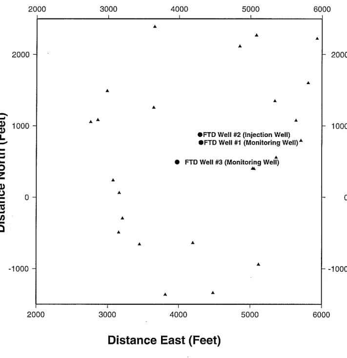
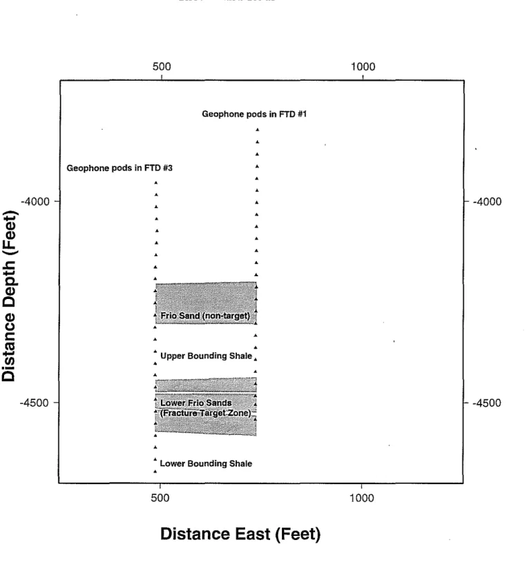
ARCO produced the DWTI hydraulic fracture by injecting the simulated waste into an isolated sand layer via a well designated the Field Technology Demonstration Well #2 (FTD #2). Simultaneously, microseismic events were recorded by geophones lo-cated in two monitoring wells designated FTD Wells #1 and #3. Figure 2 shows the field geometry of the three wells. The injection well (FTD #2) was constructed using standard petroleum field completion with the perforation extending from 4426-4614 ft. ARCO placed the perforation so that the geologic unit receiving the waste was a 155 ft thick portion of the Lower Frio Sand (Figure 3). This section of the Lower Frio Sand is bounded above by a 130 ft thick layer of shale and below by a 1500 ft thick layer of shale. The Lower Frio Sand is regionally continuous and of large lateral extent. The nearest known fault is at a distance of 5000 ft away from the perforated zone (ARCO,
1994). The perforation extends slightly below the top of the lower bounding shale, but due to the very large vertical extent of this unit, the slight intrusion did not pose a difficulty for the disposal demonstration.
Seismic Receiver Geometry
ARCO placed 150 30-Hertz geophones in the two monitoring wells to record the mi-croseismic activity during the injection. Two strings of 75 geophones (25 pods, each containing three orthogonally-oriented phones) were installed-one string in each of the two monitoring wells (FTD #1 and #3). The 25 pods were located along the strings at 30 ft intervals over a range spanning the target sand layer and portions of the upper and lower bounding shales. The full string of phones provided a total aperture of 720 ft for each well (Figure 3). ARCO located each pod vertically by radioactive tracers, but the absolute orientation of the two horizontal phones in each pod has not been determined. The Frio Sand is a permeable, unconsolidated layer prone to washouts; therefore, the geophone strings were cemented inside the casings. The microseismic activity was sam-pled continuously at a rate of 2000 samples per second and detected events were isolated and saved as separate event files. Approximately 2400 individual events were recorded during the five-day demonstration.
ARCO chose the lateral location of the monitoring wells based upon the predicted azimuth of the fracture as determined from various lab and field experiments. Hydraulic fractures, induced at depth from non-deviated wellbores, propagate perpendicular to the direction of least principal stress. Therefore, three separate laboratory tests were con-ducted on cores from FTD Well #1 to determine this direction. These tests included Anelastic Strain Recovery (ASR), Differential Strain Curve Analysis (DSCA), and Ve-locity Anisotropy (VELAN). ASR predicted the least principal stress as being N35E ± 5°, DSCA predicted the direction to be N12E to N40E, and VELAN predicted the direction to be N35E ± 5°. Televiewer inspection of borehole breakouts indicated a minimum stress direction of N45E
±
30°, while examination of the strikes of nearby growth faults indicated that the regional minimum stress direction was N80E±
20°. Because of the amount of disagreement between these estimates, ARCO conducted a microfrac test (fracture azimuth injection test). The azimuth of the fracture induced during this test was monitored using a surface array of tiltmeters (Figure 2). The final estimate of fracture azimuth was taken to be N40E. Based upon a combination of these test results, the monitoring wells were installed such that the expected azimuth of the fracture bisected both wells. Despite the preliminary estimates, the DWTI fracture propagated N66E and thus did not bisect the two monitoring wells as expected. Due to the nature of the experiment and the large lateral extent of the Lower Frio Sand unit, the unexpected fracture azimuth had little effect on the objective of the demon-stration. These difficulties, however, illustrate the difficulty in determining accurate fracture propagation parameters.DWTI
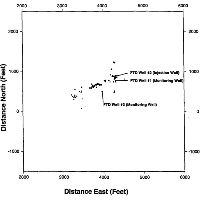
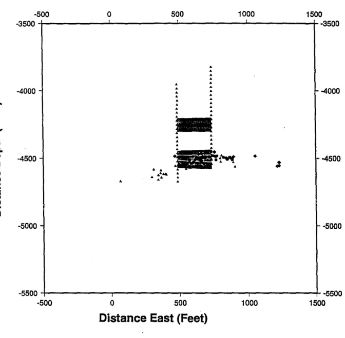
Fracture GeometryDuring the hydraulic fracturing, microseismicity was recorded by 96 of the 150 available geophones via ARCO's Digital Acquisition System. In addition to being saved as an independent file, each detected event was examined to determine which geophone along the string triggered first. Based upon the vertical receiver geometry and the concept of minimum traveltime, a preliminary estimate of the hypocentral depth was determined. This method allowed a real-time assessment of vertical fracture growth, accurate to one-half of the pod spacing (15 ft) which was accurate enough (relative to the vertical extent of the bounding shale layers) to determine whether the microseismicity was confined within the sand layer (as predicted by the mathematical fracture algorithms). The real time estimates were suggested that the fracture had, indeed, stayed within the target zone, and this assessment was further supported by subsequent, more precise locations determined for the 100 largest magnitude events using an inversion algorithm developed by Los Alamos National Laboratory (House, 1987). Figures 4 and 5 show the epicentral and depth locations of these 100 events (as located by ARCO).
FORWARD MODELING OF SYNTHETIC MICROEVENT
CLUSTERS
The objective of this study was to assess the lateral variation of the 90% confidence regions for the hypocenters of hypothetical (synthetic) microearthquake clusters located along the azimuth of the DWTI hydraulic fracture. Figures 6 and 7 show six synthetic event clusters with two different inter-event spacings-50 ft and 100 ft-upon which we conducted our numerical experiments. In the following sections we present the method used to calculate the hypocenter coordinates and the results of the accuracy and spatial variation tests.
Method for Determining Hypocenter Location
Our event relocation method fits the hypocenters and origin times of a set of events in a cluster simultaneous to a set of absolute and differential arrival time data observed at various stations. The absolute arrival time for an event e, station s and wave type w (P or S) is modeled as
(1)
Here, Xe is the hypocentral coordinate vector and
t
e the ongm time of the event.The function F gives the theoretical traveltime between Xe and the station location x, through an assumed slowness model Uw' n"w denotes the observational error in T"w' Differential arrival times between a "slave" event e and a "master" event rare modeled as
Note that the observational error in a differential time is not a difference between ab-solute arrival time errors, because we assume that !1Tresw has been measured
indepen-dently ofTesw andTrsw . An additional source of error occurs in both absolute and differ-ential times when the slowness modelsU w are not known exactly, e.g., a one-dimensional
approximate model is often assumed. Such "modeling errors" affect primarily absolute times and tend to cancel in differential times between closely spaced events. We solve equations (1) and (2) for the Xeand
te,
using available (e,s,w) and (r,e, s,w)combina-tions, by minimizing the errors nesw and nresw in a least squares sense using a conjugate
gradient algorithm (Rodi et al., 1993). Estimates of the errors in the predicted loca-tions are determined using linear approximaloca-tions and the statistical methods outlined by Jordan and Sverdrup (1981).
Forward Modeling of the P and S Wave Traveltimes With Noise
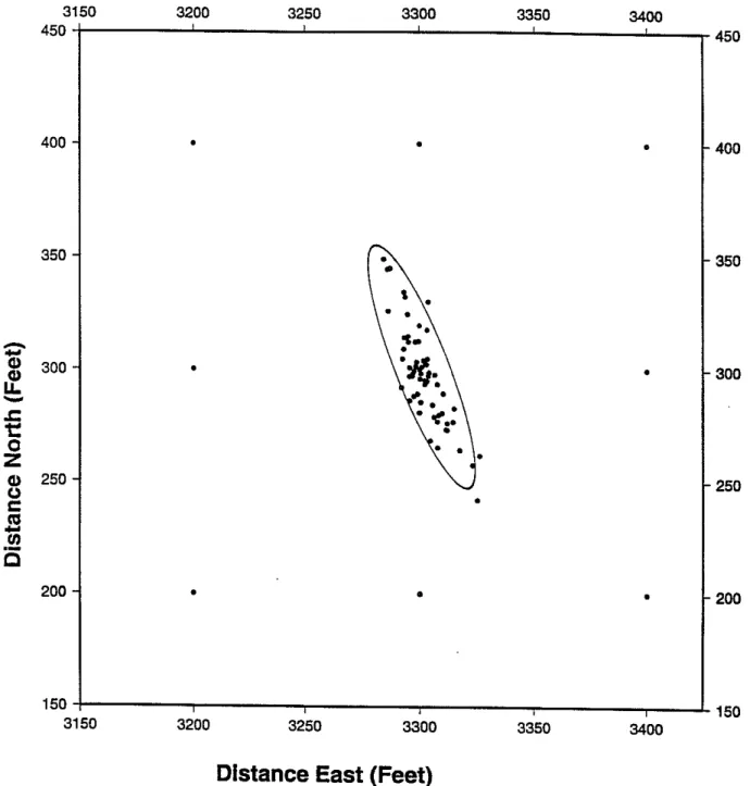
Vlfe calculated the P and S wave arrival times for the synthetic hypocenters shown in Figures 6 and 7 at a depth of 4500 ft, using a horizontally-layered velocity structure model with P wave velocities for the sand of 8100 ft/sec and S wave velocities of 3682.0 ft/sec. Shale P wave velocities were set to 7272.7 ft/sec, with shale S wave velocities of 3305.8 ft/sec. In calculating the arrival times, we specified picking error uncertainties derived from a linear dependence on horizontal distance between the hypocenter and the monitoring well. These errors were approximated by adding pseudo-random noise with a Gaussian distribution. We specified the standard deviations based upon ARGO's estimate of the picking error for the primacord shots (1 ms) and on RMS errors for previ-ously located events in cycle 2 (located near the farthest extent offracture propagation), 6ms. Figure 8 shows the results of a test conducted to confirm the accuracy of the 90% confidence regions for one of the synthetic hypocenters from Grid Ab (event Abyy). This figure shows the predicted hypocenters determined using 60 independent sets of noise. Fifty-four of the 60 hypocenter estimates (93%) fall within the 90% confidence region, demonstrating that the regions calculated for this study are correct. (The confidence region presented for comparison is taken from the most accurate relocated event of the 60 studied).
We tested the accuracy of our hypocenter location algorithm by comparing the location of the 90% confidence regions with the true location of the hypocenters. The results of this study are presented beginning with the grid furthest southwest (Grid A) and progressing toward the northeast. With this ordering, the confidence ellipses begin large, pass through the expected minimum size, and then increase again as we exit the area best covered by the receiver geometry. The ellipses determined for grids A through E (at 50 ft spacing) are shown in Figures 9-14. The circles plotted represent the true locations of the hypocenters, whereas the estimated hypocenters are at the center of the 90% confidence regions as estimated by the inversion algorithm. Additionally, we included the location of real hypocenters from the DWTI (as located by ARGO) to indicate the relative spacing between actual events. The confidence regions for grids D, E and F (Figures 12, 13, and 14) illustrate the poor confidences possible for areas
northeast of the wells. No further consideration of events in grids D, E, or F will be given based upon these results.
The results from the forward modeling for grids Aa-Ea quantify the spatial vari-ation in confidence regions over the length of the southwestern wing of the fracture (Figures 9, 10, and 11). The average maximum semi-axis for the events in this wing varies from a maximum of 55 ft (center of grid Aa) to 12 ft (center of grid Cal. The average minimum semi-axis for the events varies from a maximum of 11 ft (center of grid Aa) to 4 ft (center of grid Cal. The 90% confidence region for the depth axis varies from a maximum of 12 ft (center of grid Aa) to a minimum of 3 ft (center of grid Cal. All range values are rounded to the nearest foot. Itis also apparent that the geometry of the wells contributes to the characteristics of the confidence regions. The average azimuthal direction of the major axis varies spatially from N21.3W (grid A) to N8.5E (grid B), a clockwise rotation around the wells. For grids A and B, the wells are both located on the eastern side. The azimuth changes to N37.8W for grid C, located longitudinally between the two wells.
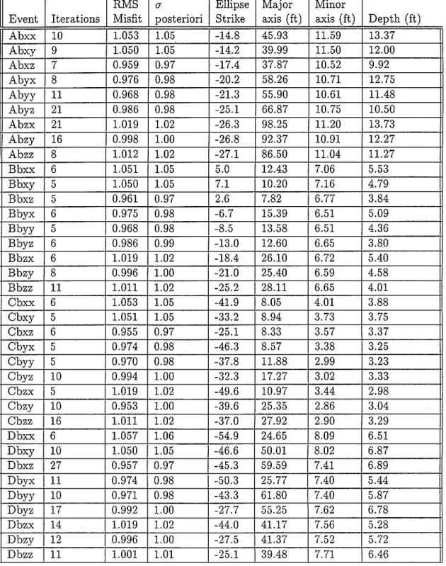
We also calculated the regions for grids with 100 ft spacing to evaluate the lateral variation in region size and orientation (Figures 15, 16, and 17). The results of the inversions for the 100 ft grids are presented quantitatively in Table 1. Convergence was commonly attained within 11 iterations of the conjugate gradient algorithm with final RMS misfits and average posteriori standard deviations of approximately 1.00. These results show the variation in the major semi-axis of the confidence regions as a function of distance away from the line connecting the two monitoring wells. Li and Thurber (1991) demonstrated that for receiver arrays with only two laterally separated monitoring locations, the spatial resolution is poor for events along the plane separating the observation points. We can observe this effect for the DWTI data by comparing the semi-major axes diagonally across the grids. This axis dimension increases by a factor of 1.88 for grid A, far from the intersecting plane, but by a factor of 3.47 for grid C, nearest the intersecting plane. We also observe the effect of distance from the plane by inspecting the change in ellipse azimuth across the grid. Grid A shows a variation of approximately 12.3° (clockwise rotation) between event Abzz and Abxx. Variations of 36.9° and 4.9° (counterclockwise), are observed for grids Band C, respectively.
We can use the 90% confidence regions predicted for grids A through C to qualita-tively determine the resolvability of events within the actual DWTI fracture zone, as determined from the events located by ARCO. It is clear from inspection of the semi-major axis dimensions for all three grids that the resolution in the northeast-southwest direction is good, especially for events located within the region covered by grid C. However, resolution of the hypocenter coordinates in the northwest-southeast direction varies considerably over the length of the extent of the fracture wing. Actual events from the early phases of the DWTI injection (cycle 1) were determined to be located within grid C (Figures 4, 6, and 7). These events are closely spaced but resolvable in many instances (Figures 16 and 17). The events induced during cycle 2 are less well-resolved, particularly in the northwest-southeast direction (Figure 15).
These results compare favorably with those found for other experiments of this type. For example, House (1987) located the hypocenters of805 microseismic events at the Fenton Hill Geothermal Field using similar techniques. These events were located with an accuracy of25 to 30 meters. Vinegar et al. (1992) estimated the accuracy of relative event location of events in a downhole experiment similar to the DWTI demonstration as being 1.5 ft radially and 1 ft vertically, but noted that absolute locations would be much greater.
CONCLUSIONS
The results of this study indicate that microseismic events induced by hydraulic frac-turing during the Atlantic Richfield Corporation Field Demonstration Project can be confidently located for areas near the monitoring wells but away from the plane inter-secting the two observation points. We determined that the minimum dimensions of the 90% confidence regions for events within our study area are approximately 8 ft in the northwest-southeast direction, 3 ft in the northeast-southwest direction, and 3 ft in depth.
The results of this study suggest that the resolution provided by the technique of absolute hypocenter location as it applies specifically to the Field Demonstration Ex-periment, are comparable to that found in other similar studies. However, we show that the area of good resolution excludes the extreme lateral extent of the fracture thus lim-iting the detail with which we can examine the fracture process. The location errors can be interpreted as the minimum distance between fractures that is resolvable using this technique. We anticipate that application of relative event location techniques to real data from the DWTI demonstration will improve the accuracy of the hypocenter loca-tions by reducing the arrival time picking errors and minimizing any effects of erroneous velocity model estimates. An analysis of the expected improvement will further define the minimum fracture separation resolvable in those areas not adequately addressed using absolute location techniques.
ACKNOWLEDGMENTS
We would like to thank Dr. Robert Withers and Atlantic Richfield Corporation for providing the seismic data and project logistics information used to complete this pre-liminary study.
REFERENCES
Atlantic Richfield Corporation, The deep well treatment and injection program, Fracture Technology Field Demonstration Project, April, 1994.
Deichmann, N. and M. Garcia-Fernandez, Rupture geometry from high-precision rela-tive hypocentre locations of microearthquake clusters, Geophys. J. Int., 501-517, 1992.
Fehler, M., L. House, and H. Kaieda, Determining planes along which earthquakes occur: Method and application to earthquakes accompanying hydraulic fracturing, J. Geophys. Res., 92, 9,407-9,414, 1987.
Frankel, A., Precursors to a magnitude 4.8 earthquake in the Virgin Islands: Spatial clustering of small earthquakes, anomalous focal mechanisms, and earthquake dou-blets, Bull. Seismol. Soc. Am., 72, 1277-1294, 1982.
Frechet, J., L. Martel, L. Nikolla, and G. Poupinet, Application of the cross-spectral moving-window technique (CSMWT)to the seismic monitoring of forced fluid mi-gration in a rock mass., Internat. Journ. Rock Mech. and Mining Sci. and Geome-chanics Abstracts, 26, 221-233, 1989.
Fremont, M. and S. Malone, High precision relative locations of earthquakes at Mount Saint Helens, Washington, J. Geophys. Res., 92, 10,223-10,236, 1987.
Geller, R.and C. Mueller, Four similar earthquakes in central California, Geophys. Res. Lett., 7, 821-824, 1980.
House, L., Locating microearthquakes induced by hydraulic fracturing in crystalline rock, Geophys. Res. Lett., 14, 919-921, 1987.
Jordan, T. and K. Sverdrup, Teleseismic location techniques and their application to earthquake clusters in the south-central Pacific, Bull. Seismol. Soc. Am., 71, 1,105-1,130, 1981.
Li, Y. and C. H. Thurber, Hypocenter constraint with regional seismic data: A theoret-ical analysis for the natural resources defense council network in Kazakstan, USSR, J. Geophys. Res., 10,159-10,176, 1991.
Moriya, H., K. Nagano, and H. Niitsuma, Precise source location of AE doublets by spectral matrix analysis of triaxial hodogram, Geophysics, 59, 36-45, 1994.
Poupinet, G., W. Ellsworth, and J. Frechet, Monitoring velocity variations in the crust using earthquakes doublets: An application to the Calaveras Fault, J. Geophys. Res., 89, 5,719-5,731, 1984.
Rodi, W., Y. Li, and C. Cheng, Location of microearthquakes induced by hydraulic fracturing, in Borehole Acoustics and Logging Consortium Annual Report, 369-410, Earth Resources Laboratory, Massachusetts Institute of Technology, 1993.
Thornjarnardottir, B. and J. Pechmann, Constraints on relative earthquake locations from cross-correlation of waveforms, Bull. Seismol. Soc. Am., 77, 1,626-1,634,1987.
Vinegar, R., P. Wills, D. DeMartini, J. Shlyapobersky, W. Deeg, R. Adair, J. Woerpel, J. Fix, and G. Sorrells, Active and passive seismic imaging of a hydraulic fracture in diatomite, J. Petrol. Tech.,
44,
1992.Yale, D., M. Strubhar, and A. El Rabaa, A field comparison of techniques for determin-ing the direction of hydraulic fractures, inProceedings of the 33rd U.S. Symposium on Rock Mechanics, J. Tillerson and W. Wawersik (eds.), 89-98, 1992.
RMS (j Ellipse Major Minor
Event Iterations Misfit posteriori Strike axis (ft) axis (ft) Depth (ft)
Abxx 10 1.053 1.05 -14.8 45.93 11.59 13.37 Abxy 9 1.050 1.05 -14.2 39.99 11.50 12.00 Abxz 7 0.959 0.97 -17.4 37.87 10.52 9.92 Abyx 8 0.976 0.98 -20.2 58.26 10.71 12.75 Abyy 11 0.968 0.98 -21.3 55.90 10.61 11.48 Abyz 21 0.986 0.98 -25.1 66.87 10.75 10.50 Abzx 21 1.019 1.02 -26.3 98.25 11.20 13.73 Abzy 16 0.998 1.00 -26.8 92.37 10.91 12.27 Abzz 8 1.012 1.02 -27.1 86.50 11.04 11.27 Bbxx 6 1.051 1.05 5.0 12.43 7.06 5.53 Bbxy 5 1.050 1.05 7.1 10.20 7.16 4.79 Bbxz 5 0.961 0.97 2.6 7.82 6.77 3.84 Bbyx 6 0.975 0.98 -6.7 15.39 6.51 5.09 Bbyy 5 0.968 0.98 -8.5 13.58 6.51 4.36 Bbyz 6 0.986 0.99 -13.0 12.60 6.65 3.80 Bbzx 6 1.019 1.02 -18.4 26.10 6.72 5.40 Bbzy 8 0.996 1.00 -21.0 25.40 6.59 4.58 Bbzz 11 1.011 1.02 -25.2 28.11 6.65 4.01 Cbxx 6 1.053 1.05 -41.9 8.05 4.01 3.88 Cbxy 5 1.051 1.05 -33.2 8.94 3.73 3.75 Cbxz 6 0.955 0.97 -25.1 8.33 3.57 3.37 Cbyx 5 0.974 0.98 -46.3 8.57 3.38 3.25 Cbyy 5 0.970 0.98 -37.8 11.88 2.99 3.23 Cbyz 10 0.994 1.00 -32.3 17.27 3.02 3.33 Cbzx 5 1.019 1.02 -49.6 10.97 3.44 2.98 Cbzy 10 0.953 1.00 -39.6 25.35 2.86 3.04 Cbzz 16 1.011 1.02 -37.0 27.92 2.90 3.29 Dbxx 6 1.057 1.06 -54.9 24.65 8.09 6.51 Dbxy 10 1.050 1.05 -46.6 50.01 8.02 6.87 Dbxz 27 0.957 0.97 -45.3 59.59 7.41 6.89 Dbyx 11 0.974 0.98 -50.3 25.77 7.40 5.44 Dbyy 10 0.971 0.98 -43.3 61.80 7.40 5.87 Dbyz 17 0.992 1.00 -27.7 55.25 7.62 6.78 Dbzx 14 1.019 1.02 -44.0 41.17 7.56 5.28 Dbzy 12 0.996 1.00 -27.5 41.37 7.52 5.72 Dbzz 11 1.001 1.01 -25.1 39.48 7.71 6.46
10S'W 400 N 36°N 32°N 2SoN 10SoW 104'W 104'W 100'W 1000 W 96'W 96'W 400 N 36°N 32°N 2soN
Figure 1: Regional location map of the Deep Well Treatment and Injection Site (DWTI) in Jasper, Texas.
2000 2000 3000
,
4000 5000,
6000 2000p
m
1000-U.-..r::.
t::
o
Z
Q.) (,) C ctl-
en
.-C
01000-....
eFTDWell #2 (Injection Well)
eFTDWell #1 (Monitoring Well)"
..
e FTDWell #3 (Monitoring Well)...
f- 1000a
- -1000 2000 , 3000 4000 , 5000 6000Distance East (Feet)
Figure 2: Site map of the DWTI Site indicating the locations of the Field Technology Demonstration (FTD) wells and the tiltmeters (triangles).
500 1000 Geophone pods in FTD #1 • • • Geophone pods inFTD#3
•
• • • • -4000 ••
-4000-
-
• lJ)•
• lJ) •u.
•-
• •.c:
• •-
c.
••
lJ)C
lJ) (,) • l: ••
C'll •-
... Upper Bounding Shale ...en
•.-C
-4500 -4500
... Lower Bounding Shale •
500 1000
Distance East (Feet)
Figure 3: Cross-section of the DWTI monitoring wells indicating the locations of the FTD wells, geophones (triangles) and lithologic units.
2000 2000 -3000 4000 5000 6000 f- 2000
Z"
m
1000u.
-.c
1::
o
Z
CI)g
0-C'Cl-
UlC.
-1000 ....;., ••
..
•
...r-:
FTD Welln (InJectlon Well) • "•• . . . - - FTD Well '1 (Monllortng Well).~
, t
FTD Well '3 (Monllortng Well)
1000
o
I--1000
2000 3000 4000 5000 6000
Distance East (Feet)
Figure 4: Epicentral locations of the 100 largest microseismic events, as located by ARGO (small circles=cycle 0, squares=cycle 1, triangles=cycle 2, diamonds=cycle3).
-500 0 500 1000 1500 -3500
t---~---l--'---L....---4-3500
• • • ••
• -4000 ••·
• ~-4000 • •-
• •-
•
• CIl ••
•• CIl -U.-
.c
••
-
•
•c.
• • CIl -4500-~
•
Q
-4500 CIl••
...
• U..
'
• C•
• Cll-
tnis
-5000 -5000 -5500- I - - - r -
, - - - r - - - r - - - 4
-5500 -500 0 500 1000 1500Distance East (Feet)
Figure 5: North-looking depth locations of the 100 largest microseismic events (small circles=cycle 0, squares=cycle 1, triangles=cycle 2, diamonds=cycle3).
2000 3000 4000
,
5000 6000 2000 - - 2000a
f- 1000Fa
Ea
Da
Sa
.
Aa
•
..
...
;.
..
,...
.
.
~~::: ..::::
,
...;....
...
Ca
Z"
~ 1000-U.-.c
t:.
o
Z
CDg
a
~
is
-1000 -1000 2000,
3000 4000,
5000 6000Distance East (Feet)
-I • . .
•
..
~..
..
.....
..
2000 2000:0::-m
1000u.
-.c
t::
o
Z
CDg
0oS
II)is
·1000 -3000 4000..
'.;'
'..
'..
~::
:.
ICb
. Bb
Ab
Db
5000Eb
Fb
6000 2000 1000o
·1000 2000 3000 4000 5000 6000Distance East (Feet)
3400 3350 3300 3250 3200 3150 450
t---'---'---l.---'"---'-_-,-
450 400•
•
•
400 350•
•
350-
-
Cll 300•
300 Cll•
LL-.c
1::
0Z
•
Cll 250 250 U C•
IV-
1Ilis
200•
•
•
200 3400 3350 3300 3250 3200150 +---,---,---,.---r---,--...l..150
3150Distance East (Feet)
Figure 8: Predicted epicenters for event Abyy recalculated 60 times. (Triangles=real events from cycle 2.)
3200 3250 3300 3350 3400 400 -I---l.---,-~!_----....L...----_l_400
-
-
Q) 350 350 Q) U.-
J::1::
0
Z
Q) 300 300 CJs::
CO-
UJ.-C
250 250 200 -I- --,.----1_ _....l...._~~---l--_,_----__+200 3200 3250 3300 3350 3400Distance East (Feet)
Figure 9: Projections of the absolute location 90% confidence regions for nine events from grid Aa. (Triangles=real events from cycle 2.)
3550 3600 3650 3700 3750 600 , , 600 • ••• •
-
-
0
0
0
Q) 550 550 Q)LL
-
..c
t::
0
Z
0
0
Q
Q) 500 I- 500 () l:: ltl-
tn~
c
Q
450P\
I- 450~
400,
,
400 3550 3600 3650 3700 3750Distance East (Feet)
Figure 10: Projections of the absolute location 90% confidence regions for nine events from grid Ba. (Squares=real events from cycle 1.)
4000 4050 4100 4150 800 .---_---' '--' .1.- - ' - _ - - , - 800 • • • •
-
-
•
~
\(j
Q) 750\j
• I- 750 Q) U. •-
..c:
t::
0
~
Z
Q) 700 I- 700 0c:
CO\
-
tI).-~
C
650 f- 650 600 ...L_ _. , - . , -, - - - . , . - - - . , . -, _ _.L 600 4000 4050 4100 4150Distance East (Feet)
Figure 11: Projections of the absolute location 90% confidence regions for nine events from grid Ca. (Squares=real events from cycle 1, diamonds=real events from cycle 3.)
4450 4500 4550 4600 4650 1050 - j - - - ' - - - . f - - . , , - - - - ' - - - t - 1050 850 4650 4600 4550 4500 850 j . . , . , " ' , ' " t -4450
-
-
m
1000•
1000 U.-
.c
t::
0
Z
CI> 950•
950 0s:::
ctl-
t/).-C
900•
900Distance East (Feet)
Figure 12: Projections of the absolute location 90% confidence regions for nine events from grid Da.
4750 . 4800 4850 4900 4950 1250 +~,"""--::--"':--"",",,,,":---",,-:---'---+-1250
-
-
~ 1200 1200 U.-
.c
t::
0
Z
Q) 1150 1150 0 l: ell-
UJ.-C
1100 1100 1050 -t---,----"--'-,..---""--"-'--,---""-'-""'-""--'-t- 1050 4750 4800 4850 4900 4950Distance East (Feet)
Figure 13: Projections of the absolute location 90% confidence regions for nine events from grid Ea. (Triangles=real events from cycle 2.)
5200 5250 5300 5350 5400 1450 -J---..,-..,...L---.,..--.l...---I...---l- 1450
-
-
Q) 1400•
•
1400 Q) LL-.s:::
t::
0Z
Q) 1350•
•
•
1350 0s:::
CO-
U).-C
1300•
•
•
1300 1250-1---,.---.,.--'---+---'----1-
1250 5200 5250 5300 5350 5400Distance East (Feet)
Figure 14: Projections of the absolute location 90% confidence regions for nine events from grid Fa. (Triangles=real events from cycle 2.)
3400 3350 3300 3250 3200 3150 450
+-
-'-
l..- ~---1.---l..-__,_450 350 400•
•
•
350 400 ~ CI) 300 300 CI) U.-
.c
t::
0 Z CI) 250 250 to) C C'll-
IIIC
200 200 3400 3350 3300 3250 3200 150+
...,.--'-_-l._,.- --,-l._--l_--,. -,-_...:><L 150 3150Distance East (Feet)
Figure 15: Projections of the absolute location 90% confidence regions for nine events from grid Ab. (Triangles=real events from cycle 2.)
3750 3700 3650 3600 3550 3500 650
t---.l-.----'---'---'---...J..----.-
650•
600o
o
...
• •o·
600 550 550-
-
(l) 500()
(J
(l) 500 LI.-.c
1::
0 Z (l) 450 450 U C ctl-.!!! .
C
400•
400 3750 3700 3650 3600 3550 350 +---r----,..----~---_r----_r_-J..350 3500Distance East (Feet)
Figure 16: Projections of the absolute location 90% confidence regions for nine events from grid Bb. (Squares=real events from cycle 1.)
4150 4100 4050 4000 3950 4200 850 -,-_---l. -'- ....L... - ' - .l-.
-+
850800-ZJ
800 • • • • 750 • 750-
-
Cl) 700\::J
\
700 Cl) LL-.c
1::
0Z
Cl) 650 650 U C ell-
IIIC
\
600 600 550 ,,
,
550 3950 4000 4050 4100 4150 4200Distance East (Feet)
Figure 17: Projections of the absolute location 90% confidence regions for nine events from grid Cb.