https://doi.org/10.4224/8914200
READ THESE TERMS AND CONDITIONS CAREFULLY BEFORE USING THIS WEBSITE. https://nrc-publications.canada.ca/eng/copyright
Vous avez des questions? Nous pouvons vous aider. Pour communiquer directement avec un auteur, consultez la première page de la revue dans laquelle son article a été publié afin de trouver ses coordonnées. Si vous n’arrivez pas à les repérer, communiquez avec nous à [email protected].
Questions? Contact the NRC Publications Archive team at
[email protected]. If you wish to email the authors directly, please see the first page of the publication for their contact information.
NRC Publications Archive
Archives des publications du CNRC
For the publisher’s version, please access the DOI link below./ Pour consulter la version de l’éditeur, utilisez le lien DOI ci-dessous.
Access and use of this website and the material on it are subject to the Terms and Conditions set forth at
Empirical Evaluation of Four Tensor Decomposition Algorithms
Turney, Peter
https://publications-cnrc.canada.ca/fra/droits
L’accès à ce site Web et l’utilisation de son contenu sont assujettis aux conditions présentées dans le site
LISEZ CES CONDITIONS ATTENTIVEMENT AVANT D’UTILISER CE SITE WEB.
NRC Publications Record / Notice d'Archives des publications de CNRC: https://nrc-publications.canada.ca/eng/view/object/?id=cec52f79-4832-4d46-9142-e68b71a777e9 https://publications-cnrc.canada.ca/fra/voir/objet/?id=cec52f79-4832-4d46-9142-e68b71a777e9
National Research Council Canada Institute for Information Technology Conseil national de recherches Canada Institut de technologie de l'information
Empirical Evaluation of Four Tensor
Decomposition Algorithms *
Turney, P.
November 2007
* published as NRC/ERB-1152. 30 pages. November 8, 2007. NRC 49877.
Copyright 2007 by
National Research Council of Canada
Permission is granted to quote short excerpts and to reproduce figures and tables from this report, provided that the source of such material is fully acknowledged.
National Research Council Canada Institute for Information Technology Conseil national de recherches Canada Institut de technologie de l'information
Em piric a l Eva lua t ion of Four
T e nsor De c om posit ion
Algorit hm s
Turney, P.
November 2007
Copyright 2007 by
National Research Council of Canada
Permission is granted to quote short excerpts and to reproduce figures and tables from this report, provided that the source of such material is fully acknowledged.
ERB-1152
Empirical Evaluation of Four Tensor Decomposition Algorithms
Peter D. Turney
Institute for Information Technology National Research Council of Canada
M-50 Montreal Road Ottawa, Ontario, Canada
K1A 0R6
[email protected] Technical Report ERB-1152, NRC-49877
November 12, 2007 Abstract
Higher-order tensor decompositions are analogous to the familiar Singular Value De-composition (SVD), but they transcend the limitations of matrices (second-order ten-sors). SVD is a powerful tool that has achieved impressive results in information retrieval, collaborative filtering, computa-tional linguistics, computacomputa-tional vision, and other fields. However, SVD is limited to two-dimensional arrays of data (two modes), and many potential applications have three or more modes, which require higher-order tensor decompositions. This paper evalu-ates four algorithms for higher-order ten-sor decomposition: Higher-Order Singular Value Decomposition (HO-SVD), Higher-Order Orthogonal Iteration (HOOI), Slice Projection (SP), and Multislice Projection (MP). We measure the time (elapsed run time), space (RAM and disk space require-ments), and fit (tensor reconstruction accu-racy) of the four algorithms, under a vari-ety of conditions. We find that standard im-plementations of HO-SVD and HOOI do not scale up to larger tensors, due to increasing RAM requirements. We recommend HOOI for tensors that are small enough for the available RAM and MP for larger tensors.
1 Introduction
Singular Value Decomposition (SVD) is growing increasingly popular as a tool for the analysis of two-dimensional arrays of data, due to its success in a wide variety of applications, such as informa-tion retrieval (Deerwester et al., 1990), collabora-tive filtering (Billsus and Pazzani, 1998), compu-tational linguistics (Sch¨utze, 1998), compucompu-tational
vision (Brand, 2002), and genomics (Alter et al., 2000). SVD is limited to two-dimensional arrays (matrices or second-order tensors), but many appli-cations require higher-dimensional arrays, known as higher-order tensors.
There are several higher-order tensor decompo-sitions, analogous to SVD, that are able to cap-ture higher-order struccap-ture that cannot be modeled with two dimensions (two modes). Higher-order generalizations of SVD include Higher-Order Sin-gular Value Decomposition (HO-SVD) (De Lath-auwer et al., 2000a), Tucker decomposition (Tucker, 1966), and PARAFAC (parallel factor analysis) (Harshman, 1970), which is also known as CAN-DECOMP (canonical decomposition) (Carroll and Chang, 1970).
Higher-order tensors quickly become unwieldy. The number of elements in a matrix increases quadratically, as the product of the number of rows and columns, but the number of elements in a third-order tensor increases cubically, as a product of the number of rows, columns, and tubes. Thus there is a need for tensor decomposition algorithms that can handle large tensors.
In this paper, we evaluate four algorithms for higher-order tensor decomposition: Higher-Order Singular Value Decomposition (HO-SVD) (De Lathauwer et al., 2000a), Higher-Order Orthog-onal Iteration (HOOI) (De Lathauwer et al., 2000b), Slice Projection (SP) (Wang and Ahuja, 2005), and Multislice Projection (MP) (introduced here). Our main concern is the ability of the four algorithms to scale up to large tensors.
In Section 2, we motivate this work by listing some of the applications for higher-order tensors. In any field where SVD has been useful, there is likely to be a third or fourth mode that has been ignored, because SVD only handles two modes.
pre-sented in Section 3. We follow the notational con-ventions of Kolda (2006).
Section 4 presents the four algorithms, HO-SVD, HOOI, SP, and MP. For HO-SVD and HOOI, we used the implementations given in the MATLAB Tensor Toolbox (Bader and Kolda, 2007a; Bader and Kolda, 2007b). For SP and MP, we created our own MATLAB implementations. Our implementation of MP for third-order tensors is given in the Appendix. Section 5 presents our empirical evaluation of the four tensor decomposition algorithms. In the ex-periments, we measure the time (elapsed run time), space (RAM and disk space requirements), and fit (tensor reconstruction accuracy) of the four algo-rithms, under a variety of conditions.
The first group of experiments looks at how the algorithms scale as the input tensors grow increas-ingly larger. We test the algorithms with random sparse third-order tensors as input. HO-SVD and HOOI exceed the available RAM when given larger tensors as input, but SP and MP are able to process large tensors with low RAM usage and good speed. HOOI provides the best fit, followed by MP, then SP, and lastly HO-SVD.
The second group of experiments examines the sensitivity of the fit to the balance in the ratios of the core sizes (defined in Section 3). The algorithms are tested with random sparse third-order tensors as input. In general, the fit of the four algorithms fol-lows the same pattern as in the first group of exper-iments (HOOI gives the best fit, then MP, SP, and HO-SVD), but we observe that SP is particularly sensitive to unbalanced ratios of the core sizes.
The third group explores the fit with varying ratios between the size of the input tensor and the size of the core tensor. For this group, we move from third-order tensors to fourth-third-order tensors. The algorithms are tested with random fourth-order tensors, with the input tensor size fixed while the core sizes vary. The fit of the algorithms follows the same pattern as in the previous two groups of experiments, in spite of the move to fourth-order tensors.
The final group measures the performance with a real (nonrandom) tensor that was generated for a task in computational linguistics. The fit follows the same pattern as in the previous three groups of ex-periments. Furthermore, the differences in fit are re-flected in the performance on the given task. This experiment validates the use of random tensors in the previous three groups of experiments.
We conclude in Section 6. There are tradeoffs in time, space, and fit for the four algorithms, such
that there is no absolute winner among the four algo-rithms. The choice will depend on the time, space, and fit requirements of the given application. If good fit is the primary concern, we recommend HOOI for smaller tensors that can fit in the available RAM, and MP for larger tensors.
2 Applications
A good survey of applications for tensor decompo-sitions for data analysis is Acar and Yener (2007), which lists several applications, including electroen-cephalogram (EEG) data analysis, spectral analysis of chemical mixtures, computer vision, and social network analysis. Kolda (2006) also lists various applications, such as psychometrics, image analysis, graph analysis, and signal processing.
We believe that a natural place to look for appli-cations for tensor decompositions is wherever SVD has proven useful. We have grown accustomed to thinking of data in terms of two-dimensional tables and matrices; in terms of what we can handle with SVD. However, real applications often have many more modes, which we have been ignoring.
In information retrieval (Deerwester et al., 1990), SVD is typically applied to a term× document ma-trix, where each row represents a word and each col-umn represents a document in the collection. An element in the matrix is a weight that represents the importance of the given word in the given document. SVD smoothes the weights, so that a document d will have a nonzero weight for a wordw if d is simi-lar to other documents that contain the wordw, even if d does not contain actually contain w. Thus a search for w will return the document d, thanks to the smoothing effect of SVD.
To extend the term-document matrix to a third-order tensor, it would be natural to add information such as author, date of publication, citations, and venue (e.g., the name of the conference or journal). For example, Dunlavy et al. (2006) used a tensor to combine information from abstracts, titles, key-words, authors, and citations. Chew et al. (2007) ap-plied a tensor decomposition to a term× document × language tensor, for cross-language information retrieval. Sun et al. (2006) analyzed an author ×
keyword× date tensor.
In collaborative filtering (Billsus and Pazzani, 1998), SVD is usually applied to a user× item ma-trix, in which each row represents a person and each column represent an item, such as a movie or a book. An element in the matrix is a rating by the given user for the given item. Most of the elements in the
ma-trix are missing, because each user has only rated a few items. When a zero element represents a miss-ing ratmiss-ing, SVD can be used to guess the missmiss-ing ratings, based on the nonzero elements.
The user-item matrix could be extended to a third-order tensor by adding a variety of information, such as the words used to describe an item, the words used to describe the interests of a user, the price of an item, the geographical location of a user, and the age of a user. For example, Mahoney et al. (2006) and Xu et al. (2006) applied tensor decompositions to collaborative filtering.
In computational linguistics, SVD is often applied in semantic space models of word meaning. For ex-ample, Landauer and Dumais (1997) applied SVD to a word × document matrix, achieving human-level scores on multiple-choice synonym questions from the TOEFL test. Turney (2006) applied SVD to a
word-pair × pattern matrix, reaching human-level scores on multiple-choice analogy questions from the SAT test.
In our recent work, we have begun exploring ten-sor decompositions for semantic space models. We are currently developing a word × pattern × word tensor that can used for both synonyms and analo-gies. The experiments in Section 5.4 evaluate the four tensor decomposition algorithms using this ten-sor to answer multiple-choice TOEFL questions.
In computational vision, SVD is often applied to image analysis (Brand, 2002). To work with the two-mode constraint of SVD, an image, which is naturally two-dimensional, is mapped to a vector. For example, in face recognition, SVD is applied to a face× image-vector matrix, in which each row is a vector that encodes an image of a person’s face. Wang and Ahuja (2005) pointed out that this two-mode approach to image analysis is ignoring essen-tial higher-mode structure in the data. The experi-ments in Wang and Ahuja (2005) demonstrate that higher-order tensor decompositions can be much more effective than SVD.
In summary, wherever SVD has been useful, we expect there are higher-order modes that have been ignored. With algorithms that can decompose large tensors, it is no longer necessary to ignore these modes.
3 Notation
This paper follows the notational conventions of Kolda (2006). Tensors of order three or higher are represented by bold script letters, X. Matrices (second-order tensors) are denoted by bold capital
letters, A. Vectors (first-order tensors) are denoted by bold lowercase letters, b. Scalars (zero-order ten-sors) are represented by lowercase italic letters,i.
Thei-th element in a vector b is indicated by bi.
Thei-th row in a matrix A is denoted by ai:, thej-th
column is given by a:j, and the element in rowi and
columnj is represented by aij.
A third-order tensor X has rows, columns, and
tubes. The element in row i, column j, and tube k is represented by xijk. The row vector that
con-tains xijk is denoted by xi:k, the column vector is
x:jk, and the tube vector is xij:. In general, the vec-tors in a tensor (e.g., the rows, columns, and tubes in a third-order tensor) are called fibers. There are no special names (beyond rows, columns, and tubes) for fibers in tensors of order four and higher.
A third-order tensor X contains matrices, called
slices. The horizontal, lateral, and frontal slices of X
are represented by Xi::, X:j:, and X::k, respectively.
The concept of slices also applies to tensors of order four and higher.
An indexi ranges from 1 to I; that is, the upper bound on the range of an index is given by the upper-case form of the index letter. Thus the size of a ten-sor X is denoted by uppercase scalars,I1× I2× I3.
There are several kinds of tensor products, but we only need the n-mode product in this paper. The n-mode product of a tensor X and a matrix A is written as X×nA. Let X be of sizeI1× I2 × I3
and let A be of size J1 × J2. The n-mode
prod-uct X×nA multiplies fibers in mode n of X with
row vectors in A. Thereforen-mode multiplication requires thatIn = J2. The result of X×nA is a
tensor with the same order (same number of modes) as X, but with the size In replaced byJ1. For
ex-ample, the result of X×3A is of sizeI1× I2× J1,
assumingI3 = J2.
Let X be anN -th order tensor of size I1×. . .×IN
and let A be a matrix of sizeJ × In. Suppose that
Y= X ×nA. Thus Y is of sizeI1× . . . × In−1×
J × In+1× . . . × IN. The elements of Y are defined
as follows: yi1...in −1jin+1...iN = In X in=1 xi1...iN ajin (1)
The transpose of a matrix A is written as AT. We
may think of the classical matrix product AB as a special case ofn-mode product:
Fibers in mode two of A (row vectors) are multi-plied with row vectors in BT, which are column vec-tors (mode one) in B.
A tensor X can be unfolded into a matrix, which is called matricization. Then-mode matricization of X is written X(n), and is formed by taking the mode n fibers of X and making them column vectors in X(n). Let X be a tensor of sizeI1 × I2× I3. The one-mode matricization X(1)is of sizeI1× (I2 I3):
X(1) = [ x:11 x:21 . . . x:I2I3] (3) = [ X::1X::2 . . . X::I3] (4)
Similarly, the two-mode matricization X(2)is of size I2× (I1 I3):
X(2) = [ x1:1 x2:1 . . . xI
1:I3] (5)
= [ XT::1XT::2 . . . XT::I
3] (6)
Note that Y= X×nA if and only if Y(n)= AX(n).
Thusn-mode matricization relates the classical ma-trix product to the n-mode tensor product. In the special case of second-order tensors, C(1) = C and C(2) = CT, hence C = B ×1 A if and only if C = AB. Likewise C = B ×2 A if and only if CT= ABT.
Let G be a tensor of size J1 × . . . × JN. Let
A(1), . . . , A(N )be matrices such that A(n)is of size In× Jn. The Tucker operator is defined as follows
(Kolda, 2006):
JG ; A(1), A(2), . . . , A(N )K
≡ G ×1A(1)×2A(2). . . ×N A(N ) (7)
The resulting tensor is of sizeI1× . . . × IN.
Let X be a tensor of sizeI1×. . .×IN. The Tucker
decomposition of X has the following form (Tucker,
1966; Kolda, 2006):
X≈ JG ; A(1), . . . , A(N )K (8) The tensor G is called the core of the decomposition. Let G be of sizeJ1× . . . × JN. Each matrix A(n)is
of sizeIn× Jn.
The n-rank of a tensor X is the rank of the ma-trix X(n). For a second-order tensor, the one-rank necessarily equals the two-rank, but this is not true for higher-order tensors. IfJnis equal to then-rank
of X for each n, then it is possible for the Tucker
decomposition to exactly equal X. In general, we wantJnless than then-rank of X for each n,
yield-ing a core G that has lowern-ranks than X, analo-gous to a truncated (thin) SVD. In the special case of a second-order tensor, the Tucker decomposition X ≈ JS ; U, VK is equivalent to the thin SVD, X≈ USVT.
Suppose we have a tensor X and its Tucker de-composition ˆX = JG ; A(1), . . . , A(N )K, such that
X ≈ ˆX. In the experiments in Section 5, we mea-sure the fit of the decomposition ˆX to the original X as follows: fit(X, ˆX) = 1 − X− ˆX F kXkF (9)
The Frobenius norm of a tensor X, kXkF, is the square root of the sum of the absolute squares of its elements. The fit is a normalized measure of the error in reconstructing X from its Tucker decompo-sition ˆX. When X = ˆX, the fit is 1; otherwise, it is less than 1, and it may be negative when the fit is particularly poor.
The equivalence between then-mode tensor prod-uct and the classical matrix prodprod-uct with n-mode matricization suggests that tensors might be merely a new notation; that there may be no advantage to using the Tucker decomposition with tensors instead of using SVD with unfolded (matricized) tensors. Perhaps the different layers (slices) of the tensor do not actually interact with each other in any interest-ing way. This criticism would be appropriate if the Tucker decomposition used only one mode, but the decomposition uses allN modes of X. Because all modes are used, the layers of the tensor are thor-oughly mixed together.
For example, suppose X ≈ JG ; A, B, CK. Let Xi:: be a slice of X. There is no slice of G, say Gj::, such that we can reconstruct Xi:: from Gj::, using A, B, and C. We need all of G in order to reconstruct Xi::.
All four of the algorithms that we examine in this paper perform the Tucker decomposition. One reason for our focus on the Tucker decomposition is that Bro and Andersson (1998) showed that the Tucker decomposition can be combined with other tensor decompositions, such as PARAFAC (Harsh-man, 1970; Carroll and Chang, 1970). In general, algorithms for the Tucker decomposition scale to large tensors better than most other tensor decom-position algorithms; therefore it is possible to im-prove the speed of other algorithms by first
com-pressing the tensor with the Tucker decomposition. The slower algorithm (such as PARAFAC) is then applied to the (relatively small) Tucker core, instead of the whole (large) input tensor (Bro and Ander-sson, 1998). Thus an algorithm that can perform the Tucker decomposition with large tensors makes it possible for other kinds of tensor decompositions to be applied to large tensors.
4 Algorithms
This section introduces the four tensor decompo-sition algorithms. All four algorithms take as in-put an arbitrary tensor X and a desired core size J1× . . . × JN and generate as output a Tucker
de-composition ˆX = JG ; A(1), . . . , A(N )K, in which the matrices A(n)are orthonormal.
For HO-SVD (Higher-Order Singular Value De-composition) and HOOI (Higher-Order Orthogonal Iteration), we show the algorithms specialized for third-order tensors and generalized for arbitrary ten-sors. For SP (Slice Projection) and MP (Multislice Projection), we present the algorithms for third-order and fourth-third-order tensors and leave the gen-eralization for arbitrary tensors as an excercise for the reader. (There is a need for a better notation, to write the generalization of SP and MP to arbitrary tensors.)
4.1 Higher-Order SVD
Figure 1 presents the HO-SVD algorithm for third-order tensors. Figure 2 gives the generalization of HO-SVD for tensors of arbitrary order (De Lath-auwer et al., 2000a; Kolda, 2006). In the follow-ing experiments, we used the implementation of HO-SVD in the MATLAB Tensor Toolbox (Bader and Kolda, 2007b). HO-SVD is not a distinct func-tion in the Toolbox, but it is easily extracted from the Tucker Alternating Least Squares function, where it is a component.
HO-SVD does not attempt to optimize the fit, fit(X, ˆX) (Kolda, 2006). That is, HO-SVD does not produce an optimal rank-J1, . . . , JN
approxi-mation to X, because it optimizes for each mode separately, without considering interactions among the modes. However, we will see in Section 5 that HO-SVD often produces a reasonable approxima-tion, and it is relatively fast. For more information about HO-SVD, see De Lathauwer et al. (2000a).
4.2 Higher-Order Orthogonal Iteration
Figure 3 presents the HOOI algorithm for third-order tensors. Figure 4 gives the generalization of
HOOI for tensors of arbitrary order (De Lathauwer et al., 2000b; Kolda, 2006). HOOI is implemented in the MATLAB Tensor Toolbox (Bader and Kolda, 2007b), in the Tucker Alternating Least Squares function.
HOOI uses HO-SVD to initialize the matrices, be-fore entering the main loop. The implementation in the MATLAB Tensor Toolbox gives the option of using a random initialization, but initialization with HO-SVD usually results in a better fit.
In the main loop, each matrix is optimized in-dividually, while the other matrices are held fixed. This general method is called Alternating Least Squares (ALS). HOOI, SP, and MP all use ALS.
The main loop terminates when the change in fit drops below a threshold or when the number of itera-tions reaches a maximum, whichever comes first. To calculate the fit for each iteration, HOOI first calcu-lates the core G usingJX ; A(1)T, . . . , A(N )TK, and then calculates ˆX fromJG ; A(1), . . . , A(N )K. The
change in fit is the fit of the Tucker decomposition after thet-th iteration of the main loop minus the fit from the previous iteration:
∆fit(t) = fit(X, ˆX (t)
) − fit(X, ˆX(t−1)) (10) In the experiments, we set the threshold for∆fit(t) at
10−4 and we set the maximum number of iterations
at50. (These are the default values in the MATLAB Tensor Toolbox.) The main loop usually terminated after half a dozen iterations or fewer, with ∆fit(t)
less than10−4.
As implemented in the MATLAB Tensor Tool-box, calculating the HO-SVD initialization, the in-termediate tensor Z, and the change in fit, ∆fit(t),
requires bringing the entire input tensor X into RAM. Although sparse representations are used, this requirement limits the size of the tensors that we can process, as we see in Section 5.1. For more informa-tion about HOOI, see De Lathauwer et al. (2000b) and Kolda (2006).
4.3 Slice Projection
Figure 5 presents the SP algorithm for third-order tensors (Wang and Ahuja, 2005). Although Wang and Ahuja (2005) do not discuss tensors beyond the third-order, the SP algorithm generalizes to tensors of arbitrary order. For example, Figure 6 shows SP for fourth-order tensors.
Instead of using HO-SVD, Wang and Ahuja (2005) initialize SP randomly, to avoid bringing X
in:Tensor X of sizeI1× I2× I3.
in:Desired rank of core: J1× J2× J3.
A← J1leading eigenvectors of X(1)XT
(1) – X(1)is the unfolding of X on mode 1
B← J2leading eigenvectors of X(2)XT (2)
C← J3leading eigenvectors of X(3)XT
(3)
G← JX ; AT, BT, CTK
out: Gof sizeJ1× J2× J3and orthonormal matrices A of
sizeI1× J1, B of sizeI2× J2, and C of sizeI3× J3,
such that X≈ JG ; A, B, CK.
Figure 1: Higher-Order Singular Value Decomposition for third-order tensors (De Lathauwer et al., 2000a).
in:Tensor X of sizeI1× I2× · · · × IN.
in:Desired rank of core: J1× J2× · · · × JN.
forn = 1, . . . , N do
A(n)← Jnleading eigenvectors of X(n)XT
(n) – X(n)is the unfolding of X on moden
end for
G← JX ; A(1)T, . . . , A(N )TK
out: Gof sizeJ1× J2× · · · × JN and orthonormal matrices
A(n)of sizeIn× Jnsuch that X≈ JG ; A(1), . . . , A(N )K.
Figure 2: Higher-Order Singular Value Decomposition for tensors of arbitrary order (De Lathauwer et al., 2000a).
in:Tensor X of sizeI1× I2× I3.
in:Desired rank of core: J1× J2× J3.
B← J2leading eigenvectors of X(2)XT
(2) – initialization via HO-SVD
C← J3leading eigenvectors of X(3)XT
(3)
whilenot converged do – main loop U← JX ; I1, BT, CTK A← J1 leading eigenvectors of U(1)UT (1) V← JX ; AT, I 2, CTK B← J2leading eigenvectors of V(2)VT (2) W← JX ; AT, BT, I 3K C← J3leading eigenvectors of W(3)WT (3) end while G← JX ; AT, BT, CTK
out: Gof sizeJ1× J2× J3and orthonormal matrices A of
sizeI1× J1, B of sizeI2× J2, and C of sizeI3× J3,
such that X≈ JG ; A, B, CK.
Figure 3: Higher-Order Orthogonal Iteration for third-order tensors (De Lathauwer et al., 2000b; Kolda, 2006). Note that it is not necessary to initialize A, since the while loop sets A using B and C. Ii is the
identity matrix of sizeIi× Ii.
in:Tensor X of sizeI1× I2× · · · × IN.
in:Desired rank of core: J1× J2× · · · × JN.
forn = 2, . . . , N do – initialization via HO-SVD
A(n)← Jnleading eigenvectors of X(n)XT (n)
end for
whilenot converged do – main loop
forn = 1, . . . , N do Z← JX ; A(1)T, . . . , A(n−1)T, In, A(n+1)T, . . . , A(N )TK A(n)← Jnleading eigenvectors of Z(n)ZT (n) end for end while G← JX ; A(1)T, . . . , A(N )TK
out: Gof sizeJ1× J2× · · · × JN and orthonormal matrices
A(n)of sizeIn× Jnsuch that X≈ JG ; A(1), . . . , A(N )K.
Figure 4: Higher-Order Orthogonal Iteration for tensors of arbitrary order (De Lathauwer et al., 2000b; Kolda, 2006). Inis the identity matrix of sizeIn× In.
in:Tensor X of sizeI1× I2× I3.
in:Desired rank of core: J1× J2× J3.
C← random matrix of size I3× J3 – normalize columns to unit length
whilenot converged do – main loop M13← I2 X i=1 X:i:CCTXT :i: – slices on mode 2 A← J1 leading eigenvectors of M13MT 13 M21← I3 X i=1
XT::iAATX::i – slices on mode 3
B← J2leading eigenvectors of M21MT 21 M32← I1 X i=1
XTi::BBTXi:: – slices on mode 1
C← J3leading eigenvectors of M32MT 32
end while
G← JX ; AT, BT, CTK
out: Gof sizeJ1× J2× J3and orthonormal matrices A of
sizeI1× J1, B of sizeI2× J2, and C of sizeI3× J3,
such that X≈ JG ; A, B, CK.
Figure 5: Slice Projection for third-order tensors (Wang and Ahuja, 2005). Note that it is not necessary to initialize A and B.
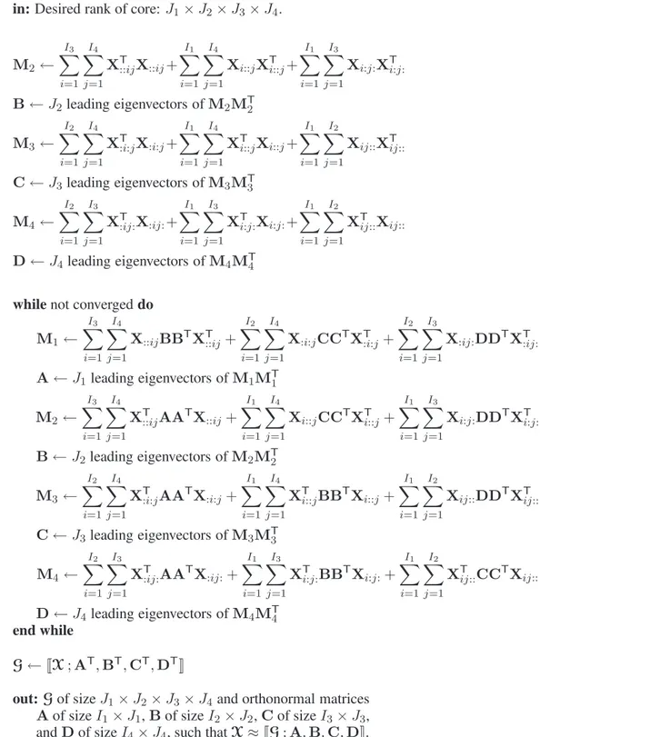
in:Tensor X of sizeI1× I2× I3× I4.
in:Desired rank of core: J1× J2× J3× J4.
D← random matrix of size I4× J4 – normalize columns to unit length
whilenot converged do – main loop
M14← I2 X i=1 I3 X j=1
X:ij:DDTXT:ij: – slices on modes 2 and 3
A← J1 leading eigenvectors of M14MT 14 M21← I3 X i=1 I4 X j=1
XT::ijAATX::ij – slices on modes 3 and 4
B← J2leading eigenvectors of M21MT 21 M32← I1 X i=1 I4 X j=1
XTi::jBBTXi::j – slices on modes 1 and 4
C← J3leading eigenvectors of M32MT 32 M43← I1 X i=1 I2 X j=1
XTij::CCTXij:: – slices on modes 1 and 2
D← J4leading eigenvectors of M43MT
43
end while
G← JX ; AT, BT, CT, DTK
out: Gof sizeJ1× J2× J3× J4 and orthonormal matrices
A of sizeI1× J1, B of sizeI2× J2, C of sizeI3× J3,
and D of sizeI4× J4, such that X≈ JG ; A, B, C, DK.
into RAM. In Figure 5, the matrix C is is filled with random numbers from the uniform distribution over [0, 1] and then the columns are normalized.
Note that HO-SVD calculates each matrix from X alone, whereas HOOI calculates each matrix from X and all of the other matrices. SP lies between HO-SVD and HOOI, in that it calculates each matrix from X and one other matrix.
In the main loop, the input tensor X is processed one slice at a time, again to avoid bringing the whole tensor into RAM. Before entering the main loop, the first step is to calculate the slices and store each slice in a file. MP requires this same first step. The MAT-LAB source code for MP, given in the Appendix, shows how we calculate the slices of X without bringing all of X into RAM.
Our approach to constructing the slice files as-sumes that the input tensor is given in a sparse rep-resentation, in which each nonzero element of the tensor is described by one line in a file. The descrip-tion consists of the indices that specify the locadescrip-tion of the nonzero element, followed by the value of the nonzero element. For example, the elementxijk of
a third-order tensor X is described ashi, j, k, xijki.
To calculate then-mode slices, we first sort the in-put tensor file by moden. For example, we generate two-mode slices by sorting onj, the second column of the input file. This puts all of the elements of an n-mode slice together consecutively in the file. Af-ter sorting on mode n, we can read the sorted file one slice at a time, writing each moden slice to its own unique file.
To sort the input file, we use the Unix sort com-mand. This command allows the user to specify the amount of RAM used by the sort buffer. In the fol-lowing experiments, we arbitrarily set the buffer to 4 GiB, half the available RAM. (For Windows, the Unix sort command is included in Cygwin.)
The main loop terminates after a maximum num-ber of iterations or when the core stops growing, whichever comes first. The growth of the core is measured as follows: ∆G(t) = 1 − G (t−1) F G (t) F (11)
In this equation, G(t) is the core after the t-th iter-ation. We set the threshold for∆G(t) at 10−4 and
we set the maximum number of iterations at50. The main loop usually terminated after half a dozen iter-ations or fewer, with∆G(t) less than 10−4.
SP uses ∆G(t) as a proxy for ∆fit(t), to avoid
bringing X into RAM. With each iteration, as the estimates for the matrices improve, the core captures more of the variation in X, resulting in growth of the core. It is not necessary to bring X into RAM in or-der to calculate G(t); we can calculate G(t)one slice at a time, as given in the Appendix.
For more information about SP, see Wang and Ahuja (2005). Wang et al. (2005) introduced another low RAM algorithm for higher-order tensors, based on blocks instead of slices.
4.4 Multislice Projection
Figure 7 presents the MP algorithm for third-order tensors. The MP algorithm generalizes to arbitrary order. Figure 8 shows MP for fourth-order tensors.
The basic structure of MP is taken from SP, but MP takes three ideas from HOOI: (1) use HO-SVD to initialize, instead of random initialization, (2) use fit to determine convergence, instead of using the growth of the core, (3) use all of the other matri-ces to calculate a given matrix, instead of using only one other matrix. Like SP, MP begins by calculating all of the slices of the input tensor and storing each slice in a file. See the Appendix for details.
We call the initialization pseudo HO-SVD initial-ization, because it is not exactly HO-SVD, as can be seen by comparing the initialization in Figure 3 with the initialization in Figure 7. Note that X(2) in Fig-ure 3 is of sizeI2× (I1I3), whereas M2in Figure 7
is of size I2 × I2, which is usually much smaller.
HO-SVD brings the whole tensor into RAM, but pseudo HO-SVD processes one slice at a time.
The main loop terminates when the change in fit drops below a threshold or when the number of it-erations reaches a maximum, whichever comes first. We calculate the fit one slice at a time, as given in the Appendix; it is not necessary to bring the whole input tensor into RAM in order to calculate the fit. We set the threshold for∆fit(t) at 10−4 and we set
the maximum number of iterations at50. The main loop usually terminated after half a dozen iterations or fewer, with∆fit(t) less than 10−4.
The most significant difference between SP and MP is that MP uses all of the other matrices to cal-culate a given matrix. For example, M13in Figure 5
is based on X and C, whereas the corresponding M1
in Figure 7 is based on X, B, and C. In this respect, MP is like HOOI, as we can see with the correspond-ing U in Figure 3. By sliccorrespond-ing on two modes, instead of only one, we improve the fit of the tensor, as we shall see in the next section.
in:Tensor X of sizeI1× I2× I3.
in:Desired rank of core: J1× J2× J3.
M2 ← I1 X i=1 Xi::XTi::+ I3 X i=1
XT::iX::i – pseudo HO-SVD initialization
B← J2leading eigenvectors of M2MT2 M3 ← I1 X i=1 XT i::Xi::+ I2 X i=1 XT :i:X:i: C← J3leading eigenvectors of M3MT 3
whilenot converged do – main loop
M1← I3 X i=1 X::iBBTXT::i+ I2 X i=1
X:i:CCTXT:i: – slices on modes 2 and 3
A← J1 leading eigenvectors of M1MT 1 M2← I3 X i=1 XT::iAATX::i+ I1 X i=1
Xi::CCTXTi:: – slices on modes 1 and 3
B← J2leading eigenvectors of M2MT2 M3 ← I2 X i=1 XT :i:AATX:i:+ I1 X i=1 XT
i::BBTXi:: – slices on modes 1 and 2
C← J3leading eigenvectors of M3MT
3
end while
G← JX ; AT, BT, CTK
out: Gof sizeJ1× J2× J3and orthonormal matrices A of
sizeI1× J1, B of sizeI2× J2, and C of sizeI3× J3,
such that X≈ JG ; A, B, CK.
Figure 7: Multislice Projection for third-order tensors. MATLAB source code for this algorithm is provided in the Appendix.
in:Tensor X of sizeI1× I2× I3× I4.
in:Desired rank of core: J1× J2× J3× J4.
M2 ← I3 X i=1 I4 X j=1 XT::ijX::ij+ I1 X i=1 I4 X j=1 Xi::jXTi::j+ I1 X i=1 I3 X j=1 Xi:j:XTi:j: B← J2leading eigenvectors of M2MT 2 M3 ← I2 X i=1 I4 X j=1 XT :i:jX:i:j+ I1 X i=1 I4 X j=1 XT i::jXi::j+ I1 X i=1 I2 X j=1 Xij::XT ij:: C← J3leading eigenvectors of M3MT 3 M4 ← I2 X i=1 I3 X j=1 XT:ij:X:ij:+ I1 X i=1 I3 X j=1 XTi:j:Xi:j:+ I1 X i=1 I2 X j=1 XTij::Xij:: D← J4leading eigenvectors of M4MT 4
whilenot converged do
M1← I3 X i=1 I4 X j=1 X::ijBBTXT ::ij+ I2 X i=1 I4 X j=1 X:i:jCCTXT :i:j+ I2 X i=1 I3 X j=1 X:ij:DDTXT :ij: A← J1 leading eigenvectors of M1MT 1 M2 ← I3 X i=1 I4 X j=1 XT::ijAATX::ij+ I1 X i=1 I4 X j=1 Xi::jCCTXTi::j+ I1 X i=1 I3 X j=1 Xi:j:DDTXTi:j: B← J2leading eigenvectors of M2MT 2 M3 ← I2 X i=1 I4 X j=1 XT :i:jAATX:i:j+ I1 X i=1 I4 X j=1 XT i::jBBTXi::j + I1 X i=1 I2 X j=1 Xij::DDTXTij :: C← J3leading eigenvectors of M3MT 3 M4 ← I2 X i=1 I3 X j=1 XT:ij:AATX:ij:+ I1 X i=1 I3 X j=1 XTi:j:BBTXi:j:+ I1 X i=1 I2 X j=1 XTij::CCTXij:: D← J4leading eigenvectors of M4MT 4 end while G← JX ; AT, BT, CT, DTK
out: Gof sizeJ1× J2× J3× J4 and orthonormal matrices
A of sizeI1× J1, B of sizeI2× J2, C of sizeI3× J3,
and D of sizeI4× J4, such that X≈ JG ; A, B, C, DK.
5 Experiments
This section presents the four groups of experiments. The hardware for these experiments was a computer with two dual-core AMD Opteron 64 processors, 8 GiB of RAM, and a 16 GiB swap file. The software was 64 bit Suse Linux 10.0, MATLAB R2007a, and MATLAB Tensor Toolbox Version 2.2 (Bader and Kolda, 2007b). The algorithms only used one of the four cores; we did not attempt to perform allel processing, although SP and MP could be par-allelized readily.
The input files are plain text files with one line for each nonzero value in the tensor. Each line consists of integers that give the location of the nonzero value in the tensor, followed by a single real number that gives the nonzero value itself. The input files are in text format, rather than binary format, in order to facilitate sorting the files.
The output files are binary MATLAB files, con-taining the tensor decompositions of the input files. The four algorithms generate tensor decompositions that are numerically different but structurally identi-cal. That is, the numerical values are different, but, for a given input tensor, the four algorithms generate core tensors and matrices of the same size. There-fore the output file size does not depend on which algorithm was used.
5.1 Varying Tensor Sizes
The goal of this group of experiments was to eval-uate the four algorithms on increasingly larger ten-sors, to discover how their performance scales with size. HO-SVD and HOOI assume that the input ten-sor fits in RAM, whereas SP and MP assume that the input tensor file must be read in blocks. We ex-pected that HO-SVD and HOOI would eventually run out of RAM, but we could not predict precisely how the four algorithms would scale, in terms of fit, time, and space.
Table 1 summarizes the input test tensors for the first group of experiments. The test tensors are ran-dom sparse third-order tensors, varying in size from 2503 to20003. The number of nonzeros in the
ten-sors varies from 1.6 million to 800 million. The nonzero values are random samples from a uniform distribution between zero and one.
Table 2 shows the results of the first group of ex-periments. HO-SVD and HOOI were only able to process the first four tensors, with sizes from2503to
10003. The10003tensor required almost 16 GiB of RAM. The next tensor,12503, required more RAM
than was available (24 GiB; 8 GiB of actual RAM
plus a 16 GiB swap file). On the other hand, SP and MP were able to process all eight tensors, up to20003. Larger tensors are possible with SP and
MP; the limiting factor becomes run time, rather than available RAM.
Figure 9 shows the fit of the four algorithms. HOOI has the best fit, followed by MP, then SP, and finally HO-SVD. The curves for HO-SVD and HOOI stop at 100 million nonzeros (the10003 ten-sor), but it seems likely that the same trend would continue, if sufficient RAM were available to apply HO-SVD and HOOI to the larger tensors.
The fit is somewhat low, at about 4%, due to the difficulty of fitting a random tensor with a core size that is 0.1% of the size of the input tensor. However, we are interested in the relative ranking of the four algorithms, rather than the absolute fit. The results in Section 5.4 show that the ranking we see here, in Figure 9, is predictive of the relative performance on a real (nonrandom) task.
Figure 10 shows the RAM use of the algorithms. As we can see in Table 2, there are two components to the RAM use of SP and MP, the RAM used by
sort and the RAM used by MATLAB. We arbitrarily
set the sorting buffer to 4 GiB, which sets an upper bound on the RAM used by sort. A machine with less RAM could use a smaller sorting buffer. We have not experimented with the buffer size, but we expect that the buffer could be made much smaller, with only a slight increase in run time. The growth of the MATLAB component of RAM use of SP and MP is slow, especially in comparison to HO-SVD and HOOI.
Figure 11 gives the run time. For the smallest ten-sors, SP and MP take longer to run than HO-SVD and HOOI, because SP and MP make more use of files and less use of RAM. With a tensor size of 10003, both HO-SVD and HOOI use up the
avail-able hardware RAM (8 GiB) and need to use the vir-tual RAM (the 16 GiB swap file), which explains the sudden upward surge in Figure 11 at 100 million nonzeros. In general, the run time of SP and MP is competitive with HO-SVD and HOOI.
The results show that SP and MP can handle much larger tensors than HO-SVD and HOOI (800 million nonzeros versus 100 million nonzeros), with only a small penalty in run time for smaller tensors. How-ever, HOOI yields a better fit than MP. If fit is impor-tant, we recommend HOOI for smaller tensors and MP for larger tensors. If speed is more important, we recommend HO-SVD for smaller tensors and SP for larger tensors.
Input tensor size Core size Density Nonzeros Input file Output file
(I1× I2× I3) (J1× J2× J3) (% Nonzero) (Millions) (GiB) (MiB)
250 × 250 × 250 25 × 25 × 25 10 1.6 0.03 0.3 500 × 500 × 500 50 × 50 × 50 10 12.5 0.24 1.5 750 × 750 × 750 75 × 75 × 75 10 42.2 0.81 4.3 1000 × 1000 × 1000 100 × 100 × 100 10 100.0 1.93 9.5 1250 × 1250 × 1250 125 × 125 × 125 10 195.3 3.88 17.7 1500 × 1500 × 1500 150 × 150 × 150 10 337.5 6.85 29.7 1750 × 1750 × 1750 175 × 175 × 175 10 535.9 11.03 46.0 2000 × 2000 × 2000 200 × 200 × 200 10 800.0 16.64 67.4
Table 1: Random sparse third-order tensors of varying size.
Algorithm Tensor Nonzeros Fit Run time Matlab RAM Sort RAM Total RAM
(Millions) (%) (HH:MM:SS) (GiB) (GiB) (GiB)
HO-SVD 2503 1.6 3.890 00:00:24 0.21 0.00 0.21 HO-SVD 5003 12.5 3.883 00:03:44 1.96 0.00 1.96 HO-SVD 7503 42.2 3.880 00:14:42 6.61 0.00 6.61 HO-SVD 10003 100.0 3.880 01:10:13 15.66 0.00 15.66 HOOI 2503 1.6 4.053 00:01:06 0.26 0.00 0.26 HOOI 5003 12.5 3.982 00:09:52 1.98 0.00 1.98 HOOI 7503 42.2 3.955 00:42:45 6.65 0.00 6.65 HOOI 10003 100.0 3.942 04:01:36 15.74 0.00 15.74 SP 2503 1.6 3.934 00:01:21 0.01 1.41 1.42 SP 5003 12.5 3.906 00:10:21 0.02 4.00 4.03 SP 7503 42.2 3.896 00:34:39 0.06 4.00 4.06 SP 10003 100.0 3.893 01:43:20 0.11 4.00 4.12 SP 12503 195.3 3.890 03:16:32 0.21 4.00 4.22 SP 15003 337.5 3.888 06:01:47 0.33 4.00 4.33 SP 17503 535.9 3.886 09:58:36 0.54 4.00 4.54 SP 20003 800.0 3.885 15:35:21 0.78 4.00 4.79 MP 2503 1.6 3.979 00:01:45 0.01 1.41 1.42 MP 5003 12.5 3.930 00:13:55 0.03 4.00 4.03 MP 7503 42.2 3.914 00:51:33 0.06 4.00 4.07 MP 10003 100.0 3.907 02:21:30 0.12 4.00 4.12 MP 12503 195.3 3.902 05:05:11 0.22 4.00 4.23 MP 15003 337.5 3.899 09:28:49 0.37 4.00 4.37 MP 17503 535.9 3.896 16:14:01 0.56 4.00 4.56 MP 20003 800.0 3.894 25:43:17 0.81 4.00 4.82
1 10 100 1,000 3.86% 3.88% 3.90% 3.92% 3.94% 3.96% 3.98% 4.00% 4.02% 4.04% 4.06% HOOI MP SP HO-SVD
Nonzeros (millions)
F
it
(
p
e
rc
e
n
t)
Figure 9: The fit of the four algorithms as a function of the number of nonzeros.
1 10 100 1,000 0.1 1.0 10.0 100.0 HOOI MP SP HO-SVD
Nonzeros (millions)
T
o
ta
l
R
A
M
(
G
iB
)
Figure 10: The RAM use of the four algorithms as a function of the number of nonzeros. Note that the size of the sorting buffer for SP and MP was arbitrarily set to 4 GiB.
1 10 100 1,000 10 100 1,000 10,000 100,000 HOOI MP SP HO-SVD
Nonzeros (millions)
T
im
e
(
s
e
c
o
n
d
s
)
Figure 11: The run time of the four algorithms as a function of the number of nonzeros.
5.2 Varying Core Size Ratios
SP is somewhat different from the other three algo-rithms, in that it has a kind of asymmetry. Compare M13 in Figure 5 with M1 in Figure 7. We could have used B instead of C, to calculate A in Fig-ure 5, but we arbitrarily chose C. We hypothesized that this asymmetry would make SP sensitive to vari-ation in the ratios of the core sizes.
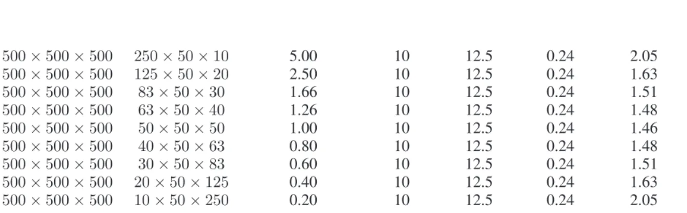
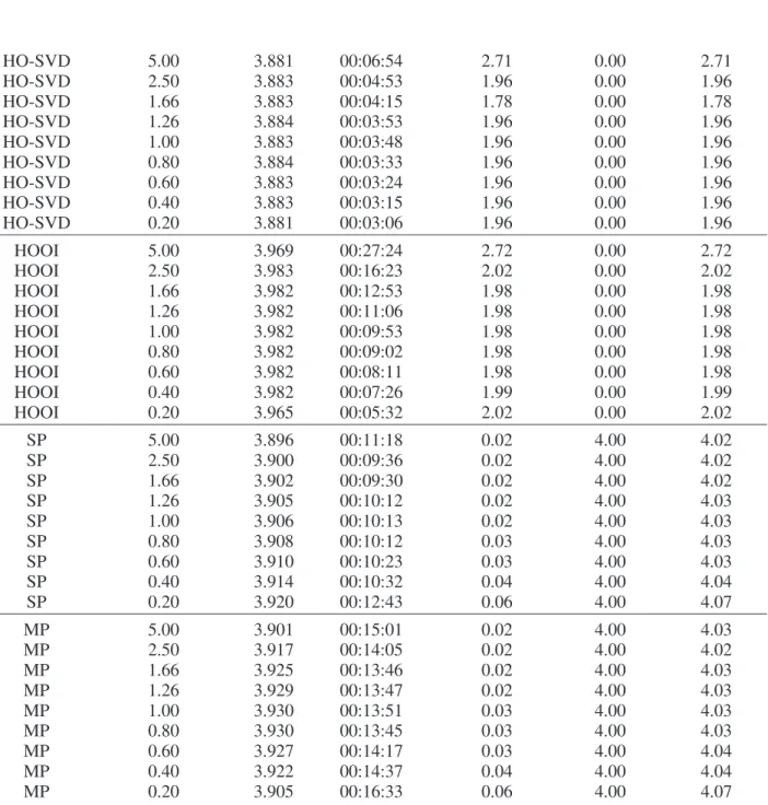
In this group of experiments, we vary the ratios between the sizes of the core in each mode, as listed in Table 3. The effect of the ratio on the performance is shown in Table 4. Figure 12 illustrates the effect of the ratio on the fit. It is clear from the figure that SP is asymmetrical, whereas HO-SVD, HOOI, and MP are symmetrical.
This asymmetry of SP might be viewed as a flaw, and thus a reason for preferring MP over SP, but it could also be seen as an advantage for SP. In the case where the ratio is 0.2, SP has a better fit than MP. This suggests that we might use SP instead of MP when the ratios between the sizes of the core in each mode are highly skewed; however, we must be careful to make sure that SP processes the matrices in the optimal order for the given core sizes.
Note that the relative ranking of the fit of the four algorithms is the same as in the previous group
of experiments (best fit to worst: HOOI, MP, SP, HO-SVD), except in the case of extreme skew. Thus Figure 12 shows the robustness of the relative rank-ing.
5.3 Fourth-Order Tensors
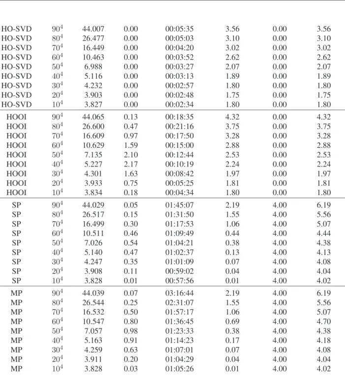
This group of experiments demonstrates that the pre-vious observations regarding the relative ranking of the fit also apply to fourth-order tensors. The exper-iments also investigate the effect of varying the size of the core, with a fixed input tensor size.
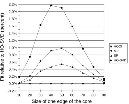
Table 5 lists the core sizes that we investigated. The effect of the core sizes on the performance is shown in Table 6. Figure 13 shows the impact of core size on fit.
The fit varies from about 4% with a core of 104 to about 44% with a core of904. To make the
dif-ferences among the algorithms clearer, we normal-ized the fit by using HO-SVD as a baseline. The fit relative to HO-SVD is defined as the percentage improvement in the fit of the given algorithm, com-pared to the fit of HO-SVD.
Figure 13 shows that the differences among the four algorithms are largest when the core is about 504; that is, the size of one mode of the core (50) is
Input tensor size Core size Ratio Density Nonzeros Input file Output file (I1× I2× I3) (J1× J2× J3) (J1/J2=J2/J3) (%) (Millions) (GiB) (MiB)
500 × 500 × 500 250 × 50 × 10 5.00 10 12.5 0.24 2.05 500 × 500 × 500 125 × 50 × 20 2.50 10 12.5 0.24 1.63 500 × 500 × 500 83 × 50 × 30 1.66 10 12.5 0.24 1.51 500 × 500 × 500 63 × 50 × 40 1.26 10 12.5 0.24 1.48 500 × 500 × 500 50 × 50 × 50 1.00 10 12.5 0.24 1.46 500 × 500 × 500 40 × 50 × 63 0.80 10 12.5 0.24 1.48 500 × 500 × 500 30 × 50 × 83 0.60 10 12.5 0.24 1.51 500 × 500 × 500 20 × 50 × 125 0.40 10 12.5 0.24 1.63 500 × 500 × 500 10 × 50 × 250 0.20 10 12.5 0.24 2.05
Table 3: Random sparse third-order tensors with varying ratios between the sizes of the core in each mode.
0.1 1 10 3.88% 3.89% 3.90% 3.91% 3.92% 3.93% 3.94% 3.95% 3.96% 3.97% 3.98% 3.99% HOOI MP SP HO-SVD
Ratio of edge sizes of the core
F
it
(
p
e
rc
e
n
t)
Figure 12: The fit of the four algorithms as a function of the ratios between the sizes of the core in each mode.
Algorithm Ratio Fit Run time Matlab RAM Sort RAM Total RAM
(J1/J2 = J2/J3) (%) (HH:MM:SS) (GiB) (GiB) (GiB)
HO-SVD 5.00 3.881 00:06:54 2.71 0.00 2.71 HO-SVD 2.50 3.883 00:04:53 1.96 0.00 1.96 HO-SVD 1.66 3.883 00:04:15 1.78 0.00 1.78 HO-SVD 1.26 3.884 00:03:53 1.96 0.00 1.96 HO-SVD 1.00 3.883 00:03:48 1.96 0.00 1.96 HO-SVD 0.80 3.884 00:03:33 1.96 0.00 1.96 HO-SVD 0.60 3.883 00:03:24 1.96 0.00 1.96 HO-SVD 0.40 3.883 00:03:15 1.96 0.00 1.96 HO-SVD 0.20 3.881 00:03:06 1.96 0.00 1.96 HOOI 5.00 3.969 00:27:24 2.72 0.00 2.72 HOOI 2.50 3.983 00:16:23 2.02 0.00 2.02 HOOI 1.66 3.982 00:12:53 1.98 0.00 1.98 HOOI 1.26 3.982 00:11:06 1.98 0.00 1.98 HOOI 1.00 3.982 00:09:53 1.98 0.00 1.98 HOOI 0.80 3.982 00:09:02 1.98 0.00 1.98 HOOI 0.60 3.982 00:08:11 1.98 0.00 1.98 HOOI 0.40 3.982 00:07:26 1.99 0.00 1.99 HOOI 0.20 3.965 00:05:32 2.02 0.00 2.02 SP 5.00 3.896 00:11:18 0.02 4.00 4.02 SP 2.50 3.900 00:09:36 0.02 4.00 4.02 SP 1.66 3.902 00:09:30 0.02 4.00 4.02 SP 1.26 3.905 00:10:12 0.02 4.00 4.03 SP 1.00 3.906 00:10:13 0.02 4.00 4.03 SP 0.80 3.908 00:10:12 0.03 4.00 4.03 SP 0.60 3.910 00:10:23 0.03 4.00 4.03 SP 0.40 3.914 00:10:32 0.04 4.00 4.04 SP 0.20 3.920 00:12:43 0.06 4.00 4.07 MP 5.00 3.901 00:15:01 0.02 4.00 4.03 MP 2.50 3.917 00:14:05 0.02 4.00 4.02 MP 1.66 3.925 00:13:46 0.02 4.00 4.03 MP 1.26 3.929 00:13:47 0.02 4.00 4.03 MP 1.00 3.930 00:13:51 0.03 4.00 4.03 MP 0.80 3.930 00:13:45 0.03 4.00 4.03 MP 0.60 3.927 00:14:17 0.03 4.00 4.04 MP 0.40 3.922 00:14:37 0.04 4.00 4.04 MP 0.20 3.905 00:16:33 0.06 4.00 4.07
Input tensor size Core size Density Nonzeros Input file Output file
(I1× I2× I3× I4) (J1× J2× J3× J4) (%) (Millions) (MiB) (MiB)
1004 904 10 10 197.13 480.68 1004 804 10 10 197.13 300.16 1004 704 10 10 197.13 176.02 1004 604 10 10 197.13 95.08 1004 504 10 10 197.13 45.91 1004 404 10 10 197.13 18.86 1004 304 10 10 197.13 6.02 1004 204 10 10 197.13 1.23 1004 104 10 10 197.13 0.10
Table 5: Random sparse fourth-order tensors with varying core sizes.
10 20 30 40 50 60 70 80 90 -0.2% 0.0% 0.2% 0.4% 0.6% 0.8% 1.0% 1.2% 1.4% 1.6% 1.8% 2.0% 2.2% HOOI MP SP HO-SVD
Size of one edge of the core
F
it
r
e
la
ti
v
e
t
o
H
O
-S
V
D
(
p
e
rc
e
n
t)
Algorithm Core Size Fit Relative fit Run time Matlab RAM Sort RAM Total RAM
(%) (%) (HH:MM:SS) (GiB) (GiB) (GiB)
HO-SVD 904 44.007 0.00 00:05:35 3.56 0.00 3.56 HO-SVD 804 26.477 0.00 00:05:03 3.10 0.00 3.10 HO-SVD 704 16.449 0.00 00:04:20 3.02 0.00 3.02 HO-SVD 604 10.463 0.00 00:03:52 2.62 0.00 2.62 HO-SVD 504 6.988 0.00 00:03:27 2.07 0.00 2.07 HO-SVD 404 5.116 0.00 00:03:13 1.89 0.00 1.89 HO-SVD 304 4.232 0.00 00:02:57 1.80 0.00 1.80 HO-SVD 204 3.903 0.00 00:02:48 1.75 0.00 1.75 HO-SVD 104 3.827 0.00 00:02:34 1.80 0.00 1.80 HOOI 904 44.065 0.13 00:18:35 4.32 0.00 4.32 HOOI 804 26.600 0.47 00:21:16 3.75 0.00 3.75 HOOI 704 16.609 0.97 00:17:50 3.28 0.00 3.28 HOOI 604 10.629 1.59 00:15:00 2.88 0.00 2.88 HOOI 504 7.135 2.10 00:12:44 2.53 0.00 2.53 HOOI 404 5.227 2.17 00:10:19 2.24 0.00 2.24 HOOI 304 4.301 1.63 00:08:42 1.97 0.00 1.97 HOOI 204 3.933 0.75 00:05:25 1.81 0.00 1.81 HOOI 104 3.834 0.18 00:04:34 1.80 0.00 1.80 SP 904 44.029 0.05 01:45:07 2.19 4.00 6.19 SP 804 26.517 0.15 01:31:50 1.55 4.00 5.56 SP 704 16.499 0.30 01:17:53 1.06 4.00 5.07 SP 604 10.511 0.46 01:09:49 0.44 4.00 4.44 SP 504 7.026 0.54 01:04:21 0.38 4.00 4.38 SP 404 5.140 0.47 01:02:37 0.13 4.00 4.13 SP 304 4.247 0.35 01:01:09 0.07 4.00 4.08 SP 204 3.908 0.11 00:59:02 0.04 4.00 4.04 SP 104 3.828 0.01 00:57:56 0.01 4.00 4.02 MP 904 44.039 0.07 03:16:44 2.19 4.00 6.19 MP 804 26.544 0.25 02:31:07 1.55 4.00 5.56 MP 704 16.532 0.50 01:57:17 1.06 4.00 5.07 MP 604 10.547 0.80 01:36:45 0.69 4.00 4.70 MP 504 7.057 0.98 01:23:33 0.38 4.00 4.38 MP 404 5.163 0.91 01:14:23 0.17 4.00 4.18 MP 304 4.259 0.63 01:07:01 0.07 4.00 4.08 MP 204 3.911 0.20 01:04:29 0.04 4.00 4.04 MP 104 3.828 0.03 01:05:26 0.01 4.00 4.02
Table 6: Performance of the four algorithms with fourth-order tensors and varying core sizes. Relative fit is the percentage increase in fit relative to HO-SVD.
(100). When the core is very small or very large, compared to the input tensor, there is little difference in fit among the algorithms.
The fit follows the same trend here as in the pre-vious two groups of experiments (best to worst: HOOI, MP, SP, HO-SVD), in spite of the switch from third-order tensors to fourth-order tensors. This further confirms the robustness of the results.
Table 6 shows that SP and MP are slow with fourth-order tensors, compared to HO-SVD and HOOI. This is a change from what we observered with third-order tensors, which did not yield such large differences in run time. This is because a fourth-order tensor has many more slices than a third-order tensor with the same number of ele-ments, and each slice is smaller. There is a much larger overhead associated with opening and clos-ing many small files, compared to a few large files. This could be ameliorated by storing several adja-cent slices together in one file, instead of using a separate file for each slice.
Even with third-order tensors, grouping slices to-gether in one file would improve the speed of SP and MP. Ideally, the user would specify the maxi-mum RAM available and SP and MP would group as many slices together as would fit in the available RAM.
5.4 Performance with Real Data
So far, all our experiments have used random ten-sors. Our purpose with this last group of experi-ments is to show that the previous observations ap-ply to nonrandom tensors. In particular, the differ-ences in fit that we have seen so far are somewhat small. It seems possible that the differences might not matter in a real application of tensors. This group of experiments shows that the differences in fit result in differences in performance on a real task. The task we examine here is answering multiple-choice synonym questions from the TOEFL test. This task was first investigated in Landauer and Du-mais (1997). In ongoing work, we are exploring the application of third-order tensors to this task, com-bining ideas from Landauer and Dumais (1997) and Turney (2006).
Table 7 describes the input data and the output tensor decomposition. The first mode of the tensor consists of all of the 391 unique words that occur in the TOEFL questions. The second mode is a set of 849 words from Basic English, which is an artifi-cial language that reduces English to a small, easily learned core vocabulary (Ogden, 1930). The third
mode consists of 1020 patterns that join the words in the first two modes. These patterns were gener-ated using the approach of Turney (2006). The value of an element in the tensor is derived from the fre-quency of the corresponding word pair and pattern in a large corpus.
A TOEFL question consists of a stem word (the target word) and four choice words. The task is to select the choice word that is most similar in mean-ing to the stem word. Our approach is to measure the similarity of two TOEFL words by the average sim-ilarity of their relations to the Basic English words.
Let X be our input tensor. Suppose we wish to measure the similarity of two TOEFL words. Let Xi:: and Xj:: be the slices of X that correspond to the two TOEFL words. Each slice gives the weights for all of the patterns that join the given TOEFL word to all of the Basic English words. Our mea-sure of similarity between the TOEFL words is cal-culated by comparing the two slices.
Table 8 presents the performance of the four algo-rithms. We see that the fit follows the familiar pat-tern: HOOI has the best fit, then MP, next SP, and lastly HO-SVD. Note that MP and SP have similar fits. The final column of the table gives the TOEFL scores for the four algorithms. HOOI has the best TOEFL score, MP and SP have the same score, and HO-SVD has the lowest score. The bottom row of the table gives the TOEFL score for the raw input tensor, without the benefit of any smoothing from the Tucker decomposition. The results validate the previous experiments with random tensors and illus-trate the value of the Tucker decomposition on a real task.
6 Conclusions
The Tucker decomposition has been with us since 1966, but it seems that it has only recently started to become popular. We believe that this is because only recently has computer hardware reached the point where large tensor decompositions are becom-ing feasible.
SVD started to attract interest in the field of in-formation retrieval when it was applied to “prob-lems of reasonable size (1000-2000 document ab-stracts; and 5000-7000 index terms)” (Deerwester et al., 1990). In collaborative filtering, SVD attracted interest when it achieved good results on the Net-flix Prize, a dataset with a sparse matrix of 17,000 movies rated by 500,000 users. In realistic applica-tions, size matters. The MATLAB Tensor Toolbox (Bader and Kolda, 2007a; Bader and Kolda, 2007b)
Input tensor size (I1× I2× I3) 391 × 849 × 1020
Core size (J1× J2× J3) 250 × 250 × 250
Input file (MiB) 345
Output file (MiB) 119
Density (% Nonzero) 5.27
Nonzeros (Millions) 18
Table 7: Description of the input data and the output decomposition.
Algorithm Fit Relative fit Run time Matlab RAM Sort RAM Total RAM TOEFL
(%) (%) (HH:MM:SS) (GiB) (GiB) (GiB) (%)
HO-SVD 21.716 0.00 00:10:28 5.29 0.00 5.29 80.00
HOOI 22.597 4.05 00:56:08 5.77 0.00 5.77 83.75
SP 22.321 2.78 00:30:02 0.33 4.00 4.33 81.25
MP 22.371 3.01 00:43:52 0.33 4.00 4.34 81.25
Raw tensor - - - 67.50
Table 8: Performance of the four algorithms with actual data. Relative fit is the percentage increase in fit relative to HO-SVD.
has done much to make tensor decompositions more accessible and easier to experiment with, but, as we have seen here, RAM requirements become prob-lematic with tensors larger than10003.
The aim of this paper has been to empirically eval-uate four tensor decompositions, to study their fit and their time and space requirements. Our primary concern was the ability of the algorithms to scale up to large tensors. The implementations of HO-SVD and HOOI, taken from the MATLAB Tensor Tool-box, assumed that the input tensor could fit in RAM, which limited them to tensors of size10003. On the other hand, SP and MP were able to process tensors of size20003, with eight times more elements.
The experiments in Section 5.4 suggest that the differences in fit among the four algorithms corre-spond to differences in performance on real tasks. It seems likely that good fit will be important for many applications; therefore, we recommend HOOI for those tensors that can fit in the available RAM, and MP for larger tensors.
Acknowledgements
Thanks to Brandyn Webb, Tamara Kolda, and Hongcheng Wang for helpful comments. Thanks to Tamara Kolda and Brett Bader for the MATLAB Tensor Toolbox.
References
E. Acar and B. Yener. 2007. Unsupervised multiway data analysis: A literature survey. Technical report, Computer Science Department, Rensselaer Polytech-nic Institute, Troy, NY. http://www.cs.rpi.edu/∼acare/ Acar07 Multiway.pdf.
O. Alter, P.O. Brown, and D. Botstein. 2000. Singular value decomposition for genome-wide expression data processing and modeling. Proceedings of the National
Academy of Sciences, 97(18):10101–10106.
B.W. Bader and T.G. Kolda. 2007a. Efficient MATLAB computations with sparse and factored tensors. SIAM
Journal on Scientific Computing.
B.W. Bader and T.G. Kolda. 2007b. MATLAB Ten-sor Toolbox version 2.2. http://csmr.ca.sandia.gov/ ∼tgkolda/TensorToolbox/.
D. Billsus and M.J. Pazzani. 1998. Learning collabora-tive information filters. Proceedings of the Fifteenth
International Conference on Machine Learning, pages
46–54.
M. Brand. 2002. Incremental singular value decompo-sition of uncertain data with missing values.
Proceed-ings of the 7th European Conference on Computer Vi-sion, pages 707–720.
R. Bro and C.A. Andersson. 1998. Improving the speed of multiway algorithms – Part II: Compres-sion. Chemometrics and Intelligent Laboratory
J.D. Carroll and J.J. Chang. 1970. Analysis of indi-vidual differences in multidimensional scaling via an n-way generalization of “Eckart-Young” decomposi-tion. Psychometrika, 35(3):283–319.
P.A. Chew, B.W. Bader, T.G. Kolda, and A. Abde-lali. 2007. Cross-language information retrieval using PARAFAC2. Proceedings of the 13th ACM SIGKDD
International Conference on Knowledge Discovery and Data Mining, pages 143–152.
L. De Lathauwer, B. De Moor, and J. Vandewalle. 2000a. A multilinear singular value decomposition.
SIAM Journal on Matrix Analysis and Applications,
21:1253–1278.
L. De Lathauwer, B. De Moor, and J. Vandewalle. 2000b. On the best rank-1 and rank-(R1, R2, . . . , RN)
ap-proximation of higher-order tensors. SIAM Journal on
Matrix Analysis and Applications, 21:1324–1342.
S. Deerwester, S.T. Dumais, G.W. Furnas, T.K. Landauer, and R. Harshman. 1990. Indexing by latent semantic analysis. Journal of the American Society for
Informa-tion Science, 41(6):391–407.
D.M. Dunlavy, T.G. Kolda, and W.P. Kegelmeyer. 2006. Multilinear algebra for analyzing data with multiple linkages. Technical Report SAND2006-2079, Sandia National Laboratories, Livermore, CA. http://csmr.ca.sandia.gov/∼tgkolda/pubs/SAND2006-2079.pdf.
R.A. Harshman. 1970. Foundations of the PARAFAC procedure: Models and conditions for an “explana-tory” multi-modal factor analysis. UCLA Working
Pa-pers in Phonetics, 16:1–84.
T.G. Kolda. 2006. Multilinear operators for higher-order decompositions. Technical Report SAND2006-2081, Sandia National Laboratories, Livermore, CA. http://csmr.ca.sandia.gov/∼tgkolda/pubs/SAND2006-2081.pdf.
T.K. Landauer and S.T. Dumais. 1997. A solution to Plato’s problem: The latent semantic analysis theory of acquisition, induction, and representation of knowl-edge. Psychological Review, 104(2):211–240. M.W. Mahoney, M. Maggioni, and P. Drineas. 2006.
Tensor-CUR decompositions for tensor-based data.
Proceedings of the 12th ACM SIGKDD International Conference on Knowledge Discovery and Data Min-ing, pages 327–336.
C.K. Ogden. 1930. Basic English: A general in-troduction with rules and grammar. Kegan Paul, Trench, Trubner and Co., London. http://ogden.basic-english.org/.
H. Sch¨utze. 1998. Automatic word sense discrimination.
Computational Linguistics, 24(1):97–123.
J. Sun, D. Tao, and C. Faloutsos. 2006. Beyond streams and graphs: Dynamic tensor analysis. Proceedings of
the 12th ACM SIGKDD International Conference on Knowledge Discovery and Data Mining, pages 374–
383.
L.R. Tucker. 1966. Some mathematical notes on three-mode factor analysis. Psychometrika, 31(3):279–311. P.D. Turney. 2006. Similarity of semantic relations.
Computational Linguistics, 32(3):379–416.
H. Wang and N. Ahuja. 2005. Rank-R approximation of tensors: Using image-as-matrix representation.
Pro-ceedings of the 2005 IEEE Computer Society Con-ference on Computer Vision and Pattern Recognition (CVPR’05), 2:346–353.
H. Wang, Q. Wu, L. Shi, Y. Yu, and N. Ahuja. 2005. Out-of-core tensor approximation of multi-dimensional matrices of visual data. International Conference on
Computer Graphics and Interactive Techniques, SIG-GRAPH 2005, 24:527–535.
Y. Xu, L. Zhang, and W. Liu. 2006. Cubic analysis of social bookmarking for personalized recommenda-tion. Lecture Notes in Computer Science: Frontiers
of WWW Research and Development – APWeb 2006,
Appendix: MATLAB Source for Multislice Projection
---function fit = multislice(data_dir,sparse_file,tucker_file,I,J)
%MULTISLICE is a low RAM Tucker decomposition %
% Peter Turney % October 26, 2007 %
% Copyright 2007, National Research Council of Canada %
% This program is free software: you can redistribute it and/or modify % it under the terms of the GNU General Public License as published by % the Free Software Foundation, either version 3 of the License, or % (at your option) any later version.
%
% This program is distributed in the hope that it will be useful, % but WITHOUT ANY WARRANTY; without even the implied warranty of % MERCHANTABILITY or FITNESS FOR A PARTICULAR PURPOSE. See the % GNU General Public License for more details.
%
% You should have received a copy of the GNU General Public License % along with this program. If not, see <http://www.gnu.org/licenses/>. %
%% set parameters %
fprintf(’MULTISLICE is running ...\n’); %
maxloops = 50; % maximum number of iterations eigopts.disp = 0; % suppress messages from eigs() minfitchange = 1e-4; % minimum change in fit of tensor %
%% make slices of input data file %
fprintf(’ preparing slices\n’); % mode1_dir = ’slice1’; mode2_dir = ’slice2’; mode3_dir = ’slice3’; % slice(data_dir,sparse_file,mode1_dir,1,I); slice(data_dir,sparse_file,mode2_dir,2,I); slice(data_dir,sparse_file,mode3_dir,3,I); %
%% pseudo HO-SVD initialization % % initialize B % M2 = zeros(I(2),I(2)); for i = 1:I(3) X3_slice = load_slice(data_dir,mode3_dir,i); M2 = M2 + (X3_slice’ * X3_slice); end for i = 1:I(1) X1_slice = load_slice(data_dir,mode1_dir,i); M2 = M2 + (X1_slice * X1_slice’); end [B,D] = eigs(M2*M2’,J(2),’lm’,eigopts); % % initialize C % M3 = zeros(I(3),I(3)); for i = 1:I(1) X1_slice = load_slice(data_dir,mode1_dir,i); M3 = M3 + (X1_slice’ * X1_slice); end for i = 1:I(2) X2_slice = load_slice(data_dir,mode2_dir,i); M3 = M3 + (X2_slice’ * X2_slice); end
[C,D] = eigs(M3*M3’,J(3),’lm’,eigopts); % %% main loop % old_fit = 0; %
fprintf(’ entering main loop of MULTISLICE\n’); %
for loop_num = 1:maxloops % % update A % M1 = zeros(I(1),I(1)); for i = 1:I(2) X2_slice = load_slice(data_dir,mode2_dir,i); M1 = M1 + ((X2_slice * C) * (C’ * X2_slice’)); end for i = 1:I(3) X3_slice = load_slice(data_dir,mode3_dir,i); M1 = M1 + ((X3_slice * B) * (B’ * X3_slice’)); end [A,D] = eigs(M1*M1’,J(1),’lm’,eigopts); % % update B % M2 = zeros(I(2),I(2)); for i = 1:I(3) X3_slice = load_slice(data_dir,mode3_dir,i); M2 = M2 + ((X3_slice’ * A) * (A’ * X3_slice)); end for i = 1:I(1) X1_slice = load_slice(data_dir,mode1_dir,i); M2 = M2 + ((X1_slice * C) * (C’ * X1_slice’)); end [B,D] = eigs(M2*M2’,J(2),’lm’,eigopts); % % update C % M3 = zeros(I(3),I(3)); for i = 1:I(1) X1_slice = load_slice(data_dir,mode1_dir,i); M3 = M3 + ((X1_slice’ * B) * (B’ * X1_slice)); end for i = 1:I(2) X2_slice = load_slice(data_dir,mode2_dir,i); M3 = M3 + ((X2_slice’ * A) * (A’ * X2_slice)); end
[C,D] = eigs(M3*M3’,J(3),’lm’,eigopts); %
% build the core % G = zeros(I(1)*J(2)*J(3),1); G = reshape(G,[I(1) J(2) J(3)]); for i = 1:I(1) X1_slice = load_slice(data_dir,mode1_dir,i); G(i,:,:) = B’ * X1_slice * C; end G = reshape(G,[I(1) (J(2)*J(3))]); G = A’ * G; G = reshape(G,[J(1) J(2) J(3)]); % % measure fit % normX = 0; sqerr = 0; for i = 1:I(1) X1_slice = load_slice(data_dir,mode1_dir,i); X1_approx = reshape(G,[J(1) (J(2)*J(3))]); X1_approx = A(i,:) * X1_approx;
X1_approx = reshape(X1_approx,[J(2) J(3)]); X1_approx = B * X1_approx * C’;