Asynchronous receivers in narrowband packet radio applications

Asynchronous Receivers in Narrowband Packet Radio Applications

by

Submitted to the Department of Electrical Engineering and Computer Science in Partial Fulfillment of the Requirements for the Degrees of

Bachelor of Science in Electrical Science and Engineering

and Master of Engineering in Electrical Engineering and Computer Science at the Massachusetts Institute of Technology

May 23, 1997

Copyright 1997 Amit G. Bagchi. All rights reserved.

The author hereby grants to M.I.T. permission to reproduce and distribute publicly paper and electronic copies of this thesis

and to grant others the right to do so.

Author . _

Department of Electrical ngineering and Computer Science May 23, 1997

Certified by. __.

Amos Lapidoth Thesidutirvisor Accepted by

Chairman partment Committee duate Theses

" " ,V/. ,

Asynchronous Receivers in Narrowband Packet Radio Applications:

Personal Access Communications System (PACS) and the U.S. Asynchronous Band

by

Amit G. Bagchi Submitted to the

Department of Electrical Engineering and Computer Science May 23, 1997

In Partial Fulfillment of the Requirements for the Degree of Bachelor of Science in Electrical Science and Engineering

and Master of Engineering in Electrical Engineering and Computer Science

ABSTRACT

A burst coherent receiver capable of operating efficiently in packet radio applications is studied. Rules for use of the U.S. Asynchronous spectrum are discussed, with attention to their implications for receiver design. An existing design by Bell Communications Research is reviewed in the context of packet radio applications and problems with this design that lead to low spectral efficiency and low throughput are noted. Two major problems are found to be excessive synchronization overhead and excessive processing latency. A technique for reducing latency by variable rate processing is described in detail, with analysis of achievable reductions provided. Methods for reducing synchronization overhead are proposed, and a simulation environment for evaluating their performance is presented. Finally, limited simulation results are provided for initial performance estimates.

Thesis Supervisor: Amos Lapidoth

Table of Contents

1. ACKNOWLEDGEMENT ... 4

2. INTRODUCTION ... 5

2.1 M OTIVATION... ... ... ... 5

2.2 U.S. SPECTRUM FOR ASYNCHRONOUS USE ... 5

2.3 PERSONAL ACCESS COMMUNICATIONS SYSTEM (PACS)... ... 6

2.4 PACKET D ATA A PPLICATIONS... ... ... 6

3. U.S. ASYNCHRONOUS SPECTRUM RULES ... 7

4. PACS DESIGN AND THE ASYNCHRONOUS SPECTRUM ... 8

4.1 CHANNEL M ODEL... . ... . ... ... ... 9

4.2 M ODULATION... . . ... ... 9

4.3 ERROR CHECK CODING ... 10

4.4 BURST SIZE / SYMBOL RATE ... 10

4.5 COHERENT DEMODULATION ... 11

5. PROBLEMS OF THE EXISTING PACS RECEIVER... 12

5.1 TRANSMISSION OVERHEAD AND MINIMUM PACKET SIZE ... 12

5.2 DEMODULATION / DECODE LATENCY AND TERMINAL RESPONSE TIME... .... 14

6. NEW RECEIVER TECHNIQUES ... 15

6.1 MEDIA ACCESS CONTROL PERSPECTIVE... 15

6.2 REDUCING LATENCY... ... ... ... 18

6.2.1 Variable Rate Processing ... 18

6.2.2 Required Buffering... ... ... 23

6.3 REDUCING SYNCHRONIZATION OVERHEAD ... ... 25

6.3.1 Correlation Position in Burst ... ... 26

6.3.2 Parallelism -Multiple Staggered Receive Windows ... ... 27

6.3.3 Half Burst Demodulator... ... ... 27

7. ANALYSIS OF CHANNEL ESTIMATES AND CARRIER RECOVERY ... 28

7.1 SYMBOL TIMING QUALITY INDEX (QI) AND FREQUENCY OFFSET ESTIMATION ... 29

7.2 CARRIER RECOVERY SECOND ORDER LOOP ... 37

8. WHOLE BURST RECEIVER WITH BACKWARD BUFFERING... ... 44

9. HALF BURST RECEIVER ... 45

10. HIGHLY PARALLEL RECEIVER ... 50

11. SIMULATION AND EVALUATION ... 54

11.1 FRONT END ASSUMPTIONS ... 55

11.2 MODELING CHANNEL IMPAIRMENT... 57

11.3 MODELING QUANTIZATION ERROR... 58

11.4 MODELING IMPLEMENTATION LATENCY AND SYNCHRONIZATION ... 59

11.5 MEASURING PERFORMANCE _{... 61}

12.1 TESTING PLAN... 64

12.2 TEST RESULTS ... 67

13. CONCLUSION ... 72

13.1 FUTURE VERIFICATION AND QUANTITATIVE ESTIMATES ... ... 72

13.2 RECOM MENDATIONS FOR PROTOCOL STUDY ... 73

13.3 SUMMARY ... 74

Table of Figures

FIGURE 4-1 DIFFERENTIAL (LEFT) AND ABSOLUTE (RIGHT) PHASE CONSTELLATIONS FOR r/4 SHIFT DQPSK 10

FIGURE 5-1 RECEIVER PIPELINE STAGES ... ... 13

FIGURE 5-2 OVERHEAD REQUIREMENTS OF CURRENT DESIGN ... ... 14

FIGURE 6-1 POLLING ACCESS PIGGYBACKING TRANSMISSIONS ... 17

FIGURE 6-2 EXISTING DESIGN (LEFT), AND VARIABLE PROCESSING IMPROVEMENT (RIGHT) ... 20

FIGURE 6-3 LATENCIES WITH VARIABLE RATE PROCESSING ... ... 22

FIGURE 6-4 LATENCY AS A FUNCTION OF VARIABLE PROCESSING RATE ... 23

FIGURE 6-5 OVERHEAD REQUIREMENTS OF REDUCED LATENCY RECEIVER... 26

FIGURE 7-1 ZERO ISI PULSE SHAPES ... ... 30

FIGURE 7-2 BANDPASS TO PHASE CONVERSION... 31

FIGURE 7-3 QI AND FREQUENCY OFFSET COMPUTATION ... ... 32

FIGURE 7-4 QI AS A FUNCTION OF SAMPLING OFFSET IN THE ABSENCE OF NOISE, (LONG ACCUMULATION)... 33

FIGURE 7-5 EMPIRICAL CDFS AT SEVERAL SNRs ... ... 37

FIGURE 7-6 CARRIER RECOVERY SECOND ORDER LOOP ... ... 40

FIGURE 7-7 POLE AND ZERO LOCATIONS FOR CARRIER RECOVERY LOOP ... 41

FIGURE 7-8 STEP AND RAMP RESPONSES FOR CARRIER RECOVERY LOOP... ... 42

FIGURE 9-1 LATENCY OF HALF BURST RECEIVER ... ... 48

FIGURE 9-2 SYNCHRONIZATION TIMING FOR HALF BURST RECEIVER ... ... 49

FIGURE 12-1 PULSE SHAPED ABSOLUTE PHASE CONSTELLATION ... 65

FIGURE 12-2 PRE-TRANSMISSION CHANNEL IMPAIRMENT ... ... 66

FIGURE 12-3 ADDITIVE PHASOR NOISE, CHANNEL IMPAIRMENT ... ... 67

1. Acknowledgement

This work would not have been possible without the valuable assistance of Dr. Robert Ziegler, Director of the Wireless Enterprise Systems Group at Bell

Communications Research, Inc. (Bellcore). His initial development of MATLAB

simulations for the PACS demodulator, as well has his comments and suggestions are the foundation for this work. Bellcore Research Scientist Gregory Pollini was instrumental in formulating the latency of the PACS receiver, and my collaboration with him is included here. All of the members of the Wireless Enterprise Systems Group and the Wireless Techniques and Technologies Group, have been very supportive in the course of this work. Finally, Massachusetts Institute of Technology Professor Amos Lapidoth, provided guidance as my thesis advisor.

2. Introduction

2.1 Motivation

In recent years the U.S. has experienced a fast growing demand for tetherless data capability, wireless local area networks, and mobile networking capability. This, coupled with the recent allocation of U.S. spectrum for such use, has led many to develop these systems. However, relatively high bit error rates are tolerated in developing the required physical layer hardware. The motivation for exploring burst coherent receivers for these applications, is the lower bit error rates that they provide. Bell Communications Research has designed a burst coherent receiver suitable for circuit switched telephony with the Personal Access Communications System standard. However, the higher processing latency associated with this receiver renders it inefficient in packet switched applications. It is the author's intention to design a coherent receiver suitable for packet radio

applications with relatively low bit error rates.

2.2

U.S. Spectrum for Asynchronous Use

In order to better understand the design requirements for the desired receiver, the target spectrum must be discussed. The United States Federal Communications

Commission (FCC) has allocated the electromagnetic spectrum between 1850 and 1990 MHz for the delivery of "Personal Communications Services." It is referred to as the Emerging Technologies Spectrum for Broadband PCS, and it is subdivided into licensed and unlicensed bands. In the licensed band, providers have purchased the rights to spectrum at auction, whereas in the unlicensed band, any device may operate that conforms to FCC specified usage rules. The unlicensed band is further subdivided into

Isochronous and Asynchronous bands. The FCC Isochronous Band rules enable

telephony applications such as wireless PBXs, while the Asynchronous rules enable packet radio applications such as wireless LANs. It is the availability of the Unlicensed

Asynchronous Spectrum between 1910 and 1930 MHz that motivates the development of asynchronous receivers.

2.3

Personal Access Communications System (PACS)

PACS is a North American standard for low power digital wireless

communications. It uses frequency division multiplexing to separate transmissions from different radio access ports (RPs), and time division multiplexing to separate the

transmissions of multiple subscriber units to a single RP. It enables low complexity implementation of radio transceivers by emphasizing low transmit power levels, relatively small RP coverage areas (as compared to cellular base stations), and appropriately low link transmission rates. PACS is inherently suited for isochronous telephony applications. However, in its direct application to asynchronous data, too much transmission overhead would be required for the receiver to synchronize with the transmitter at the physical layer. In addition, Bellcore's PACS receiver has too much latency to permit rapid responses to short transmissions.

2.4

Packet Data Applications

In packet data applications, such as wireless LANs, peak throughput is reduced by this overhead, especially as the size of individual packet transmissions approaches the burst size over which coherent demodulation is performed. Furthermore, throughput is reduced when an asynchronous network of devices is unable to keep possession of the

unlicensed spectrum for sustained periods of time. FCC rules require cooperating devices to surrender the spectrum if they fail to transmit for a period exceeding 25 us. The gap between asynchronous PACS transmissions is likely to exceed the specified time due to a combination of the FCC listen before talk etiquette and the long PACS receiver latency. If the minimum transmission size approaches the length of receiver latency, then this problem is avoided. However, the transmission of such a long packet, over a wireless channel, without physical layer error correction, would most likely itself reduce throughput with retransmission traffic.

Thus, two parameters of the current PACS receiver limit peak throughput in the asynchronous spectrum. First, excessive transmission overhead is required for receiver synchronization. Second, excessive receiver latency implies that either a given network has only limited access to the spectrum, or that to keep access to the spectrum the minimum packet length is restricted. The goal of this work is to determine methods that reduce receiver overhead and latency, thereby increasing peak throughput.

3. U.S. Asynchronous Spectrum Rules

The rules for the use of the 1910 - 1930 MHz spectrum are specified in FCC Part 15 Subpart D. The 1910 - 1920 MHz band is specifically set aside for use by

asynchronous devices. ANSI rules specify measurement procedures for device conformance. Together, these rules constraint the receiver design significantly.

Discrepancies between the two sets of rules create ambiguity, however an interpretation of their intent follows.'

Description FCC Rule 15.321a 15.321b 15.321c.1 15.321f 15.321c.4 15.321f

Table 3-1 Interpretation of FCC Rules for Asynchronous Spectrum

4. PACS Design and the Asynchronous Spectrum

In modifying the existing PACS receiver, it is necessary to revisit the engineering assumptions that are adopted in its design. Many of these assumptions remain valid, as do the resulting design decisions. Basic elements such as the channel model, the modulation method, error check codes, the symbol rate and the demodulation method characterize the physical layer design. These elements must be reviewed.

Channel Allocation. The emission bandwidth of any transmitter must be at least 500 kHz. Channel Selection. Users with a channel bandwidth less than 2.5 MHz begin searching for an available channel in the 3 MHz at either end of the band (1910-1913, 1917-1920 MHz). Users with a channel bandwidth greater than 2.5 MHz start searching in the center half of the band (1912.5-1917.5 MHz). Devices with a bandwidth less than 1 MHz may not occupy the center half of the band if spectrum is available elsewhere.

Monitoring Time. Before transmitting the user must monitor the channel for at least 50 us. 15.321c.3 specifies that a user or cooperating group of users does not need to monitor the channel given that the inter-burst gap requirement is met.

Inter-burst Gap. The inter-burst gap between transmissions of cooperating devices cannot exceed 25 us.

Random Waiting. After each transmission, a user must "wait a deference time randomly chosen from a uniform random distribution ranging from 50 to 750 microseconds..." If an access attempt fails "the range of the deference time chosen shall double until an upper limit of 12 milliseconds is reached. The deference time remains at the upper limit of 12

milliseconds until an access attempt is successful. The deference time is re-initialized after each successful access attempt."

Maximum Transmit Period. The transmission from a device or group of cooperating devices must be less than 10 ms.

4.1 Channel Model

As typical in PACS system engineering, a flat fading channel model is assumed. Flat fading implies that the channel frequency response is flat over the range of interest, and fading involves the movement of this flat level over time. Fading is assumed to occur at a rate such that channel characteristics do not significantly change over the time interval of a received burst. The channel frequency response is flat (limited intersymbol

interference) because the RP coverage area is small, and transmit power levels are low.2

4.2

Modulation

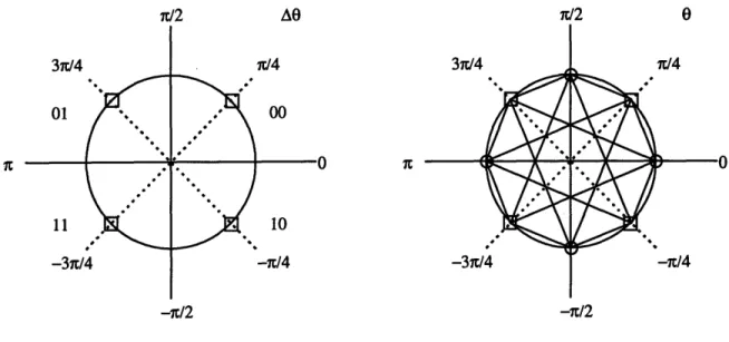
The PACS modulation method is 7c/4 shifted DQPSK (Differential Quaternary Phase Shift Keyed). Phase modulation is chosen since amplitude information is more vulnerable to fading environments, and allows hard limiting in the receiver, reducing complexity. Quaternary phase is chosen for its capacity increase over BPSK, 2 bits per symbol as opposed to 1 bit per symbol, and increased robustness over higher order PSK.

Finally, n/4 shifted DQPSK is chosen to guarantee phase changes every symbol, and prevent phase transitions through the origin of the complex phase plane.3 _Phase

transitions through the origin can occur in other systems when a phase change of +/- n; is

made. Figure 4-1 depicts the differential and absolute phase constellations of the modulation scheme. The differential constellation on the left shows the bit encoding of each symbol, and the absolute constellation on the right shows the resulting possible absolute phases, and possible transitions associated with each symbol. None of these design decisions are changed by asynchronous operation.

31d/4 01 11 -31x/4 Vt/4 00 31r/4 10 -7/4 1(/4

Figure 4-1 Differential (left) and absolute (right) phase constellations for x14 shift DQPSK

4.3 Error Check Coding

The error coding of the asynchronous transmitter is assumed to conform to the PACS standard. The PACS standard employs a cyclic redundancy check, essentially a parity check code. Work by Bellcore has determined that given the channel model

assumed, more sophisticated means of error correction offer little performance gain.4 The rules for choosing the optimal CRC code for PACS, using a 105 bit code word, 90 bit data and 15 bit CRC, are not affected by simply moving from isochronous to

asynchronous operation. However, if higher layer protocol work by others indicates that a different packet size is desirable for asynchronous operation, a new CRC code must be chosen.

4.4 Burst Size/Symbol Rate

As described earlier, PACS employs time division multiplexing to distinguish between multiple subscriber unit transmissions to a single RP. Thus, there is already a

concept of burst size in the PACS transceiver, since subscriber units transmit and receive according to a fixed, repeating time schedule called a frame. A PACS burst is 54 symbols in duration, or 106 bits, with successive bursts separated by 6 symbols of guard time. The 106 bits includes the 105 bit codeword and a pad bit. In order to preserve as many

elements of the existing receiver as possible, the 60 symbol PACS burst will be considered an atomic unit.

One parameter that must change to satisfy the FCC rules is the symbol rate. The standard PACS symbol rate is 192 kHz. Using a square root raised cosine transmit pulse shape with a roll off factor of 0.5, the transmission occupies a band at carrier +/- 1.5*96 kHz, a bandwidth of 288 kHz. The FCC rules require that any intentional transmitter use at least 500 kHz of bandwidth. The easiest way to map PACS into compliance is to double the symbol rate, occupying a bandwidth of 576 kHz. While it may be desirable to increase the symbol rate further, occupying more spectrum, it is more difficult to

implement such a design.

4.5

Coherent Demodulation

The existing PACS receiver uses coherent methods with good error performance in multipath fading environments. The PACS radio port has a free running oscillator that determines the carrier frequency. The PACS terminal receiver adjusts its oscillator to maintain phase lock with the radio port. The terminal receiver estimates the absolute phase of the transmission and performs carrier and phase recovery on the phase stream.

The current receiver uses digital block processing techniques to jointly estimate the symbol timing and carrier offset on a burst-by-burst basis. The symbol timing estimate is

made by accumulating a metric representing eye opening over a burst for all candidate sampling phases in the over-sampled receive stream. The carrier offset estimate is made by calculating the rotation of the differential phase constellation. The estimation window is 38 symbols long, a majority of the burst. Carrier frequency offset and phase offset estimates are further refined with a second order, critically damped loop. The differential phase information is extracted only after frequency and phase compensation of the absolute phase.5

The advantage of this coherent method is reduced sensitivity to local symbol impairments by averaging and accumulation over burst long periods. When fading occurs fast enough to change channel characteristics within a given burst, non-coherent methods become more attractive. However, for the channel model assumed, coherent receivers retain their advantage.

5. Problems of the Existing PACS Receiver

5.1

Transmission Overhead and Minimum Packet Size

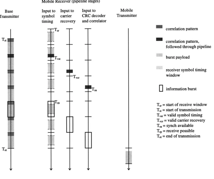
Since the existing PACS receiver employs block processing methods, several throw-away bursts are required before the receiver can synchronize with the transmission. The receive window must significantly overlap a valid transmission for the estimated parameters of symbol timing and frequency offset to be valid. During the first burst these parameters are estimated in the symbol timing process, during the second, carrier recovery converges on finer grain phase and frequency offsets and reconstructs symbols, and during the third, a CRC error check is performed. Figure 5-1 shows these 3 stages and the input

to a unique bit sequence, before the CRC check, provides a reference point for

synchronization. The CRC check cannot succeed unless the receiver has determined the start of the protected code-word in the transmission, so synchronization is necessary before any data can be successfully demodulated and decoded. Figure 5-2 assumes that the unique bit sequence is at the start of each transmission. Note that for one burst of data to be sent, 4 bursts of overhead must precede it. This is unacceptable in packet radio applications.

The reason for the receiver's long latency is its emphasis on low power

consumption and slow clocks. The speed of the parameter estimation operation is limited by the speed of the incoming transmission, but subsequent carrier recovery and decoding are performed at the symbol and bit rates. By performing these operations at a faster rate, latency can be reduced.

A Joint symbol timing and Carrier recovery by C Synchronization Slip / D

frequency offset : second order loops Error Detect by staggered

estimation CRC decoders

A: Over sampled IF stream (20 samples per symbol)

B: Absolute Phase stream at symbol rate

C: Symbol stream at symbol rate (2 bits per symbol) D: Error checked bit stream at bit rate (2x symbol rate)

Base Transmitter

Mobile Transmitter Mobile Receiver (pipeline stages)

Input to Input to Input to symbol carrier CRC decoder timing recovery and correlator

Tsr Tyst _{_}

-

-Figure 5-2 Overhead requirements of current design.

5.2

Demodulation /Decode Latency and Terminal Response Time

The receiver latency poses another problem when viewed in the context of the Asynchronous spectrum etiquette. The inter-burst gap requirement specifies that the gap between successive transmissions of cooperating devices is less than 25 us. Given that a transmission occurs as depicted in Figure 5-2, the spectrum must remain occupied until the

terminal is able to respond. Due to approximately three bursts of latency, data is not correlation pattern correlation pattern, followed through pipeline burst payload

receiver symbol timing window

U

Tsr = start of receive window Tt = start of transmission Tst = valid symbol timing Tvr = valid carrier recovery Tsa = synch available Tp = receive possible Tet = end of transmission

Tst

available to the terminal until two bursts after the transmission has ceased. As a result the base must transmit 2 wasted bursts after the information burst. Note that 7 bursts had to be transmitted to send one burst of information.

Note that there are two related problems, excessive processing latency and excessive overhead. However, even if latency is drastically reduced, the limiting case on overhead is still one burst. One burst of overhead is required to ensure that a valid transmission overlaps the symbol timing estimation window. So some novel approach is required at the symbol timing stage.

6. New Receiver Techniques

6.1

Media Access Control Perspective

The challenging environment of an asynchronous data network requires a receiver with low latency and low synchronization overhead. For this reason, the network design decisions made in media access control (MAC), determine the requirements imposed on the receiver. The FCC rules for cooperating devices constrain MAC layer design, and in turn, receiver design. Two MAC layer methods for meeting the inter-burst gap rule impose very different requirements on receiver latency. Furthermore, different scenarios for RP / terminal cooperation lead to different overhead requirements.

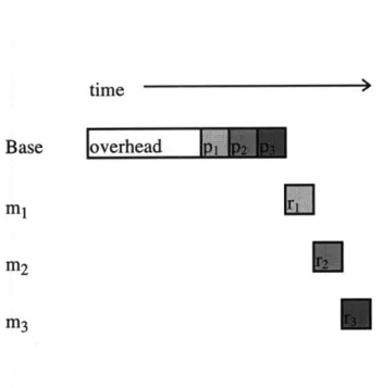
Two approaches to meeting the 25 us inter-burst gap rule impose weak and strong constraints on latency. The first approach is to allow any two terminals to act as a

than 25 us. This requires a given terminal receiver to be able to demodulate and decode a transmission within 1 burst and 25 us, with enough time remaining for the terminal to recognize an identifying user address and possibly initiate a transmission, all before the 25 us has expired. A second approach is to employ a polling scheme where the base sends a series of packets, each of which requires a response from a different mobile terminal.6

Given a system of a base and 3 terminals, let 3 packets be pi, P2, and p3, and three mobile

terminals be mi, m2, m3, as depicted in Figure 6-1. The base first transmits some required

overhead followed by packets pi through P3. Assuming a receiver latency of

approximately 3 bursts, packet px will be decoded by mobile mi while the base is

transmitting packet p3. The mobile can then send response rl. During response ri, mobile m2 decodes packet p2 and is ready to respond with r2 within the following 25 us. In this

manner an arbitrary number of packets can be "piggybacked" to work around any hardware latency. However, it is desirable to minimize the number of piggybacked transmissions, since the failure of any given mobile terminal to respond breaks the chain and violates the 25 us constraint, allowing other groups to seize the spectrum. From this example one can conclude that the length of the polling chain is the smallest integer

number of bursts greater than the receiver latency, or Flatencybrsts) So even if a

polling scheme is employed, it is desirable to minimize the length of the polling chain, and consequently, the receiver latency. Note that this imposes a weaker constraint on latency than the non-polling approach, since any latency between n and n + 1 bursts in duration, where n is an integer, still leads to a polling chain of n + 1 terminals.

time

Base loverhead

Figure 6-1 Polling Access piggybacking transmissions

Different scenarios for device cooperation also impact the overall overhead to payload ratio. While the spectrum usage is, in general, asynchronous, a cooperating group can use it in a synchronous, slotted manner during its possession. For example, one could require the base to be the first transmitter in the cooperating group. The base would gain spectrum access asynchronously, but all cooperating mobile terminals could then

synchronize to the base's transmission, and communicate synchronously in burst-size slots for up to 10 ms. While there may be carrier and clock offsets between different terminals, they are unlikely to drift out of synchronization within 10 ms (64 bursts), and there are digital phase locked loop methods from PACS telephony that would keep them

synchronized. As a result, the transmission overhead required for synchronization only occurs at the start of the group's exchange. The longer the exchange lasts, that is the closer to 10 ms duration, the lower the overhead ratio. As a result, it may not be worthwhile to decrease synchronization overhead only slightly, at the cost of increasing complexity significantly.

ml

m2

6.2

Reducing Latency

Upon consideration of the existing pipelined receiver it has been determined that some modules can operate at much higher clock rates, and some of the pipelined modules can begin processing before previous stages are done. Together these two techniques can yield significant latency reduction.

The effect of these techniques can be depicted using a two dimensional graph. On the vertical axis is time, measured in channel symbols, increasing downward. On the horizontal axis is the symbol number in a given burst that is being processed, increasing to the right. Therefore, solid lines depict the progress of each stage in processing the burst. The closer the slope of a given line to being horizontal, the higher the processing speed of that stage.

First, consider the performance of the existing design. Table 6-1 describes

significant times in the processing of the received stream. It also characterizes the type of inputs entering each stage, as operations transform the data stream.

Description

Start of oversampled IF data entering receiver, where high pass filtering, digital mixing and bandpass to phase conversion occurs.

Start of oversampled phase stream entering symbol timing estimation, where eye opening metric for each sampling position is accumulated over window.

Symbol timing estimates of best sampling position and frequency offset corresponding to sampling position with greatest eye opening metric are available.

Phase stream downsampled to symbol rate at estimated symbol timing position.

Time

TA1

TA2

TA3

TAs

Ts1

Table 6-1 Reference time labels in demodulation and decoding.

Figure 6-2 illustrates the latencies of each stage, using the reference time labels. Note that the symbol timing estimate used to downsample the oversampled phase stream is available at time TA3, well before it is used at time TA4. As a result, carrier recovery could start earlier. Also, note that all the data to be processed by the carrier recovery and CRC decoding stages (TB1 to Tc2) is available at time TA5. Therefore, while the symbol timing

stage is constrained by the channel symbol rate, the carrier recovery and decoding stages can be run at an arbitrarily high multiple of the symbol rate, r. This is represented

graphically by flattening the slope of the carrier recovery and decoding lines. The case where r is 2 is depicted on the right of Figure 6-2. The benefit of increasing r is

constrained by the fact that the carrier recovery and decoding stages cannot process data before its available. This violation could be represented by allowing the carrier recovery line to cross the symbol timing line. Thus, time TA5 imposes a limit on the minimum latency.

End of oversampled phase stream entering symbol timing estimation.

Start of chosen phases at symbol rate entering carrier recovery, forward compensation loop initialized with frequency offset estimate.

Finer grain frequency and phase offset estimates convergent, backward compensation loop initialized, forward loop continues

Carrier recovery complete, 2 bit symbols serialized into bit stream at bit rate

Bit stream delayed by 6 bits (3 symbols) enters CRC decoder, delay is nominal, allows compensation for slips of the actual position of codeword -6 bits, -4 bits, -2 bits, 0 bits, +2 bits, +4 bits, +6 bits

on symbol on symbol latency 0 11 30 49 60, latency 0 11 30 49 60., (symbols) " I I (symbols) u

Figure 6-2 Existing design (left), and variable processing improvement (right).

1 50 51 81 82 operation operation 61 62 92 122 125 165 A •J., , TA4

9

The following derivation, developed with Research Scientist, Gregory Pollini, quantifies the minimum bound on the latency of the current receiver, expressed in terms of the channel symbol rate and r.

Let the reference time TAl equal 0. Let the duration of one burst, or 60 symbols, equal T. The filtering and mixing operations that follow are implemented with a 5 tap FIR filter, and a set of look up tables for trigonometric functions, all at the oversampled rate. The latency of the filtering, mixing and conversion to phase operations is therefore less than one symbol. To obey symbol boundaries, it is most convenient to round the delay to

1 channel symbol, so that TA2 = T. The symbol timing metric accumulation window

60

50

is 38 symbols long, starting 11 symbols into the burst, so TA3 = - T. Since the burst is 60

61 60 symbols long, TA is 60 symbols after TA2, so TA5 = - T.

60

The main distinction between the existing design and the improved design is that the carrier recovery process can start as early as a symbol delay after time TA3, when the

estimates used to initialize it are ready. This symbol delay is incurred in the phase stream

50

downsampling process. Thus, in the improved design, TA4 = TA3 = - T, and TB1 =

60

51 T. Assuming the most general case, in which r _{is an arbitrarily high multiplier, the} 60

carrier recovery process could overtake symbol timing. The processing rate of carrier recovery would then have to slow down to the rate of symbol timing to avoid overtaking

it. So TB3 = max[TB1 +

1 62 ₆₂

ST,-TI ._{The limit imposed by TA5 is now apparent, as - T}

r 60 1 60

is the one symbol downsampling delay after TA5.

Decoding can begin 3 symbols after the backward compensation loop is finished. Since the backward loop is processing stored phases from the first half of the burst, it is

1 3

not limited by TA5, allowing decoding to begin at Tc, = TB+ T+ 1 3 T. There is a

r 60r

possibility that decoding could also overtake symbol timing, so Tc2is limited by TA5 such

that Tc2 = max51 +

1,62

r r

Figure 6-3 summarizes these results and expresses

time in terms of channel symbols.

TA2 =1 TA3 = TA4 = 50 TBI =51 TA5 =61 TB3= max[51 + ,62 63 Tc, =51+ -r Tc2 =max 51+ 12362+ 3

The final expression for the minimum latency of the current receiver using variable

processing rates is TC2 = max[5 1+13 ,62+

]

Latency vs r

120

Figure 6-4 Latency as a function of variable processing rate

6.2.2 Required Buffering

As pipelined designs, both the original receiver and variable rate receiver require memory elements between successive stages. These elements are implemented in a straightforward manner in the original design, since they are read from and written to at

23 I· | I I | I I I

-- ---- -

-the same rate. However, in a variable rate design, more complexity is introduced, as separate addresses must be maintained for fast reads and slow writes. Also, in the overtaking case, the reads themselves may slow from one rate to another.

For example, in the original design, most of the memory elements are implemented in a first in first out (FIFO) or last in first out (LIFO) manner. A FIFO RAM stores oversampled IF data during the one burst latency of symbol timing. A LIFO RAM stores downsampled phases during the half burst latency of carrier recovery convergence. A reorder RAM stores compensated symbols as they available during the second half of carrier recovery, making them available in the correct order during the next burst. Finally, another FIFO RAM stores the serialized bit stream during the one burst latency of CRC decoding.

Many of the memory elements in a variable rate design can be implemented in a similar manner, as long as r is small enough such that carrier recovery does not overtake symbol timing. In this case, only the storage between symbol timing and carrier recovery requires independent read and write addresses. Furthermore, while the reads from and the writes to that memory occur at different rates, they occur at constant rates. All

subsequent memories operate uniformly at the faster rate. However, if r is large enough to allow carrier recovery, or even decoding to overtake symbol timing, the fast memory reads must slow down to the symbol rate. This implies that all of the memories would have to support two read rates.

In order to quantify the latency / complexity tradeoff, examine Figure 6-4. Note that there is a diminishing return as processing speed increases. In a polling strategy such

as that suggested by MAC layer considerations, the most significant changes in latency occur for values of r where the amount of latency crosses a burst boundary. Since the latency remains between 1 and 2 bursts for any r greater than 2, there is little gain in performance for the large gains in complexity associated with very fast processing. The highest r for which carrier recovery does not overtake symbol timing, is that which

60

satisfies the equality, 51+ -= 62, obtained from the end time of carrier recovery, TB3, r

60

meeting the symbol timing constraint, TAS. Therefore r = 6 = 5.45. For implementation

11

purposes integer multiples of the symbol rate or desired, so for r = 5, the latency is 75.6 symbols, or 1 burst and 40.625 us. If MAC layer work determines that a non-polling strategy is desired, such that successive transmissions are not piggybacked, a latency close to one burst is required to meet the 25 us inter-burst gap constraint. If so, then the highest

r for which carrier recovery overtakes symbol timing but decoding does not, is the

123 3

discontinuity in the total latency expression at 51+ = 62 +-. This yields

r r

120

r =

-j

11

burst and 5.99 us. Choosing r > 10 leads to excessive complexity in implementation of the decoder, with little reduction in latency.

6.3

Reducing Synchronization

Overhead

Given the latency reductions already stated, the overhead requirements must be reevaluated. Given a receiver with very low latency, on the order of one burst,

piggybacking may not be required. As shown in Figure 6-5, now only 3 bursts need be transmitted for 1 burst of information to be sent.

Mobile Receiver (pipeline stages)

Input to Input to Input to

symbol carrier CRC decoder

timing recovery and correlator T, -- Tsr Mobile Transmitter a correlation pattern correlation pattern,

followed through pipeline

burst payload

receiver symbol timing window

U

T, = start of receive window Tt = start of transmission

st = valid symbol timing TVr = valid carrier recovery

Ta = synch available Trp = receive possible

Tet = end of transmission

Figure 6-5 Overhead requirements of reduced latency receiver

6.3.1 Correlation Position in Burst

A simple method for reducing the overhead involved in synchronization, is to accept at least one burst of overhead and fill it with a series of synchronization words. As a result, the sliding window correlator will match on the earliest valid pattern, allowing the earliest possible synchronization. Each pattern would have to be distinct so that the correlator would be able to resynchronize accordingly. The benefit of this modification alone is unclear, since the correlation may occur after the second transmitted burst has already begun. In that case, synchronization would still occur at the start of the third Base

Transmitter

Tst,

transmitted burst. The benefit of this method used together with others is studied further in simulation.

6.3.2 Parallelism - Multiple Staggered Receive Windows

Another method to reduce synchronization overhead, is to use a set of parallel demodulators with staggered symbol timing estimation windows. At one extreme is a set of ten demodulators and decoders, with windows staggered by 6 symbols each. Together this set could cover all positions of burst alignment that are within the slip correction range of each decoder. This configuration could entirely eliminate the need for one overhead burst. Further study is required to specify the minimum amount of parallelism required, but the case of 3 demodulators is instructive. This configuration, together with an initial burst filled with synch words, could reduce synchronization overhead to one burst.

6.3.3 Half Burst Demodulator

Finally, by shrinking the block size over which demodulation occurs, it becomes more likely that the first burst of a transmission will overlap a large fraction of the smaller symbol timing estimation window. For example, if the demodulator operated only on half bursts, with a smaller symbol timing window and half burst carrier recovery, the receiver would be more likely to resynchronize by the start of the second transmitted burst. The obvious consequence of this approach is worsened error performance, but simulation to determine the extent of performance loss is required. Also, analysis of the metrics used in symbol timing, and analysis of the carrier recovery loops, provides insight into the

7. Analysis of Channel Estimates and Carrier

Recovery

The existing demodulator treats each burst-sized block independently. This has the advantage of yielding averaged channel measurements well correlated to the channel at the measurement time, which is important in the case of a slowly time varying channel. Also, the short, burst-long measurement time allows a low latency implementation. However, for a non-varying channel, averaged measurements over a longer time period are more accurate, ostensibly permitting lower error rates. The price paid is susceptibility to time varying channels, where a single averaged measurement does not closely represent the channel at different times. Also, the longer measurement time requires a higher latency implementation. Thus, performance and latency tradeoffs are apparent in choosing the duration of the measurement time.

In addition, in examining receiver performance in asynchronous applications, the case where the measurement window does not fully overlap the time period of a valid transmission is of particular interest. In this case, the averaging measurements are degraded by the initial ambient noise of the channel, and are further degraded by the shortened period of available valid transmission. Furthermore, in the carrier recovery stage, the initial noise delays loop convergence on phase and frequency offset estimates, and shortens the length of valid input to drive the loop to convergence. As a result, insight into the sensitivity of channel measurements and carrier recovery to noise is required. This insight can clarify the performance tradeoff involved in the half burst demodulator suggested.

Finally, another consequence of a block oriented demodulator, is that symbol errors are necessarily incurred at block boundaries. Between blocks, information such as differential symbol encoding is lost as memory elements are cleared. Thus, while shorter window demodulators may be discussed for the purpose of synchronization, they are not appropriate afterwards, when burst-long CRC codewords must be preserved intact for successful decoding.

7.1 Symbol Timing Quality

Index

(QI) and Frequency Offset

Estimation

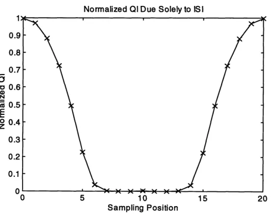
As mentioned earlier, the PACS system uses square root raised cosine pulse shaping in transmitting the modulated stream. This pulse shape does have some inter-symbol interference (ISI), even when sampling at pulse maxima. However, a narrowband receive filter is employed, with a frequency domain characteristic resembling the square root raised cosine response. The cascade of these two characteristics ideally yields a raised cosine characteristic, leading to a no-ISI "Nyquist" pulse shape at the receiver. In the time domain, each raised cosine pulse is ideally infinite in time, however, each zero crossing of a given pulse coincides with the peaks of neighboring pulses. Thus, if the receiver chooses the correct sampling instant over a symbol period, there is no ISI. Figure 7-1 depicts a series of raised cosine pulses. Note that the pulse amplitude decays rapidly in the time domain. Thus, the pulse centered at t = 0, which is overlaid with contributions from the 2 pulses before and after, encounters interference typical for any given symbol.

Zero-ISI Raised Cosine Pulses (D a . E -2 -1 0 1 2 Time (symbols)

Figure 7-1 Zero ISI Pulse Shapes

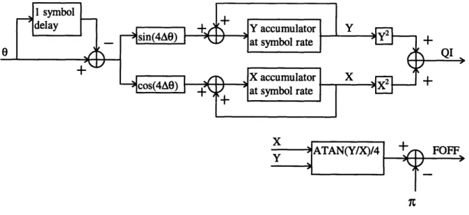
It is the goal of symbol timing to estimate the correct sampling offset, updating the estimate each burst. This is done in the digital domain, in the following manner for each burst. An analog IF input is over-sampled with 4 bits of precision at a rate 20 times the symbol rate. Through a series of signal processing methods a quantized instantaneous absolute phase stream at 10 times the symbol rate is extracted from the over-sampled IF stream. Phases are represented with 8 bits of precision, proving 256 levels between -7c and x. At 10 offset positions this phase stream is differenced yielding 10 symbol rate

differential phase streams. A QI metric is obtained for each sampling offset by operating on the corresponding differential phase stream, and the sampling offset with the highest QI is chosen for symbol timing. Figure 7-2 illustrates the band pass to phase stream

phase stream while a new decimation offset is chosen on the basis of QI. A frequency offset estimate and a symbol rate absolute phase stream are inputs to the next stage, carrier recovery. While this figure accurately represents the functionality of the implementation, the implementation is more hardware efficient.

Im I

IF20x IFAC Digital mixing into I Image reject filtering ATAN(Q/I) phase20x

DC Filteringand Q components Q

Figure 7-2 Bandpass to Phase Conversion

The QI metric is best understood as the magnitude squared of a vector sum of a series of unity magnitude vectors. Given an absolute phase stream, a differential phase stream is easily computed. In the absence of a frequency offset, when sampling at the correct sampling instant, the only acceptable values of differential phase should be clustered near the constellation points of +/- 7t/4 and +/- 37c/4. Multiplying any of these

multiplied by 4, 4A0, can be considered a stream of unity magnitude vectors. Noise,

modeled as additive phase noise, may perturb each vector slightly from 7T. A vector is

constructed by summing a series of the 4A0 vectors. Assuming zero mean noise, applying

the law of large numbers, the noise should sum destructively while signal component sums constructively, yielding a large vector in the direction of 7r. The duration of the

measurement time directly impacts the validity of the above assumptions, since over short periods of time a given noise sequence may not sum to near zero. Also, the amount of valid transmission within the measurement window affects the constructive summing of signal components. The less valid transmission that is accumulated, the closer the maximum QI will be to the smaller erroneous QIs. The less invalid transmission that is accumulated, the closer the erroneous QIs will be to the maximum QI. Figure 7-3 illustrates the computation of QI for a given symbol rate phase stream.7

x

X ATAN(Y/X)/4 + FOFF

Sampling at a position offset from the correct one, ISI is encountered. It is no longer true that differential phases will be near constellation points. The effect of ISI can also be modeled as a data dependent noise, which increases as the offset from the correct sampling point increases, until one passes the center of the symbol and nears another sampling instant. Instead of performing this analysis, an empirical QI as a function of sampling offset, without noise, shows how ISI leads to a destructive vector sum away from the correct sampling point. Figure 7-4 was generated in simulation neglecting quantization, using an appropriately modulated, noise free, random bit sequence, with QI accumulated over approximately 960 symbols and normalized to a maximum value of 1. Assuming noise still sums destructively, a maximum QI can be used to choose the correct sampling instant.

Normalized QI Due Solely to IS I

1 0.9 0.8 0.7 a o 0.6 N . 0.5 o 0.4 Z 0.3 0.2 0.1 0 0 5 10 15 20 Sampling Position

In the presence of frequency offsets, the differential phase constellation is rotated

by some angle 8. This is because a frequency offset can be represented as a constant

derivative of phase, so in some time interval At there is a fixed phase change AO. A given

frequency offset then leads to a fixed phase change 6 over each symbol interval, simply

rotating the differential phase constellation by 8 radians. Therefore, the magnitude

properties of the QI vector sum without frequency offset, also apply in the presence of a frequency offset. However, with a frequency offset, the angle of the vector sum for the

correct sampling instant will no longer be 7r radians. Instead, at the correct sampling

instant, each vector of the 4A0 stream generally points toward 7; + 48, and so will the vector sum. So while QI, the magnitude of the vector sum, indicates the correct sampling instant, the deviation of the angle of the vector sum from nt indicates the frequency offset.

The limitation of this method of frequency offset estimation is also apparent, since if 48

exceeds nc, a positive frequency offset would alias into a negative one and vice versa. This

translates into a maximum frequency offset of +/- i/4 radians per symbol, which at a symbol rate of 384 kHz yields a frequency offset of +/- 48 kHz.

In order to investigate the effect of noise on the QI metric, several assumptions may be made. First quantization error will be neglected for initial ease of analysis.

Second, the transmitted data sequence will be considered independent of the noise. As a result, the effect of ISI at sampling positions offset from the correct one will be treated as independent of the noise, since ISI is a deterministic function of the transmitted data. Furthermore, the effect of ISI may be considered a deterministic function of sampling offset conforming to the simulation results cited previously. While this is only directly

valid for very long accumulation periods with random data, it can be made valid by construction of appropriate short data sequences. Since user data will be preceded by some form of synchronization sequence, this sequence can be designed to yield ISI conforming to the assumption. Third, frequency offset will be considered a fixed differential phase offset within the estimation range, so that the case without frequency offset can be considered without loss of generality. Given these assumptions, one can derive some expressions for QI at the correct sampling point to see its functional dependence on noise terms.

Oi = s + n, + f,

f,=O

QI=

i4AO

e

2

=

cos(

+ 4AnJ +

·

(

= ( cos(4An) + Isin(4An)

This expression for QI demonstrates the effect of several types of phase noise. If 4An is uniformly distributed, then QI is very unhelpful, as it approaches zero. If it is gaussian distributed with zero mean, QI will approach N2 in the absence of noise, where N is the number of symbols summed. The uniform distribution is a very pessimistic case, however. This may be justified with some empirically obtained cummulative density functions, that

reveal that white gaussian phase noise is a good approximation for a wide range of signal to noise ratios. First, one may generate a large number of independent trials of complex noise phasors with rayleigh distributed amplitude and uniform phase. For the empirical method, 100,000 trials were performed. Then, a signal component can be considered with unity magnitude and zero phase, or real part one and imaginary part zero. A resultant random variable can be computed for each trial that is the sum of the noise and signal components. The phase of this resultant for each trial is the phase domain noise of concern. An empirical CDF can be constructed based on the empirical distribution of the many trials, and this CDF can be compared to the empirical CDF for a gaussian with matching variance. If signal-to-noise ratio (SNR) is defined as 10logio(var(S)/var(N)),

and this is used to choose the rayleigh parameter a, the gaussian approximation can be tested at various SNRs. Figure 7-5 depicts the empirical CDFs obtained at two SNRs, and the difference between the rayleigh and gaussian ones. It becomes apparent that the approximation is least accurate in the tails of the distribution, or at the outlying values. However, the QI metric seems valid for the type of noise expected, at reasonable values of SNR.

CDFs SNR = 12 dB 1 0.8 0.6 0.4 0.2 I. 0 Phase Error SNR = 12 dB 0.5 P 1 0.8 0.6 a. 0.4 0.2 0 0 0 Phase Error SNR = 6 dB 0.5 P

7.2 Carrier Recovery Second Order Loop

The purpose of the carrier recovery stage is to refine the frequency offset estimate and converge on a phase offset estimate. The stage then compensates the symbol rate absolute phase stream for these offsets, extracting the symbol information as a sequence of di-bits. This is accomplished using a second order loop, with one state tracking phase offset, and a second state tracking frequency or change in phase offset. The frequency

V -5 -2 I 0.5 0 -0.5

Figure 7-5 Empirical CDFs at several SNRs

c

CDFs SNR = 6 dB

]

t

offset state is initialized with the frequency offset estimate obtained in the symbol timing process, while the phase offset state is initialized to zero.

In the absence of frequency offsets, the correctly sampled, symbol rate absolute phase stream should ideally take values near the eight absolute phase constellation points. This would suggest that there are eight decision regions, however, there are actually only four. If one considers the absolute phase constellation at odd intervals of time and at even intervals of time separately, one obtains two constellations of four points offset by 7t/4 radians. This is depicted in Figure 4-1, with one sub-constellation denoted with boxes, and the other with circles. As a result, before the absolute phase stream is fed to carrier recovery, it is derotated. In other words, given the starting symbol phase in a sequence, n/4 radians is added to every other symbol phase, rotating one of the 4 point constellations

to overlap the other. This derotated absolute phase stream, Od, has a simple 4 point constellation. The presence of frequency offsets simply causes the constellation to rotate from one symbol to the next.

The second order loop tracks phase and frequency offsets by driving phase error to zero. Phase error is defined as the phase difference between a given derotated symbol phase and the nearest constellation point. The loop is depicted in Figure 7-6. Again, the figure conveys the loop's functionality, but there are implementation specific details that are not shown. For example, the difference between Od(k) and the phase state register p(k) yielding error e(k), is only taken modulo one quadrant of phase, to consider error only from the nearest constellation point. As the figure shows, phase error is fed back with appropriately chosen gains a and b, to update phase and frequency offset estimates.

Loop analysis reveals that with the proper choice of a and b, e(k) will converge to zero. In the implementation it is assumed that the loop will converge within 30 symbols of iteration, with the input stream buffered during this convergence time. In the full burst receiver implementation, the loop continues forward through the remaining 30 symbols of the burst, while a functionally identical loop is run back through the buffered 30 symbols. The backward loop is initialized with the convergent state of the forward loop, reversing the sign on the frequency state for time reversed operation. This is the compensation stage, where the difference between 0d(k) and the phase state p(k), is now considered over the full range of phase, not simply for error information. The resulting forward and

backward phase streams should have a 4 point constellation on the axes of the complex plane. The constellation is rotated by n/4 radians by adding tr/4 to each phase, and then the upper 2 bits of the resulting phases determine which of 4 symbol decision regions each phase is in. After some latency required for reordering this dibit stream to match its order of arrival, the reordered dibit stream is rerotated and differentially decoded to extract the symbol information.

Figure 7-6 Carrier Recovery Second Order Loop

A key issue is the effect of noise on loop convergence. Also of issue is the case where the 30 symbol convergence window does not fully overlap a transmission. The presence of initial noise delaying convergence, coupled with a shorter information

sequence for achieving convergence, raises the possibility that the loop will not converge. To study these issues, one may model the loop with a z-domain transfer function. Solving the difference equations obtained for the above loop, and expressing results in the D

domain (D = z-):

E(D) (1- D)2

By inspection the zeros are both located in a double zero at zz = 1. Solving for the poles, one obtains:

2-a+_

±a-abi

DP 2-.(1+b-a)

In order to obtain a transfer function with desirable step response characteristics, such as short settling time and low overshoot or oscillation, a and b can be chosen such that the loop is critically damped. This constrains both poles to be a double real valued pole at zP

= (2-a)/2, with b equal to a2/4. For a stable response, the poles must be within the unit circle, so a > 0. This is consistent with a negative feedback configuration. Furthermore, for greater immunity to noise and oscillation, a < 1. For ease of implementation, a and b are chosen as fractional powers of 2, 2-k, since these multiplications can be represented with simple binary right shifts. Finally, the larger a and b are, the closer the poles are to the origin of the z-plane, and the faster the loop will converge. Based on these tradeoffs, a =

1/2 and b = 1/16, placing the double pole at z = ¾. Figure 7-7 shows the pole and zero locations chosen for the carrier recovery loop.

e{z}

In the absence of noise, this loop can track step inputs or ramp inputs, with error converging to zero within 30 iterations. Step inputs correspond to a derotated phase stream with a constant phase offset, while ramp inputs correspond to a derotated phase stream with a constant frequency offset. Figure 7-8 demonstrates error convergence for step and ramp inputs with slightly perturbed initial conditions, for both the chosen fast poles and alternate slower poles.

Step Input

Step Response

1.5

1

oUU

Ramp

Input

Sample

Figure 7-8 Step and Ramp responses for carrier recovery loop

20 40 6

Ramp Response

/

i00Pl

\

Sample

The final value behavior of the loop can also be understood from a frequency domain perspective. The loop transfer function has a notch characteristic in magnitude. Both the step and ramp inputs have most of their spectral energy near dc, as a result, the cascade of these systems with the loop leads to a zero output.

The effect of noise on loop convergence must be considered in two steps. First, when the receive window does not fully overlap the transmission, the initial input to the loop is noise. Since the loop has state including only the last two inputs at any given time, the initial noise can be considered solely as perturbing the loop's initial conditions, before the start of valid data. Given valid symbol timing, the loop's frequency state is initialized to a value close to its final one, and the phase state is arbitrarily initialized to zero. The effect of initial noise is to perturb these states. Second, additive noise on the valid

derotated phase stream may affect loop settling time and oscillation. By linearity the loop output can be considered a sum of responses to individual loop inputs. The above analysis shows that the output due to signal component converges to zero, so the output due to the noise component can be considered independently. Given low feedback gains, a and b, after convergence the loop error closely matches the additive noise. Again a frequency domain perspective adds insight. A wide-band noise process has energy beyond low frequencies that passes unchanged through the loop filter, and only components near dc are removed from the noise. The lower the feedback gains, the closer the poles become to the unit circle, and the loop filter becomes a more selective notch, removing components only very near dc. Important questions then, are what input noise is expected, and what is the critical noise energy that leads to unacceptable error oscillation. Unacceptable

oscillation has amplitude approaching xi/4 radians, or an envelope of 7r/2 radians, since error spikes of this magnitude lead to aliasing of one symbol for another.

This analysis of carrier recovery provides insight into a "critical" offset, the time offset between the demodulation window and the transmission after which demodulation is no longer reliable. As the response plots show, at least 20 symbols of valid input are required for the loop to converge, corresponding to a critical offset of 10 symbols. While the demodulator may succeed under offsets greater than 10 symbols, it is not likely to succeed under offsets greater than 15 symbols. In this regime, even if symbol timing is successful, carrier recovery is likely to be highly divergent.

8.

Whole Burst Receiver With Backward Buffering

One approach in modifying the receiver is to accept the synchronization overhead, but buffer the lost transmission, so that after synchronization, the receiver can simply run through the buffered data. Using this approach, the transmission that is used during synchronization is not wasted, and its information can be recovered after the fact. The disadvantage of this approach is the large amount of buffering required. Another disadvantage is that the terminal may waste time at the end of a transmission processing what remains in its buffer. This is the case unless the terminal can begin responding as soon as the base completes its transmission, while the terminal is still processing buffered data. Finally, this approach imposes a limitation on the minimum transmission size. The transmission must be at least as long as the long synchronization time, otherwise the terminal will be unable to synchronize, and any buffering is wasted. Actually one may

require a slightly longer transmission to allow the terminal time margin for initiating a response.

The large amount of buffering required renders this approach undesirable. Since the start of the transmission is not known initially, the buffer must store data at the over

sampled rate, since the block demodulator would induce errors at window boundaries. Storing approximately 4 bursts or 2400 samples of 8 bit phase data would require an additional 18.75k of memory. Therefore, this approach alone is inefficient. However, if combined with the reduced latency implementation, only 2 bursts or 1200 8-bit samples, totaling 9.375k need be stored. In general, this approach becomes more desirable if combined with a reduced synchronization time receiver, reducing the amount of buffering required.

9. Half Burst Receiver

A more hardware efficient approach for reducing synchronization time is to employ a shorter-window receiver. The primary benefit to this approach is that a shorter measurement period allows a higher measurement frequency. If the start of the

transmission is greatly offset from the start of a given measurement window, the first partially overlapping measurement will be unreliable. However, since the window is short, the next fully overlapping measurement occurs and ends soon enough after to allow rapid synchronization. As discussed earlier, the disadvantage of this approach is less reliable symbol timing and frequency offset estimates, and estimates and carrier recovery more sensitive to noise. The tradeoff then is faster synchronization time for higher probability

of missing a transmission. Two important questions then, are how fast can

synchronization be, and how much does the miss probability increase.

A convenient choice for short window length is half of a burst, since that would

permit an implementation of both a half and a whole burst receiver with a common data path, but with different control paths. This common architecture is important because

after synchronization, a whole burst receiver is more desirable. The half burst receiver would introduce errors between half burst blocks at the window borders. Also, the whole burst receiver would mostly likely have better symbol timing and frequency offset

estimates from the longer measurement time, given that the channel is flat over a given burst.

Even with a half burst receiver in the pre-synchronization stage, multiple synchronization words must be transmitted to permit rapid synchronization. If the first partially overlapping measurement window fails to provide valid symbol timing, even if the next window yields valid symbol timing, there must be another symbol sequence available to synchronize to. While there are highly refined methods for choosing the optimal length and values of synchronization sequences, the PACS frame synchronization sequence may be considered as a starting point. The PACS frame-sync sequence is 24 bits, or 12 symbols long. One could adapt this sequence to choose a set of several synchronization sequences, starting the transmission with a series of synchronization words. The receiver may then employ a different sliding window correlator for each expected sequence, determining the offset of its measurement window based on which correlator obtains a match. Following a correlation match, the receiver can realign its window and begin full