Crack Propagation in Tool Steel X38CrMoV5 (AISI H11) in SET Specimens

HAL Id: hal-01666707

https://hal.archives-ouvertes.fr/hal-01666707

Submitted on 25 Sep 2018

HAL is a multi-disciplinary open access

archive for the deposit and dissemination of

sci-entific research documents, whether they are

pub-lished or not. The documents may come from

teaching and research institutions in France or

abroad, or from public or private research centers.

L’archive ouverte pluridisciplinaire HAL, est

destinée au dépôt et à la diffusion de documents

scientifiques de niveau recherche, publiés ou non,

émanant des établissements d’enseignement et de

recherche français ou étrangers, des laboratoires

publics ou privés.

Crack Propagation in Tool Steel X38CrMoV5 (AISI

H11) in SET Specimens

Masood Shah, Catherine Mabru, Christine Boher, Sabine Le Roux, Farhad

Rezai-Aria

To cite this version:

Masood Shah, Catherine Mabru, Christine Boher, Sabine Le Roux, Farhad Rezai-Aria. Crack

Prop-agation in Tool Steel X38CrMoV5 (AISI H11) in SET Specimens. Advanced Engineering Materials,

Wiley-VCH Verlag, 2009, Fatigue and Plasticity, 11 (9), pp.746-749. �10.1002/adem.200900044�.

�hal-01666707�

Crack Propagation in Tool Steel X38CrMoV5 (AISI H11) in

SET Specimens**

By Masood Shah,* Catherine Mabru, Christine Boher, Sabine Leroux and Farhad Rezai-Aria

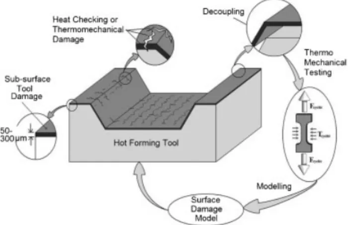
An approach is proposed for the study of sub-surface damage experienced in hot-forming tools during machining. For example, studies of pressure die-casting dies[1,2]have shown that the surface damage in tool steels extends from the surface down to 50–300 mm into the bulk material (this thickness will hereafter be referred to as the ‘‘surface’’). It is also known that the properties of materials of low thickness may be different from those of bulk materials.[3–5]It is, therefore, proposed that the crack initiation and propagation behavior of the surface be studied separately from the bulk (Fig. 1). Initial results obtained from the testing procedure are presented.

Material and Specimen Preparation Material

The experiments are carried out on a hot-work martensitic tool steel, X38CrMoV5 (AISI H11), which was delivered free of charge by Aubert and Duval in the form of forged bars of 60 mm square section. It is a low Si and low NMP content, 5% chrome steel principally used in the high-pressure die-casting (HPDC) industry. The steel is quenched and double tempered to a hardness of 47 HRC and syof 1 000 MPa. The chemical

composition is given in Table 1.

Specimen Preparation and Test

All SET specimens are machined by wire-cut electro-erosion on a Agiecut 100D wire-cut machine (Fig. 2a). The flat surfaces of the specimens are then ground parallel on an LIP 515 surface grinder. Finally, specimens are polished on a metallographic polisher Buehler1Pheonix 4000 to obtain a mirror finish with a 1 micrometer grit diamond paste. A grid of 0.10! 0.10 mm is marked on the polished surfaces (Fig. 2b).

The crack propagation experiments were carried out on a servo-hydraulic universal testing machine Walterþ BAI LFV 40 at an ambient temperature of 258C. Propagation is optically observed in situ with a Questar1 observation microscope (0.0012 mm resolution) without interruptions. Three different thicknesses – 2.5, 1.0 and 0.6 mm – are tested to evaluate the effects of thickness on the crack propagation behaviour at room temperature.

Numerical Simulation The KICalculation Procedure

One of the main concerns in a crack propagation experiment on SET specimens is the accurate evaluation of the stress intensity factor,KI. Abaqus1calculates the J-integral

for different values of a/W, which are used to evaluate KI

using Equation (1). An expression for correction factorF(a/W) is then established by using Equation (2). Here,E represents the Young’s modulus, s the applied stress,a the crack length

[*]Mr. M. Shah, Dr. C. Boher, Ms. S. Leroux, Prof. F. Rezai-Aria Laboratoire Centre de Recherche, Outillages, Mate´riaux et Proce´de´s (CROMeP), Universite´

Toulouse Ecole Mines Albi, (France)

E-mail: yezai@mines-albi.fr; shahshah@mines-albi.fr Dr. C. Mabru

De´partement Me´canique des Structures et Mate´riaux (DMSM), d’Institut Supe´rieur de

l’Ae´ronautique et de l’Espace (ISAE), Toulouse, (France) [**] The authors would like to acknowledge Aubert et Duval, in

particular, M. Andre´ Grellier, for providing the testing material used in this investigation free of charge.

Fig. 1. General procedure for the study of surface damage in tool steels.

Table 1. Chemical composition of tested steel.

Element C Cr Mn V Ni Mo Si Fe % by mass 0.36 5.06 0.36 0.49 0.06 1.25 0.35 Balance

andW the width of the specimen. KI¼ ffiffiffiffiffiffiffiffiffiffiffiffiffiffiffiffiffiffiffiffiffiffiffiffiffiffiffiffiffiffiffiffi J! Eð1=1 % y2_Þ q (1) KI¼ F a W " # spffiffiffiffiffiffipa (2)

Verification of the KICalculation Procedure

The correction factor,F(a/W) is strongly dependent on the value ofH/W. The H/W of the form of specimen being used lies between 2 and 3. Finite element analyses are initially carried out on standard SET specimens ofH/ W¼ 2 and 3 (Fig. 3a and b, respectively) over the rangea/W¼ 0.125 to 0.625 in equal steps of 0.125. These values are then compared with those calculated by Chiodo et al.[6,7]_and

John et al.[8]_{(Fig. 4a).}

The relative error is defined as: (Fc% Fl)/Fl,

where Fc is thecalculated correction factor

using Abaqus1_andF

lis a correction factor

from the literature. This error does not exceed 8% over the whole range of crack measure-ment (Figure 4b). There is also a tendency towards stabilisation of the error with increasinga/W. It was therefore considered that the procedure of evaluation of KI with

Abaqus1 is relevant for the test conditions presented here.

An expression is, thus, obtained for F(a/W) for the specimen shown in Figure 2a: Fða=WÞ ¼ 1:1188 % 0:0412ða=WÞ þ 3:2155ða=WÞ2

% 4:7872ða=WÞ3þ 3:9253ða=WÞ4 (3) Equation (3) is used in conjunction with Equation (2) to calculateKI.

Calculation Procedure for KIusing the Abaqus1J-Integral

This procedure is schematically shown in Figure 5. First, in order to define a crack, a plane partition is defined on one edge of the SET specimen, which is centred lengthwise. The edge of the plane inside the specimen defines the crack front (labelled 1 in Figure 5). A region of sufficient volume is isolated around the partition. This region is fine meshed, as compared to the other regions of the specimen, which serves to reduce the simulation time (labelled 2 in Figure 5).

Next, a cylindrical region is isolated at the crack tip (labelled 3 in Figure 5). Wedge elements of type C3D15 (3D stress-wedge elements) shown in Figure 6a are used to create the required crack tip singularity. Finally, a larger cylinder around the crack tip is isolated and meshed using C3D20R (3D stress, 20 node quadratic brick elements, reduced integration) elements (Figure 6b). This cylinder is used to create the contour paths necessary to evaluate the contour integral or J-values. Five contours are created around the crack front to have an effective evaluation of the plain strainKI.

Fifteen layers of elements are meshed in the within the thickness of the specimens. The value of J-integral so-calculated depends on the distance of the elements from the free surfaces. An average of all values ofJ calculated at different depths from the free surface is taken. This average

Fig. 2. Specimen geometry and engraved grid on specimen surface.

Fig. 3. Schematic of the SET standard specimens.

Fig. 4. a) Variation of the correction factor F(a/W) with a/W at two ratios of H/W. b) Relative error of F(a/W) estimation between Abaqus1_{and Reference [7] and [8].}

value ofJ is then used with Equation (1) and (2) to calculate KI

andF(a/W).

Fatigue Propagation and Results

The test specimens of thickness 2.5 mm are tested at two different stress ratios,R¼ 0.1 and 0.7, for crack propagation, while those of thicknesses 1.0 and 0.6 mm are tested only at R¼ 0.1. Following the experiments, the Paris curves for all the specimens are established using Da/DN. These curves are then compared to each other to study the effects of variability ofR and of the specimen thickness. The test conditions are summarized in Table 2.

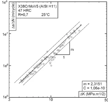
One characteristic curve forR¼ 0.7 is presented in Figure 7. The different values of constantsm and C of the Paris law[9] [Equation (4)], determined for all the experiments are summarized in Table 3.

Da=DN ¼ C:DKm ₍₄₎

Fig. 5. Crack modelling procedure.

Fig. 6. a) Wedge elements at the crack tip. b) Contour integral meshing.

Table 2. Conditions for crack propagation experiments.

Thickness [mm]

Applied stress Stress ratio R¼ smin/smax Test Frequency [Hz] Yield stress [%] 2.5 25/8.3 0.1 10 2.5 25 0.7 1.0 0.1 0.6 0.1

Fig. 7. Example of a Paris curve for R¼ 0.7.

Table 3. Paris law constants.

No. e [mm] R m C 1 2.5 0.1 2.39 0.72! 10%10 2 2.5 0.1 2.08 1.43! 10%10 3 2.5 0.7 2.04 2.62! 10%10 4 2.5 0.7 2.32 1.06! 10%10 5 0.6 0.1 2.18 1.07! 10%10

The slope of the propagation curves tends to increase approaching the threshold DKI. However, due to the large

dispersion in the data, the threshold values could not be clearly identified.

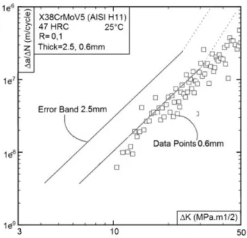
In Figure 8, a comparison is provided between the crack propagation rates atR¼ 0.1 and 0.7. It is evident that the crack propagation rate tends to increase with increasing R. Also compared are the propagation curves for thicknesses of 2.5 and 0.6 mm atR¼ 0.1 (Fig. 9). It can be seen that the data has a tendency to skew rightwards, i.e., there are reduced values of crack propagation rate for the same DKI.

Discussion

At 0.6 mm it seems that the testing condition approaches a plane stress condition. Detailed optical observations also reveal an important crack-tip plastic zone. In the 0.6 mm thickness specimen, the formation of patterns related to plastic deformation was also observed on the surface, which has not previously been observed on LCF experiments on this material on solid cylindrical specimens.[10,11] An effort was also made to measure the crack-tip opening displacement and crack closure in situ by optical measurements. At this stage, no clear crack closure could be demonstrated.

The difference in the crack propagation curves may be explained by two reasons. First, the KI, are calculated for a

plane-strain condition with small-scale yielding. In the experiments, these conditions do not strictly prevail. In particular, in the 0.6 mm specimen, the effect of the plane stress and large plastic zone has to be considered. The second explanation could be a different crack closure mechanism due to larger plastic deformations at the crack tip of the 0.6 mm specimen compared to the 2.5 mm specimen. More work has to be done on the stress state of the crack tip to have better insight into the difference in crack propagation curves. Conclusion

Crack propagation experiments are performed on SET specimens made of a hot-work martensitic tool steel, X38CrMoV5 (AISI H11). The effect of loading ratio R is studied. It is seen that the crack propagation rate increases with increasingR. The effect of thickness on propagation rate is also studied. A reduction in the crack propagation rates is observed with a reduction in specimen thickness.

[1] A. Persson, J. Bergstro¨m, C. Burman, in Proceedings of the 5thInternational Conference on Tooling 1999, pp. 167–177. [2] E. Ramous, A. Zambon, in Proceedings of the 5th

Inter-national Conference on Tooling 1999, pp. 179–184. [3] S. Hong, R. Weil,Thin Solid Films 1996, 283, 175. [4] R. Schwaiger, O. Kraft,Scr. Mater. 1999, 41, 823. [5] O. Kraft, R. Schwaiger, P. Wellner,Mater. Sci. Eng. 2001,

321, 919.

[6] S. Cravero, C. Ruggieri,Eng. Fract. Mech. 2007, 74, 2735. [7] M. S. Chiodo, S. Cravero, C. Ruggieri,Stress Intensity Factors for SE(T) Specimens, Technical Report BT-PNV-68, Faculty of Engineering, University of Sao Paulo 2006.

[8] R. John, B. Rigling,Eng. Fract. Mech. 1998, 60, 147. [9] P. C. Paris, F. Erdogan,J. Basic Eng. 1963, 85, 528. [10] D. Delagnes, PhD thesis, l’Ecole Nationale Supe´rieur des

Mines de Paris 1998.

[11] A. Oudin, PhD thesis, l’Ecole Nationale Supe´rieur des Mines de Paris 2001.