The massive survey. II. Stellar population trends out to large radius in massive early-type galaxies

(1)

Publisher’s version / Version de l'éditeur:

Vous avez des questions? Nous pouvons vous aider. Pour communiquer directement avec un auteur, consultez la

première page de la revue dans laquelle son article a été publié afin de trouver ses coordonnées. Si vous n’arrivez pas à les repérer, communiquez avec nous à [email protected].

Questions? Contact the NRC Publications Archive team at

[email protected]. If you wish to email the authors directly, please see the first page of the publication for their contact information.

https://publications-cnrc.canada.ca/fra/droits

L’accès à ce site Web et l’utilisation de son contenu sont assujettis aux conditions présentées dans le site LISEZ CES CONDITIONS ATTENTIVEMENT AVANT D’UTILISER CE SITE WEB.

The Astrophysical Journal, 807, 1, 2015-06-24

READ THESE TERMS AND CONDITIONS CAREFULLY BEFORE USING THIS WEBSITE.

https://nrc-publications.canada.ca/eng/copyright

NRC Publications Archive Record / Notice des Archives des publications du CNRC :

https://nrc-publications.canada.ca/eng/view/object/?id=1ce254a0-05bc-48a0-bf42-b1721a3b778d

https://publications-cnrc.canada.ca/fra/voir/objet/?id=1ce254a0-05bc-48a0-bf42-b1721a3b778d

NRC Publications Archive

Archives des publications du CNRC

This publication could be one of several versions: author’s original, accepted manuscript or the publisher’s version. / La version de cette publication peut être l’une des suivantes : la version prépublication de l’auteur, la version acceptée du manuscrit ou la version de l’éditeur.

For the publisher’s version, please access the DOI link below./ Pour consulter la version de l’éditeur, utilisez le lien DOI ci-dessous.

https://doi.org/10.1088/0004-637X/807/1/11

Access and use of this website and the material on it are subject to the Terms and Conditions set forth at

The massive survey. II. Stellar population trends out to large radius in

massive early-type galaxies

Greene, Jenny E.; Janish, Ryan; Ma, Chung-Pei; McConnell, Nicholas J.;

Blakeslee, John P.; Thomas, Jens; Murphy, Jeremy D.

(2)

THE MASSIVE SURVEY. II. STELLAR POPULATION TRENDS OUT TO

LARGE RADIUS IN MASSIVE EARLY-TYPE GALAXIES

Jenny E. Greene1, Ryan Janish2, Chung-Pei Ma3, Nicholas J. McConnell4, John P. Blakeslee5,

Jens Thomas6, and Jeremy D. Murphy7

1_{Department of Astrophysics, Princeton University, Princeton, NJ 08544, USA} 2_{Department of Physics, University of California, Berkeley, CA 94720, USA} 3_{Department of Astronomy, University of California, Berkeley, CA 94720, USA} 4_{Institute for Astronomy, University of Hawaii at Manoa, Honolulu, HI 96822, USA}

5_{Dominion Astrophysical Observatory, NRC Herzberg Institute of Astrophysics, Victoria, BC V9E 2E7, Canada} 6_{Max Planck-Institute for Extraterrestrial Physics, Giessenbachstr. 1, D-85741 Garching, Germany}

7_{IXL Learning, 777 Mariners Island Blvd., Suite 600, San Mateo, CA 94404}

Received 2015 February 24; accepted 2015 April 27; published 2015 June 24

ABSTRACT

We examine stellar population gradients in ∼100 massive early-type galaxies spanning180 <s_*<370km s−1and

MKof−22.5 to −26.5 mag, observed as part of the MASSIVE survey. Using integral-ﬁeld spectroscopy from the

Mitchell Spectrograph on the 2.7 m telescope at McDonald Observatory, we create stacked spectra as a function of radius for galaxies binned by their stellar velocity dispersion, stellar mass, and group richness. With excellent sampling at the highest stellar mass, we examine radial trends in stellar population properties extending to beyond

twice the effective radius (~_2.5R_e_{). Speciﬁcally, we examine trends in age, metallicity, and abundance ratios of}

Mg, C, N, and Ca, and discuss the implications for star formation histories and elemental yields. At a ﬁxed physical radius of 3–6 kpc (the likely size of the galaxy cores formed at high redshift), stellar age and [α/Fe] increase with

increasings and depend only weakly on stellar mass, as we might expect if denser galaxies form their central_*

cores earlier and faster. If we instead focus on_1–1.5R_e, the trends in abundance and abundance ratio are washed

out, as might be expected if the stars at large radius were accreted by smaller galaxies. Finally, we show that when

controlling fors , there are only very subtle differences in stellar population properties or gradients as a function of_*

group richness; even at large radius, internal properties matter more than environment in determining star formation history.

Key words:galaxies: elliptical and lenticular, cD – galaxies: evolution – galaxies: kinematics and dynamics – galaxies: stellar content

1. INTRODUCTION

The assembly history of elliptical galaxies remains a major unsolved problem for galaxy evolution. Recent observations point to dramatic size evolution of the most massive galaxies

from z ≈ 2 to the present (e.g., van Dokkum et al.2008; van

der Wel et al.2008; Patel et al.2013; van der Wel et al.2014).

The extent to which these trends require late-stage minor

mergers (e.g., Oser et al. 2012) or can be explained by the

addition of larger, younger galaxies at later times (Valentinuzzi

et al.2010; Newman et al.2012; Barro et al.2013) remains a

topic of ongoing debate. Information lurking in the faint outer parts of present-day massive ellipticals can complement high-redshift measurements. Radial gradients in stellar populations distinguish when and how the stars at large radius were formed

(e.g., White 1980; Kobayashi 2004; Greene et al. 2013;

Hirschmann et al.2015), while the kinematics of the stars (e.g.,

V *

s , the level of radial anisotropy, etc.) contain clues about

how these stars entered the halo (e.g., Arnold et al.2014; Naab

et al. 2014; Raskutti et al. 2014; Röttgers et al. 2014; Wu

et al.2014).

Here we focus on the average radial trends in stellar populations of early-type galaxies using our ambitious survey of the hundred most MASSIVE galaxies within 100 Mpc (Ma

et al.2014). Observations of the stellar populations in elliptical

galaxy outskirts are challenging, since their surface bright-nesses drop steeply with radius. Despite more than thirty years of effort, most observations of stellar population gradients do

not extend much beyond the half-light radius (Spinrad &

Taylor 1971; Faber et al. 1977; Gorgas et al. 1990; Fisher

et al.1995; Kobayashi & Arimoto1999; Ogando et al. 2005;

Brough et al. 2007; Baes et al. 2007; Annibali et al. 2007;

Sánchez-Blázquez et al.2007; Rawle et al. 2008; Kuntschner

et al. 2010; McDermid et al. 2015; Oliva-Altamirano

et al. 2015). Resolved stellar population studies have

uncovered a low-metallicity halo component at very large radius, but only in a handful of nearby galaxies (e.g., Kalirai

et al. 2006; Harris et al. 1999; Rejkuba et al. 2005; Harris

et al. 2007; Crnojević et al. 2013; Pastorello et al. 2014;

Peacock et al.2015; Williams et al.2015). There are also a few

long-slit observations that extend to large radius (Carollo

et al. 1993; Carollo & Danziger 1994; Mehlert et al. 2003;

Kelson et al. 2006; Spolaor et al.2010; Pu et al.2010; Pu &

Han2011). Even integral-ﬁeld spectrographs, now widely used

for the study of spatially resolved galaxy properties (Emsellem

et al. 2004; Cappellari et al. 2006, 2012; Sarzi et al. 2006),

include few observations that extend beyond the half-light

radius in integrated light (Weijmans et al. 2009; Murphy

et al.2011).

The ∼100 galaxies analyzed here represent a signiﬁcant improvement over previous work. Using coadded spectra as a function of radius, we will investigate whether radial gradients depend not only on stellar velocity dispersion, but also on other intrinsic galaxy properties such as stellar mass and

environ-mental density. We ﬁnd a hint that at ﬁxeds , galaxies residing_*

in higher densities are older and more α-element enhanced, but

(3)

we see no evidence for differing gradients for galaxies in low and high densities.

We present the sample in Section 2, the observations and

data reduction in Section 3, our stellar population analysis in

Section 4, and the radial variations in stellar populations in

Section 5. We summarize our ﬁndings and conclude in

Section 6. Throughout we assume a concordance cosmology

with H0=70km s−1Mpc−1,W =M 0.3, andW =L 0.7

(Dunk-ley et al.2009).

2. SAMPLE

The MASSIVE sample selection is described in detail in Ma

et al. (2014). For completeness, we summarize the sample

selection brieﬂy here. MASSIVE is a volume-limited sample of the 116 most massive galaxies within 108 Mpc. The galaxies are selected from the 2MASS Redshift Survey (Huchra

et al. 2012), using a total K-band magnitude limit of

MK< -_25.3mag (roughly 1011.5M). Using the Hyperleda

database (Paturel et al.2003), we apply a morphological cut to

remove large spiral and interacting galaxies. The resulting 116 galaxies span a wide range of stellar velocity dispersion

(∼180–400 km s−1_{) and, based on the group catalog of Crook}

et al. (2007), are found in a wide array of environments, from

“ﬁeld” galaxies with no ~L* companions to rich clusters

(Coma, Perseus, and Virgo). In this paper, we include 49

MASSIVE galaxies with large-format integral-ﬁeld

spectrograph observations in hand. While we are also obtaining high spatial resolution integral ﬁeld spectroscopy for a subset of galaxies for black hole mass determinations (e.g.,

McCon-nell et al. 2012), this paper deals exclusively with the

Mitchell data.

In addition to the ongoing MASSIVE survey, we include

here a sample of lower-mass galaxies (Greene et al. 2013)

selected directly from the Sloan Digital Sky Survey (SDSS;

York et al.2000) and observed with an identical set-up with the

Mitchell Spectrograph. As the selection was different, we

brieﬂy review it here (see also Greene et al. 2012; Raskutti

et al. 2014). Since the spectral resolution of the Mitchell

Spectrograph is sinst»150km s−1 at 4000 Å, we select

galaxies with dispersion measurements from the SDSS that

are greater than this value. Individual ﬁbers are 4. 2 in

diameter, and so we aim for galaxies with effective radii at least twice as large. Galaxies with distances of 40–95 Mpc are large enough to be well-resolved but small enough to ﬁt into one

pointing. We use a color selection of u- >r _2.2 _(Strateva

et al. 2001), which preferentially selects early-type galaxies,

and then remove the few edge-on disk galaxies by hand, but keep S0 galaxies. These 46 galaxies are of uniformly lower stellar mass than those in MASSIVE. Taken together, the

sample galaxies span a range of -_22.5<MK < -_26.5

Vega mag. The sample properties for the 95 galaxies (49 from

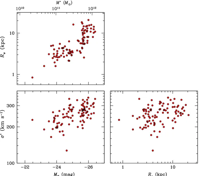
MASSIVE) are summarized in Figure1.

3. OBSERVATIONS AND DATA REDUCTION The majority of the galaxies presented here were observed over ten observing runs between 2011 September and 2014 April. There are an additional four galaxies taken earlier as part

of the PhD thesis of Jeremy Murphy (Murphy et al.2011) and

four taken by Nicholas McConnell (McConnell et al. 2012).

All of these data were taken with the George and Cynthia Mitchell Spectrograph (the Mitchell Spectrograph, formerly

VIRUS-P; Hill et al. 2008) on the 2.7 m Harlan J. Smith

telescope at McDonald Observatory. The Mitchell

Spectrograph is an integral-ﬁeld spectrograph with 246 ﬁbers

subtending 4. 2 each and covering a 107″ × 107″ ﬁeld of view

with a one-third ﬁlling factor. As such, the Mitchell Spectrograph is ideal for studying the low surface brightness

outer parts of nearby galaxies (Blanc et al. 2009; Yoachim

et al.2010; Murphy et al.2011; Adams et al.2012).

We utilize the blue setting of the Mitchell spectrograph with a resolution of R ≈ 850 and spanning a wavelength range of 3550–5850 Å. This resolution (roughly a FWHM of 5 Å)

delivers a dispersion of ∼1.1 Å pixel−1and corresponds to

* s ≈

150 km s−1at 4300 Å, our bluest Lick index, improving to

∼100 km s−1at the red end of the spectrum. Each galaxy was

observed for a total of ∼2 hr on source with one-third of the time spent at each of three dither positions to ﬁll the ﬁeld of view. Observations are interleaved with sky observations of 10 min duration. Initial data reduction is accomplished using

the custom code Vaccine (Adams et al. 2011; Murphy

et al. 2011). The details of our data reduction are described

in Murphy et al. (2011), so we repeat only a brief overview for

completeness here.

We first perform overscan and bias subtraction for all science and calibration frames. The fiber trace is determined from the twilight flats, taking into account curvature in the spatial

direction and following the techniques of Kelson (2003) to

avoid interpolation and thus correlated errors. Arcs are used to derive a wavelength solution with typical rms residual variations about this best-fit fourth-order polynomial between 0.05 and 0.1 Å. The twilight flats are also used to construct the flat field, once the solar spectrum has been modeled and

removed. The ﬂat ﬁeld is typically stable to 0.1< pixels for

typical thermal variations in the instrument. The flat field is then applied to all of the science frames to correct variations in the pixel-to-pixel responses, as well as the relative fiber-to-fiber variation, and the cross-dispersion profile shape for every fiber. The sky is modeled using off-galaxy sky frames observed with a sky-object-object-sky pattern. The sky frames are processed in the same manner as the science frames. In general, each sky nod is weighted equally, except for very cloudy conditions. Finally, cosmic rays are identified and masked.

We use software developed for the VENGA project (Blanc

et al.2009,2013) for ﬂux calibration and ﬁnal processing. We

observe flux calibration stars using a six-point dither pattern and derive a relative flux calibration in the standard way. We can test the wavelength dependence of the flux calibration by comparing the shape of the spectrum in the central fiber of the Mitchell Spectrograph with the SDSS spectrum for those galaxies with SDSS spectra. We find 10% disagreement in nearly all cases, with no more than ∼15% differences at worst. We then correct the default astrometric solutions using photometry, by deriving an astrometric match between each

image and an SDSS (York et al. 2000) or PanSTARRS

(Schlaﬂy et al.2012; Tonry et al.2012; Magnier et al.2013)

image. Finally, all ﬁbers are interpolated onto the same wavelength scale and combined into radial bins.

3.1. Effective Radii

In our previous work, we adopted the SDSS model radius (the

de Vaucouleurs ﬁt) as the effective radius (Re). While there is

considerable evidence that the shape of the light proﬁle changes

systematically with galaxy mass (e.g., Caon et al. 1993;

2

(4)

Ferrarese et al.2006; Kormendy et al.2009), fitting the galaxies with a fixed Sérsic index of four has the benefit that we are less sensitive to both sky subtraction errors (Mandelbaum

et al. 2005; Bernardi et al.2007) and to the detailed shape of

the light proﬁle in the very faint wings (e.g., Lackner &

Gunn2012). In the case of MASSIVE, ∼1/3 of the galaxies do

not have SDSS imaging, so we adapt a size measurement from

2MASS (Jarrett et al.2003). We use the median effective radius

measured from the JHK band (see Equation (3) in Ma

et al. 2014). The 2MASS size measurement tends to

under-estimate the galaxy sizes relative to the SDSS (Lauer et al.2007;

Kormendy et al.2009). To put the size measurements on equal

footing, Ma et al. (2014) ﬁt a linear conversion between R2MASS

and RSDSS: log (R10 2MASS)=0.8 log (R10 SDSS)-0.076 (their

Equation (4)). We use this relation to correct the 2MASS measurements to match the SDSS measurements.

3.2. Radial Bins

Spectra from individual ﬁbers, with the exception of those at the very center of the IFU, have inadequate signal for stellar population studies. Therefore, all of our analysis is performed on binned spectra. We utilize two binning schemes here, in

both cases deﬁning elliptical annuli based on the axis ratio measured by the SDSS or 2MASS. Since galaxies get larger as

they get more massive, we make bins of width _0.5R_e.

However, it is also interesting to look at trends as a function of physical size, and here we extend from 0–15 kpc in 3 kpc increments. For the physical bins, we use the central ﬁber as the central bin; while this central ﬁber corresponds to a different physical size for each system, it provides our highest spatial resolution bin.

3.3. Stellar Velocity Dispersion Measurements Stellar velocity dispersions are required for measuring Lick indices. This is because at ﬁxed intrinsic absorption, as the velocity dispersion increases, the measured equivalent width (EW) decreases. Thus, a correction must be applied to put all indices on the same scale. We also use the central stellar velocity dispersions to rank galaxies in constructing coadded

spectra. Our central 4. 2 ﬁber is similar to the SDSS ﬁber and

thus easily compared with the literature. We use pPXF to

measure the dispersions (Cappellari & Emsellem 2004). We

compare ours measurements with SDSS measurements when_*

available or our compiled literature values (Ma et al. 2014)

Figure 1.Distributions of basic structural properties for our sample. On bottom left, stellar velocity dispersion (s ) measured within the central ﬁber is plotted against_* MK(mag; total magnitude) from 2MASS. On top left, we show effective radius, from the NSA catalog (or from 2MASS with a correction; Section3.2) against MK

and on bottom right effective radius vs. stellar velocity dispersion.

3

(5)

derived from the Hyperleda database (Paturel et al.2003). We

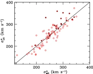
ﬁnd very good agreement, with the median (sMS-sLit)/

0.01 0.09

Lit

s =  . That is, we see no systematic offset

between the two sets of measurements and a scatter of 9%.

We compare our measurements with the literature in Figure2.

As discussed in van den Bosch et al. (2015), there is some

excess scatter at the high dispersion end, speciﬁcally when we compare with Hyperleda. However, we ﬁnd better agreement with Hyperleda than reported by van den Bosch et al. predominantly due to recent (post-2013) changes in Hyperleda. We have 51 objects in common with the van den Bosch HET

catalog, and we also ﬁnd reasonable agreement with theirs_*

measurements, with (sMS-sHET) sHET= -0.030.07.

Throughout, s refers to our measurements from the central_*

ﬁber unless otherwise speciﬁed.

4. ANALYSIS

4.1. Stellar Population Modeling Approach

We use Lick indices as a tool to trace the stellar populations. Lick indices were developed as a way to extract stellar population information from spectra without ﬂux calibration, but still circumvent classic age–metallicity degeneracies

(Bur-stein 1985; Faber et al. 1985; Worthey et al. 1992; Trager

et al.1998). The Lick indices are narrow regions of the spectra

(typically ∼20 Å wide) that are dominated by a single element and thus are predominantly sensitive to orthogonal aspects of the stellar population properties; Hβ is sensitive to age, Fe indices to [Fe/H], and so on. It is important to bear in mind that at the

velocity dispersion of our target galaxies (200–400 km s−1_{) all}

indices are blends of multiple elements. See, for example, Table

1 in Graves & Schiavon (2008) for the primary elements that

dominate the Lick indices used in this work.

Lick indices are still widely used in the literature as they mitigate difﬁculties in modeling the effects of abundance ratio

changes (e.g., Worthey et al. 1994; Gallazzi et al. 2005).

Trager et al. (2000b, 2000a) developed a technique to derive

index responses from stellar atmosphere models, such that even if the full spectrum cannot be calculated, the index EW changes due to changing abundance ratios can be incorporated into an analysis of line EWs. On the other hand, the current generation

of full spectral synthesis codes are very sophisticated (e.g.,

Vazdekis et al.2010; Conroy & van Dokkum2012) and have

been designed to ﬁt non-solar abundance ratios.

For reference, we review the main indices that we use to derive the basic stellar population parameters. The reader is

referred to Graves & Schiavon (2008) for more detailed

information. We use lick_ew (Graves & Schiavon 2008) to

measure the Lick indices and the stellar population modeling

code EZ_Ages (Graves & Schiavon2008) to convert the Lick

indices to physical parameters (age, [Fe/H], [α/Fe]). The code

works on a hierarchy of index pairs, starting with Hβ and Feá ñ,

and iteratively solves for the age, abundance and abundance

ratios. The models of Schiavon (2007) include abundance ratio

differences using the response functions of Korn et al. (2005).

For a different inversion methodology see Thomas et al. (2011)

or for full spectral ﬁtting comparisons see Conroy et al. (2014).

As emphasized by Schiavon (2007), because we do not

directly measure the oxygen abundance and oxygen is the most abundant heavy element, it is misleading to quote total metallicity. Instead, we quote [Fe/H], which is directly inferred from the Fe indices. If we assume that [O/Fe] tracks [Mg/Fe], then we can use the latter to infer [Z/H]. We will generally assume that O and Mg follow similar trends as they are both

αelements, and thus use [Mg/Fe] interchangeably with [α/Fe].

Based on the same assumption, we also will use the conversion

from Trager et al. (2000b): [Z/H] = [Fe/H] + 0.94[α/Fe] to

calculate the metallicity. For alternate approaches to modeling

oxygen using Lick indices, see Johansson et al. (2012) or

Worthey et al. (2014). In our default runs, we utilize the

α-enhanced isochrone from Salasnich et al. (2000) and the

default assumption that [O/Fe] = 0.5 to match the α-enhanced isochrone value.

Carbon is roughly half as abundant by number as oxygen at

solar abundances (Asplund et al.2009). We derive [C/Fe] from

the C24668index (e.g., Tripicco & Bell1995; Trager et al.1998;

Graves et al.2007; Johansson et al.2012). Because the amount

of C locked into CO depends on the oxygen abundance, as we lower the assumed O abundance, the inferred C abundance

drops commensurately (Serven et al. 2005). We will quantify

the magnitude of this effect below.

Nitrogen (one-tenth the O abundance by number in the Sun) is then derived from CN1 (4143–4178 Å) once we have a C

abundance. As discussed in Greene et al. (2013), there are

some uncertainties associated with CN due to the low signal-to-noise ratio (S/N) at the blue end of the spectrum, but our nuclear CN measurements match those from the SDSS spectra of the same galaxies (our Mitchell indices are 0.01 ± 0.02 mag lower than the SDSS measurements), giving us some conﬁdence in these measurements.

Finally, the Ca abundance (one-hundredth the C abundance by number in the Sun) is based on the Ca4227 index

(4223.5–4236.0 Å; Worthey1998). This index is blended with

CN, and thus the [Ca/Fe] measurement is most uncertain, as it is dependent on both the [C/Fe] and [N/Fe] measurements.

Others have used Ca H + K (Serven et al. 2005; Worthey

et al.2014) or the Ca Triplet at 8600 Å, where the last is also

sensitive to the dwarf-to-giant ratio (e.g., Cenarro et al.2004).

Since the Lick indices are very sensitive to small errors in sky subtraction and other small-scale errors, we construct stacked spectra and measure the average radial trends in the Lick indices and resulting stellar populations.

Figure 2. Stellar velocity dispersions (s ) measured within the central 4. 2_*  Mitchell ﬁber are compared with literature values. Open symbols have literature measurements from the SDSS, while ﬁlled symbols are from Hyperleda. The overall agreement is quite good, with (s_*MS-s_*Lit_{) *}sLit= 0.01 ± 0.09.

4

(6)

4.2. Equivalent Widths and Emission Line Corrections There are a number of systematic effects that may impact the EWs. One relates to the velocity dispersion: while the default dispersion corrections within lick_ew were veriﬁed originally

over the range s =_* 250–300km s−1, some of our galaxies

exhibit even larger s . We therefore check our dispersion_*

corrections using simple stellar population models from

(Conroy & van Dokkum 2012), broadened over the full

observed range ofs . The Lick indices that we recover using_*

the default lick_ew corrections agree with the input values within 0.02 Å for an α-enhanced model with a Salpeter IMF, which is a good approximation to our galaxies. The corrections are a weak function of stellar population parameters, but only at the hundredths of an Å level, which is small compared to our other sources of systematic error.

A larger correction must be made for low-level emission that can ﬁll in the absorption lines and artiﬁcially lower their EWs. Weak emission from warm ionized gas is very common in the

centers of elliptical galaxies (Sarzi et al. 2010; Yan &

Blanton 2012), and small amounts of line inﬁll can lead to

signiﬁcant errors in recovered parameters. Even 0.1 Å errors in Hβ EW can lead to errors of ∼1–2 Gyr in the modeling (e.g.,

Schiavon 2007).

Given the very low emission levels and the large uncertainties involved, we compare two methods for

determin-ing the levels of [OIII] and Hβ emission. In Greene et al.

(2012), we utilized pPXF+GANDALF developed by M. Sarzi

(Sarzi et al. 2006) and M. Cappellari (Cappellari &

Emsellem2004) to simultaneously model the stellar absorption

and emission lines. GANDALF is very robust for well-detected lines, but under-constrained for very weak emission. Following

Greene et al. (2013), we also ﬁt each spectrum with an

empirical template drawn from the composite spectra of Graves

et al. (2010). We then ﬁt the [OIII] emission in the residual

spectrum, and subtract both [OIII] and Hβ, assuming that the

Hβ emission is 70% of the [OIII_{] ﬂux (measured to within a}

factor of two, Trager et al.2000b; Graves et al.2007). We then

iterate these ﬁts until the emission line ﬂux has converged. In addition, we search for residuals around strong sky lines at 5200 and 5460 Å.

From our iterative fits, and focused on the galaxy centers for simplicity, roughly two-thirds of the galaxies have low-level Hβ emission detected, with a median EW of 0.2 Å, and a maximum of 1 Å (calculated for those galaxies with detected Hβ). The Gandalf measurements do not correlate very strongly with our iterative fits. In the GANDALF fits, only half of the galaxies have detections, with a median EW is 0.2 Å and a maximum Hβ EW of 1.7 Å. As a means of quantifying our systematic errors, we rerun the stacking analysis described below on the Gandalf-subtracted spectra. As expected, only the stellar age changes significantly, being ∼3 Gyr lower in the Gandalf stacks. But all other stellar population properties are virtually identical (with the [Fe/H] shifting higher by a small amount to compensate the shift in stellar age). Thus, we present results based on the iterative fits, but we caution that there is a rather large systematic uncertainty in the absolute stellar age. All other stellar population properties are robust to this modeling difficulty, and in general the relative ages are robust as well. We are currently working on more robust gas detection schemes using all lines in the spectra (V. Pandya et al. 2015, in preparation).

We then use lick_ew (Graves & Schiavon 2008) on the

emission-line corrected spectra. The indices are on a modiﬁed

Lick system presented by Schiavon (2007) based on

ﬂux-calibrated spectra. In order to demonstrate that we are on the same system, we compare the Lick indices from the ﬂux-calibrated SDSS spectra (the inner 3″) with those from

the central 4. 2 ﬁber in our data. There is no net offset

between the two sets of indices in any case, with

(Hb EWS Hb EW ) HMS bEWMS

á - ñ = 0.080.17, where

S is SDSS and MS is the Mitchell Spectrograph. Feá ñ and

Mgb each have a scatter of only ∼10% and even smaller net offsets.

4.3. Composite Spectra

While measuring Lick indices is a very powerful technique for high S/N spectra, at the large radii that we are working, systematic effects such as small errors in sky subtraction and ﬂux calibration can begin to cause large uncertainties in the Lick indices measured from individual objects. Stacked spectra average over sky subtraction and ﬂux calibration errors in individual systems, which occur at different wavelengths in

each galaxy rest-frame (e.g., Graves et al.2009; Yan2011). Of

course, variations in stellar populations at a givens or mass_*

are expected based on differences in accretion history (e.g.,

Hirschmann et al. 2015) and we are quite interested in these

differences, particularly as a function of the dynamical properties of the galaxies. We plan to implement full spectral ﬁtting in the near future, which is more robust at low S/N (e.g.,

Choi et al.2014).

We know that stellar population properties are a strong

function ofs (e.g., Worthey et al._* 1992; Bender et al. 1993;

Trager et al.2000a; Graves et al.2009). Thus, we ﬁrst divide the

galaxies into four stellar velocity dispersion bins using our pPXF measurements to the central ﬁber. Of the 95 galaxies in our sample, we exclude eight. Most of these are from the low-mass sample and have a bright star in the foreground making it difﬁcult to reach a reasonable S/N. NGC1167 in the MASSIVE sample is excluded because it may be a face-on disk galaxy. We will treat it more carefully in future work. The bins have

*

s < 220 km s−1_{(15 objects), 220 <} *

s < 250 km s−1₍₂₁

objects), 250 < s < 290 km s_* −1_{(33 objects), and all those}

higher thans > 290 km s_* −1_{(18 objects). Stacked spectra within}

R

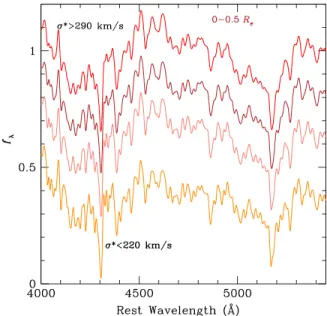
0.5 e are shown in Figure3. The resulting stellar population

parameters are shown in Figure4. We reach different physical

radii for different bins as we run out of signal for the smaller and lower-mass galaxies. Also, the total number of galaxies included in the largest radial bin is typically ∼30% smaller than the centers, as various systematic effects such as foreground star contamination grow more severe at low ﬂux levels.

Below, we will also bin on stellar mass and group richness. While the detailed bins are different, the stacking technique described here is the same for these different sets of bins.

To create the stack, we coadd the emission-line–subtracted spectra. We interpolate the rest-frame spectra onto a common wavelength grid. To ensure we know the dispersion of the ﬁnal stacked spectrum, we then smooth each galaxy to a value that is

30% higher than the uppers limit of each bin. This smoothing_*

ensures that all galaxies go into the stack with the same effective dispersion. With this approach, we minimize small errors due to dispersion corrections to the Lick indices. An alternate procedure would be to smooth all templates, in all

bins, to a high dispersion (e.g., 400 km s−1_{). We ﬁnd very small}

5

(7)

(<0.01 Å) differences in the resulting indices if we adopt the latter approach, again conﬁrming that our dispersion

correc-tions are working (Section 4.2). When we make bins in MK

below, because of the wide range ofs in each bin, we smooth_*

all bins to 400 km s−1.

We remove the continuum by dividing each spectrum by a heavily smoothed version of itself. This step simultaneously normalizes all spectra to the same level and ensures that differences in continuum shape (whether real or due to small errors in sky subtraction or flux calibration) do not impact the final line strengths. We then calculate the median flux at each pixel, with rejection, although we get very similar results using

the biweight estimator (Beers et al.1990). We experiment with

multiplying the coadded spectrum by the median continuum before measuring indices, but the changes to the Lick indices are negligible.

4.4. Uncertainties

To determine the level of variation in the composite spectra, we generate 100 boot-strapped composite spectra by randomly drawing from the total list of galaxies in that bin, with replacement. We measure Lick indices from each of these 100 trial spectra. We then assign errors on the Lick indices that enclose 68% of the Lick indices measured from the 100 trials. Therefore, the size of the error is most directly related to the variance in parameters over the population in that bin, rather than measurement or modeling uncertainty. The systematic uncertainties are not shown. Age measurements have large

systematic uncertainties due to emission inﬁll (Section 4.2),

while nitrogen and calcium are particularly uncertain due to their dependence on blue spectral features and assumed carbon and oxygen abundances.

In general, we report the measurement from the primary stacked spectrum, and the errors derived from the boot-strapped spectra. There are a few cases where the Lick index measured from the primary stacked spectrum does not fall within the

stellar population grids (usually because the Hβ index is slightly too low). In these cases, we use the median index value from the 100 trials as the ﬁnal answer. These cases are indicated with open symbols.

5. RADIAL VARIATIONS IN STELLAR POPULATIONS 5.1. Bins of σ*

In Figure 4 we show radial trends in the measured age,

[Fe/H], and abundance ratios as a function of physical (left) and

Re-scaled (right) radii. Our default models make the

assump-tion that [O/Fe] is enhanced like [Mg/Fe], since they are both

αelements. However, in Figure4we indicate with dashed lines

the C, N, and Ca abundances that result for an assumed solar [O/Fe]. While the zeropoints of [C/Fe] and [N/Fe] both decline, the radial trends will not change unless [O/Fe] (unlike [Mg/Fe]) changes with radius.

We fit a power-law relation between radius and each stellar population property. We anchor the relation at the center of our radial coverage. Eventually, when we have reliable K-band light profiles for each galaxy, we will calculate mass-weighted stellar population properties, but at present, for a given stellar population property X we fit a log-linear relationship :

X=A _log(R R₃₎+ , where R_B ₃is the third bin,

correspond-ing either to 3–6 kpc or_1–1.5R_e. The quantity A represents the

radial gradient per log radius. The quantity B represents an effective stellar population property at the center of our radial coverage. The ﬁts to A and B for each relation are shown in

Tables1 and2.

The strongest radial gradients are found between [Fe/H] and [C/Fe], which both decline with radius. Age shows a decline in the highest dispersion bin, but because that effect is weaker when we use the alternate emission line correction, we treat age gradients with extra caution. All other abundance ratios measured here are consistent with remaining ﬂat over the full radial range, aside from a 2σ increase in [Ca/Fe] at large radius

that is only seen in the largests bin._*

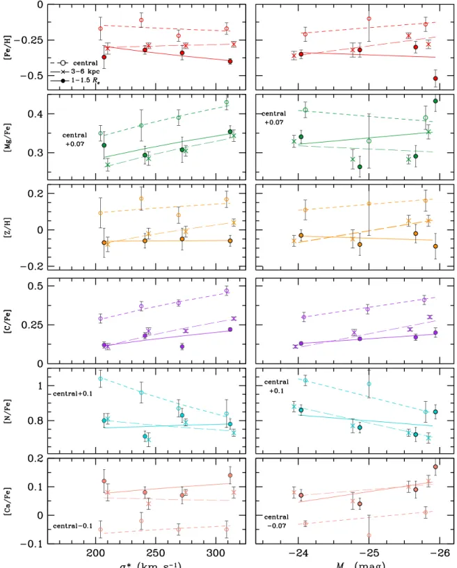
We turn to trends between stellar populations ands . Our_*

central bins are shown as open circles in Figure5. We recover

well-known trends between stellar population properties and stellar velocity dispersion for galaxy centers. Galaxies with higher stellar velocity dispersions have older stellar ages and

higher [Mg/Fe] and [C/Fe] ratios (e.g., Trager et al. 2000b;

Worthey 2004; Thomas et al. 2005; Sánchez-Blázquez

et al. 2006; Graves et al. 2007; Smith et al. 2009; Price

et al.2011; Johansson et al.2012; Conroy et al.2014; Worthey

et al.2014). One interesting exception is [N/Fe], where we see

a decline with s . This trend is at odds with our previous_*

ﬁnding (Greene et al.2013), as well as most other work on the

topic (although see also Kelson et al. 2006). More detailed

work is needed to conﬁrm this trend, particularly given possible uncertainties in ﬂux calibration in the blue for the Mitchell spectra. Recall also that the very old ages found in the very centers of these galaxies have 2–3 Gyr error bars, and thus are consistent with the age of the universe.

Thanks to our spatial coverage, we can go beyond the trends

between s and stellar populations in the galaxy center, and_*

look at how these trends evolve as we look to larger radius,

both in physical and R scalede‐ units. The crosses in Figure5

show the trends betweens and stellar population properties_*

measured at 3–6 kpc. In general, the same trends are seen with *

s in the central and 3–6 kpc bins ([N/Fe] is again an

Figure 3.Coadded spectra within0.5Re, for stellar velocity dispersion stacks starting from s < 220 km s_* −1_{(bottom) to}

*

s > 290 km s−1_{(top). Each}

spectrum has been normalized to unity as described in the text, and the ﬂux density offsets are arbitrarily applied for display purposes. In creating the stacks, each galaxy was smoothed to a value 30% more than the upper end of the dispersion range in creating the stack.

6

(8)

exception). Fit values are included in Table3. [C/Fe] shows the

most signiﬁcant correlation with s , with a positive slope_*

detected at 8s signiﬁcance. We ﬁnd a weak trend with [α/Fe]

(3.5σ) and a strong trend with age (7σ; not shown). The

measured slopes betweens and [Fe/H], [Ca/Fe], and [N/Fe] are_*

all consistent with zero; that is, the effective value of these

parameters is similar for alls bins._*

We can also evaluate trends between s and stellar_*

population properties evaluated beyond Re(taken here to be the

R

1–1.5 e bin). In this case, the physical radii increase for the

higher-dispersion bins. Interestingly, we ﬁnd that the trends withs are weaker when evaluated as a function of R_* e. Only stellar age (7σ) and [C/Fe] (much more weakly at 4σ) correlate

positively with s . Apparently, trends between_* s and_*

abundance ratios are strongest when measured within small physical radii. If galaxies indeed form a compact core rapidly at high redshift, then we expect this inner region (<5 kpc; e.g.,

van der Wel et al.2014_{) to depend most strongly on *}s .

Before we interpret these observed trends in more detail, we

examine differences between bins ins and stellar mass._*

5.2. Bins of M*

There is now a preponderance of evidence that stellar

population properties correlate most strongly with s at their_*

centers (Bender et al. 1993; Trager et al. 2000b; Graves

et al.2009; Wake et al. 2012). However, there is little work

Figure 4.Radial gradients in age, [Fe/H], [Mg/Fe], [C/Fe], [N/Fe], and [Ca/Fe] as calculated by EZ_Ages from the Lick indices measured in the coadded spectra. The measurements are made on four stacked spectra binned on stellar velocity dispersion (see Figure key), and are shown as a function of R in kpc (left) or R Re. We ﬁt the radial gradients with a power law of the form X=A log(R R3)+Bfor each stellar population parameter X, where R3is either 3–6 kpc or1–1.5Re. The ﬁts to the

highest (long-dashed lines) and lowest dispersion (dotted lines) are shown here, and in Tables1and2. Note the decline with radius in [Fe/H] and [C/Fe] in contrast with the radially constant age, [Mg/Fe], [N/Fe], and [Ca/Fe]. To indicate systematic errors in the light elements due to the unknown oxygen abundance, we also show the resulting models assuming [O/Fe] = 0.1 rather than the default [O/Fe] = 0.5 (keeping [O/Fe] constant with radius in both cases;s > 290 km s_* −1and 220 <

*

s

< 250 km s−1are shown in colors that match the symbol). The [C/Fe] lines with alternate oxygen abundance have been offset by

−0.1 dex for presentation purposes.

7

(9)

Table 1 Gradient Fits (Re)

Stack Aage Bage A[Fe/H] B[Fe/H] A[α/Fe] B[α/Fe] A[C/Fe] B[C/Fe] A[N/Fe] B[N/Fe] A[Ca/Fe] B[Ca/Fe]

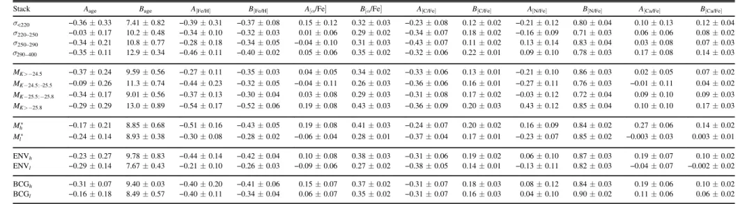
σ<220 −0.36 ± 0.33 7.41 ± 0.82 −0.39 ± 0.31 −0.37 ± 0.08 0.15 ± 0.12 0.32 ± 0.03 −0.23 ± 0.08 0.12 ± 0.02 −0.21 ± 0.12 0.80 ± 0.04 0.10 ± 0.13 0.12 ± 0.04 σ220–250 −0.03 ± 0.17 10.2 ± 0.48 −0.34 ± 0.10 −0.32 ± 0.03 0.01 ± 0.06 0.29 ± 0.02 −0.34 ± 0.07 0.18 ± 0.02 −0.16 ± 0.09 0.71 ± 0.03 0.06 ± 0.06 0.08 ± 0.02 σ250–290 −0.34 ± 0.21 10.8 ± 0.77 −0.28 ± 0.18 −0.34 ± 0.05 −0.04 ± 0.10 0.31 ± 0.03 −0.43 ± 0.07 0.11 ± 0.02 0.13 ± 0.14 0.83 ± 0.04 0.03 ± 0.08 0.07 ± 0.03 290–400 s −0.35 ± 0.11 12.9 ± 0.34 −0.46 ± 0.11 −0.40 ± 0.02 0.05 ± 0.06 0.35 ± 0.02 −0.32 ± 0.06 0.22 ± 0.01 0.09 ± 0.10 0.78 ± 0.03 0.17 ± 0.08 0.14 ± 0.03 MK>-24.5 −0.37 ± 0.24 9.59 ± 0.56 −0.27 ± 0.11 −0.35 ± 0.03 0.04 ± 0.05 0.34 ± 0.02 −0.33 ± 0.06 0.13 ± 0.01 −0.21 ± 0.10 0.86 ± 0.03 0.02 ± 0.05 0.07 ± 0.02 MK-24.5: 25.5- −0.09 ± 0.26 11.3 ± 0.74 −0.44 ± 0.23 −0.32 ± 0.05 −0.04 ± 0.11 0.26 ± 0.03 −0.36 ± 0.06 0.16 ± 0.01 −0.27 ± 0.11 0.76 ± 0.03 −0.01 ± 0.11 0.04 ± 0.02 MK-25.5: 25.8- −0.34 ± 0.17 9.01 ± 0.56 −0.37 ± 0.13 −0.30 ± 0.04 0.03 ± 0.08 0.29 ± 0.03 −0.31 ± 0.08 0.17 ± 0.02 −0.03 ± 0.12 0.72 ± 0.04 0.09 ± 0.10 0.09 ± 0.03 MK>-25.8 −0.29 ± 0.29 13.0 ± 0.89 −0.54 ± 0.17 −0.52 ± 0.06 0.19 ± 0.08 0.43 ± 0.03 −0.36 ± 0.09 0.20 ± 0.03 0.43 ± 0.12 0.85 ± 0.04 0.10 ± 0.10 0.17 ± 0.03 M_h* _{−0.17 ± 0.21} _{8.85 ± 0.68} _{−0.51 ± 0.16} _{−0.43 ± 0.05} _{0.19 ± 0.08} _{0.41 ± 0.03} _{−0.24 ± 0.07} _{0.20 ± 0.02} _{0.16 ± 0.09} _{0.84 ± 0.02} _{0.27 ± 0.06} _{0.14 ± 0.02} M_l* −0.24 ± 0.14 8.93 ± 0.38 −0.30 ± 0.08 −0.28 ± 0.02 −0.06 ± 0.04 0.28 ± 0.01 −0.37 ± 0.04 0.17 ± 0.01 −0.23 ± 0.07 0.85 ± 0.02 −0.003 ± 0.03 0.003 ± 0.01 ENVh −0.23 ± 0.27 9.78 ± 0.83 −0.44 ± 0.14 −0.42 ± 0.04 0.10 ± 0.08 0.38 ± 0.03 −0.31 ± 0.06 0.19 ± 0.02 0.06 ± 0.10 0.87 ± 0.03 0.19 ± 0.07 0.10 ± 0.02 ENVl −0.29 ± 0.14 7.67 ± 0.43 −0.21 ± 0.10 −0.26 ± 0.03 −0.09 ± 0.06 0.27 ± 0.02 −0.38 ± 0.05 0.14 ± 0.01 −0.13 ± 0.11 0.82 ± 0.03 −0.04 ± 0.07 −0.002 ± 0.02 BCGh −0.31 ± 0.07 9.40 ± 0.03 −0.40 ± 0.20 −0.41 ± 0.06 0.15 ± 0.07 0.37 ± 0.02 −0.31 ± 0.07 0.18 ± 0.03 0.08 ± 0.12 0.84 ± 0.03 0.19 ± 0.06 0.10 ± 0.02 BCGl −0.16 ± 0.18 8.49 ± 0.57 −0.40 ± 0.11 −0.34 ± 0.04 0.06 ± 0.07 0.35 ± 0.02 −0.31 ± 0.07 0.16 ± 0.03 0.04 ± 0.10 0.90 ± 0.02 0.11 ± 0.06 0.06 ± 0.02

Note.Fits to stellar population paramaters as a function of radius in units of Re. For each parameter X, we fit a relation X=A log(R 1.5Re)+ .B 1.5Reis the third radial bin, so B represents an effective value for the stellar population property, while A is the radial gradient. These fits are done to stellar population properties derived from bins of (in order from top to bottom)s , M_* K, MKat fixeds , environment or halo mass at fixed_*

*

s , and then halo mass for only the brightest galaxy in the halo.

8 The Astrophysical Journal, 807:11 (19pp ), 2015 July 1 Greene et al.

(10)

Table 2 Gradient Fits (Physical)

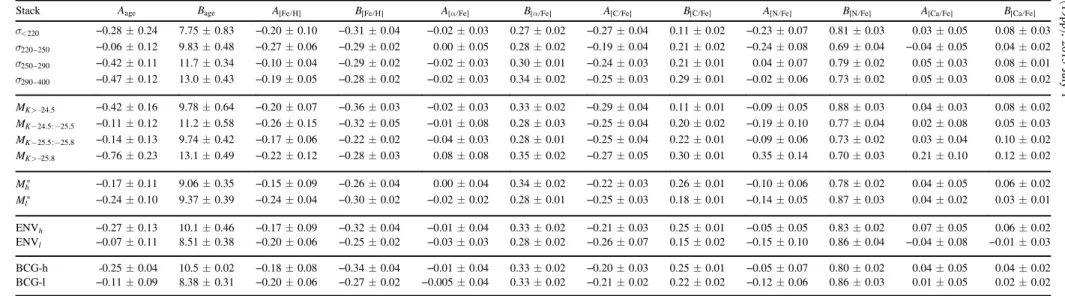
Stack A_age B_age A_{[Fe H]} B_{[Fe H]} A_[_a_Fe] B_[_a_Fe] A_{[C Fe]} B_{[C Fe]} A_{[N Fe]} B_{[N Fe]} A_{[Ca Fe]} B_{[Ca Fe]}

220 s< −0.28 ± 0.24 7.75 ± 0.83 −0.20 ± 0.10 −0.31 ± 0.04 −0.02 ± 0.03 0.27 ± 0.02 −0.27 ± 0.04 0.11 ± 0.02 −0.23 ± 0.07 0.81 ± 0.03 0.03 ± 0.05 0.08 ± 0.03 220–250 s −0.06 ± 0.12 9.83 ± 0.48 −0.27 ± 0.06 −0.29 ± 0.02 0.00 ± 0.05 0.28 ± 0.02 −0.19 ± 0.04 0.21 ± 0.02 −0.24 ± 0.08 0.69 ± 0.04 −0.04 ± 0.05 0.04 ± 0.02 250–290 s −0.42 ± 0.11 11.7 ± 0.34 −0.10 ± 0.04 −0.29 ± 0.02 −0.02 ± 0.03 0.30 ± 0.01 −0.24 ± 0.03 0.21 ± 0.01 0.04 ± 0.07 0.79 ± 0.02 0.05 ± 0.03 0.08 ± 0.01 290–400 s −0.47 ± 0.12 13.0 ± 0.43 −0.19 ± 0.05 −0.28 ± 0.02 −0.02 ± 0.03 0.34 ± 0.02 −0.25 ± 0.03 0.29 ± 0.01 −0.02 ± 0.06 0.73 ± 0.02 0.05 ± 0.03 0.08 ± 0.02 MK>-24.5 −0.42 ± 0.16 9.78 ± 0.64 −0.20 ± 0.07 −0.36 ± 0.03 −0.02 ± 0.03 0.33 ± 0.02 −0.29 ± 0.04 0.11 ± 0.01 −0.09 ± 0.05 0.88 ± 0.03 0.04 ± 0.03 0.08 ± 0.02 MK-24.5: 25.5- −0.11 ± 0.12 11.2 ± 0.58 −0.26 ± 0.15 −0.32 ± 0.05 −0.01 ± 0.08 0.28 ± 0.03 −0.25 ± 0.04 0.20 ± 0.02 −0.19 ± 0.10 0.77 ± 0.04 0.02 ± 0.08 0.05 ± 0.03 MK-25.5: 25.8- −0.14 ± 0.13 9.74 ± 0.42 −0.17 ± 0.06 −0.22 ± 0.02 −0.04 ± 0.03 0.28 ± 0.01 −0.25 ± 0.04 0.22 ± 0.01 −0.09 ± 0.06 0.73 ± 0.02 0.03 ± 0.04 0.10 ± 0.02 MK>-25.8 −0.76 ± 0.23 13.1 ± 0.49 −0.22 ± 0.12 −0.28 ± 0.03 0.08 ± 0.08 0.35 ± 0.02 −0.27 ± 0.05 0.30 ± 0.01 0.35 ± 0.14 0.70 ± 0.03 0.21 ± 0.10 0.12 ± 0.02 M_h* −0.17 ± 0.11 9.06 ± 0.35 −0.15 ± 0.09 −0.26 ± 0.04 0.00 ± 0.04 0.34 ± 0.02 −0.22 ± 0.03 0.26 ± 0.01 −0.10 ± 0.06 0.78 ± 0.02 0.04 ± 0.05 0.06 ± 0.02 M_l* −0.24 ± 0.10 9.37 ± 0.39 −0.24 ± 0.04 −0.30 ± 0.02 −0.02 ± 0.02 0.28 ± 0.01 −0.25 ± 0.03 0.18 ± 0.01 −0.14 ± 0.05 0.87 ± 0.03 0.04 ± 0.02 0.03 ± 0.01 ENVh −0.27 ± 0.13 10.1 ± 0.46 −0.17 ± 0.09 −0.32 ± 0.04 −0.01 ± 0.04 0.33 ± 0.02 −0.21 ± 0.03 0.25 ± 0.01 −0.05 ± 0.05 0.83 ± 0.02 0.07 ± 0.05 0.06 ± 0.02 ENVl −0.07 ± 0.11 8.51 ± 0.38 −0.20 ± 0.06 −0.25 ± 0.02 −0.03 ± 0.03 0.28 ± 0.02 −0.26 ± 0.07 0.15 ± 0.02 −0.15 ± 0.10 0.86 ± 0.04 −0.04 ± 0.08 −0.01 ± 0.03 BCG-h -0.25 ± 0.04 10.5 ± 0.02 −0.18 ± 0.08 −0.34 ± 0.04 −0.01 ± 0.04 0.33 ± 0.02 −0.20 ± 0.03 0.25 ± 0.01 −0.05 ± 0.07 0.80 ± 0.02 0.04 ± 0.05 0.04 ± 0.02 BCG-l −0.11 ± 0.09 8.38 ± 0.31 −0.20 ± 0.06 −0.27 ± 0.02 −0.005 ± 0.04 0.33 ± 0.02 −0.21 ± 0.02 0.22 ± 0.02 −0.12 ± 0.06 0.86 ± 0.03 0.01 ± 0.05 0.02 ± 0.02

Note.Fits to stellar population paramaters as a function of physical radius. For each parameter X, we ﬁt a relation X=A log (R R3–6kpc)+ . R3–6kpcB is the third radial bin, so B represents an effective value for the

stellar population property, while A is the radial gradient. These fits are done to stellar population properties derived from bins of (in order from top to bottom)s , M_* K, MKat fixeds , environment or halo mass at fixed_*

*

s , and then halo mass for only the brightest galaxy in the halo.

(11)

comparing radial trends as a function of mass ands (Spolaor_*

et al.2010). We therefore create four bins of K-band magnitude,

based on 2MASS photometry (Jarrett et al. 2003; Skrutskie

et al.2006): MK > -24.5(21 galaxies),-24.5>MK > -25.5

(23),-_25.5>MK > -_25.8(24), and MK < -25.8mag (19;

Figure6). We note that there is a wide range of stellar velocity

dispersion at each mass bin (Figure1), so this binning scheme is

truly different from the dispersion bins presented above.

Figure 5.Variation in stellar population parameters X as a function ofs (left) and M_* K(right). Left: we compare the relation measured from the coadded central ﬁbers

(open circles; dashed lines) with those from fits to the profiles weighted to1–1.5Re(filled circles; solid lines) and 3–6 kpc (crosses; long-dashed lines). We plot the fitted zeropoints (B) for each chemical property fitted vs. radius (Tables1and2_{) as a function of *}s . [Z/H] is estimated as [Z/H] = [Fe/H] + 0.94[α/Fe], which assumes that [O/Fe] tracks [Mg/Fe]. The power-law fits shown here have the form X₌A log ( */250 km s )_s -1 ₊B_{for each stellar population property X (Table}₃_{). We see}

that the central and 3–6 kpc ﬁts are generally similar and show the strongest trends withs , while when we scale to R_* ethe trends are washed out, supporting a scenario

where the inner 5 kpc collapsed quickly and scales with the galaxy potential, while the outer parts are accreted from lower-mass systems. Right: as above, but ﬁtting

X=A log (MK/ 25.3 mag)- +B.Note that the central measurement is missing for the highest MKbin because the Hβ measurement fell off the grid. In general the

dispersion in galaxy properties is larger in ﬁxed MKbins, and the trends weaker. The largest exception is [C/Fe] which shows a stronger correlation with MKthan *s .

10

(12)

Table 3

Galaxy Correlations at Varying Radii

Radius A_{[Fe H]} B_{[Fe H]} A_{[Z H]} B_{[Z H]} A_[_a_Fe] B_[_a_Fe] A_{[C Fe]} B_{[C Fe]} A_{[N Fe]} B_{[N Fe]} A_{[Ca Fe]} B_{[Ca Fe]}

σ* Fit Center _{−0.23 ± 0.43} _{−0.17 ± 0.03} 0.28 ± 0.47 0.12 ± 0.03 0.44 ± 0.15 0.31 ± 0.01 0.93 ± 0.22 0.37 ± 0.01 −1.25 ± 0.46 0.83 ± 0.03 −0.05 ± 0.22 0.06 ± 0.01 R 1–1.5 e −0.56 ± 0.28 −0.34 ± 0.02 0.02 ± 0.36 −0.06 ± 0.03 0.34 ± 0.18 0.32 ± 0.01 0.54 ± 0.11 0.16 ± 0.01 0.13 ± 0.26 0.77 ± 0.02 0.19 ± 0.25 0.09 ± 0.01 3–6 kpc 0.13 ± 0.20 −0.29 ± 0.01 0.63 ± 0.22 −0.02 ± 0.02 0.41 ± 0.12 0.30 ± 0.01 0.96 ± 0.11 0.19 ± 0.01 −0.33 ± 0.20 0.77 ± 0.01 0.15 ± 0.18 0.07 ± 0.01 MKFit Center _{−0.04 ± 0.04} _{−0.15 ± 0.04} _{−0.03 ± 0.05} 0.15 ± 0.05 0.01 ± 0.02 0.32 ± 0.02 -0.07 ± 0.03 0.38 ± 0.02 0.10 ± 0.04 0.80 ± 0.04 −0.02 ± 0.01 0.07 ± 0.02 R 1–1.5 e 0.02 ± 0.03 −0.36 ± 0.02 0.01 ± 0.03 −0.05 ± 0.03 −0.02 ± 0.01 0.34 ± 0.01 -0.03 ± 0.01 0.17 ± 0.01 0.03 ± 0.02 0.79 ± 0.02 −0.04 ± 0.02 0.09 ± 0.01 3–6 kpc −0.07 ± 0.02 −0.27 ± 0.01 −0.06 ± 0.02 0.01 ± 0.02 0.01 ± 0.01 0.31 ± 0.01 -0.09 ± 0.01 0.22 ± 0.01 0.09 ± 0.02 0.76 ± 0.01 −0.02 ± 0.01 0.10 ± 0.01

Note. Fits to stellar population paramaters as a function of σ* or MK, weighted to different radii. For each stellar population parameter X, we ﬁt a relation X=A log ( * 250 km s )s -1 +B (top) and

X=A log (MK/-25.3 mag)+B(bottom). X comes from the central binned data, from the fit in Table1weighted to1–1.5Re, and finally from the fits in Table2, weighted to 3–6 kpc.

(13)

As above, we ﬁt each stellar population property as a

function of radius, tabulated in Tables1 and2. Each effective

stellar population parameter is shown as a function of MK in

Figure5(right). Starting as in Section5.1by focusing on the

central measurements, we see that in general, there is more dispersion in stellar population properties (particularly

metalli-city and [Mg/Fe]) in a given MKbin as compared with a given

*

s bin. In particular, the second MKbin (−24.5 to −25.5 mag) shows considerably larger variance than the other bins. We believe that this larger error bar reﬂects a genuine increase in

the spread in stellar populations in this bin. At yet lower MK,

we no longer have a representative sample of objects. We also

generally see weaker trends in the stellar populations with MK

than withs , particularly in physically scaled bins (Table_* 3).

The exception is [C/Fe], which shows a more signiﬁcant

correlation with MK (12σ). We see no correlation with age or

[α/Fe]. There is, however, a marginal correlation with [Fe/H] (3σ) and a corresponding weak correlation with [Z/H]

(also 3σ). If we instead consider measurements from_1.5R_e, we

ﬁnd no signiﬁcant trends between stellar population properties

and MK(not even stellar age).

5.2.1. Bins in M*at Fixed σ*

We now ask whether, at ﬁxeds , there are residual trends in_*

the stellar population gradients as a function of stellar mass

(Figure 7). We create two luminosity bins divided at

MK = - mag (which approximately divides the sample in₂₅

Figure 6.Radial gradients in age, [Fe/H], [Mg/Fe], [C/Fe], [N/Fe], and [Ca/Fe] as above, but now in bins of MK(mag; a proxy for stellar mass) rather than stellar

velocity dispersion. Open symbols indicate cases where the primary measurement fell off the stellar population grid and we have used the median of the distribution of boot-strap stacks instead. The inversion program failed to converge for the [N/Fe] and [Ca/Fe] measurements for the outermost high-M RK e-scaled point, so no

measurement is shown. As indicated in the key, the bins have MK> -24.5(squares),-24.5>MK> -25.5(pentagons),-25.5>MK> -25.8(triangles), and

MK< -25.8mag (circles) respectively. We fit the radial gradients with a power law of the form X=A log(R R3)+Bfor each stellar population parameter X, where R3is either 3–6 kpc or1–1.5Re. Fits to the most massive (long-dashed lines) and least massive (dotted lines) galaxies are shown here; all fitted coefficients are

in Tables1and2.

12

(14)

two). We then enforce a matched distribution in s between_*

200 and 330 km s−1by creating 100 stacks for each mass bin,

each having an identical distribution ofs and each including a_*

total of 30 galaxies.

We find small but detectable differences in the two mass bins. Specifically, while the average stellar population ages are both ∼9.5 Gyr, we find that the high-mass bin is more α-enhanced by ∼0.1 dex with (possibly) correspondingly lower

[Fe/H] at ﬁxed Re (Table 1). The C and N abundances and

radial proﬁles are consistent with each other, but there is a hint that the more massive galaxies are also more Ca-enhanced at

ﬁxed *s . All of these trends could be qualitatively explained if

the timescale for star formation were shorter in the more massive systems, such that [Fe/H] is lower while [α/Fe] is higher and [Ca/H] follows [Fe/H].

The other possible explanation is that at ﬁxed s , more_*

massive galaxies are physically larger. This would explain why

at a ﬁxed fraction of Re, the more massive galaxies have lower

[Fe/H]. Graves et al. (2009) ﬁnd that galaxies with the lowest

central surface brightness also have the oldest ages and lowest [Fe/H] values, a similar trend to that seen here, albeit only for galaxy centers. When we have robust size measurements for our sample galaxies we will revisit the question of stellar populations through the Fundamental Plane, also including radial stellar population information.

5.3. Interpreting Stellar Populations Using Radial Trends There are a number of interesting trends seen in the stellar populations of elliptical galaxy centers that challenge our understanding, particularly when compared with Galactic

Figure 7.Radial gradients in age, [Fe/H], [Mg/Fe], [C/Fe], [N/Fe], and [Ca/Fe] as above, but now ins -matched bins of M_* K(mag; a proxy for stellar mass). Filled

symbols have MK< -25mag while open symbols have MK> -25mag. We ﬁt the radial gradients with a power law of the form X=A log(R R3)+Bfor each stellar population parameter X, where R3is either 3–6 kpc or1–1.5Re. The ﬁts to the high-mass (long-dashed lines) and low-mass (dotted lines) bins are shown here

and in Tables1and2.

13

(15)

trends. It is our hope that adding radial information will shed new light not only on the assembly history of ellipticals, but also on the nucleosynthetic yields that lead to these observed trends.

There are a few important caveats to keep in mind as we interpret the observations. First, our stellar ages, particularly at the center, are subject to large (∼2–3 Gyr) uncertainties. Thus, we caution against over-interpreting the radial trends in age at present. Some work covering larger dynamic range in radius do

detect clear age gradients (e.g., La Barbera et al.2012), but we

do not go to large enough radius to detect the very low metallicity true halo component that has been seen in a few

nearby cases (e.g., Harris et al. 2007; Williams et al. 2015).

Second, we remain cautious about the nitrogen measurements given the possible ﬂux calibration difﬁculties at the blue end of the spectrum. Third, recall that we are examining average trends in stacked spectra. Undoubtably there are interesting exceptions to all of these trends, and we plan to study the full range of parameters in future work.

We revisit our expectations for stellar population trends as a function of radius in light of the recent picture that galaxies form in two “phases,” an initial burst of in situ star formation creating the central component, followed by late-time accretion

of smaller, ﬂufﬁer units at larger radius (e.g., Naab et al.2009).

For galaxies in our mass range, the typical sizes of the central components are measured to be 2–5 kpc at z ≈ 2 (e.g., van der

Wel et al.2014). When we look at the stellar populations at this

typical radius (Figure5), we ﬁnd that age and [α/Fe] depend on

*

s rather than MK. Since we expect galaxies that form early to

be denser and have highers , a stronger correlation between_*

age and star formation timescale with s seems natural. In_*

contrast, [Fe/H], [C/Fe], and [N/Fe] depend more on the total stellar mass of the system.

In addition to considering a ﬁxed physical radius, we look at

stellar population trends at~_1.5R_e _(Figure 5_{). According to}

simulations, more massive galaxies are increasingly dominated

by accreted stars at radii beyond ∼5 kpc (e.g., Oser et al.2010).

Therefore we might expect the correlation between s and_*

stellar population properties to decrease when taken over the bulk of the stellar population. This is what we observe. Beyond

R_e

~ we ﬁnd no strong trend between s or M_* K and

abundances or abundance ratios. This result builds on what

we saw in Greene et al. (2013). There, we emphasized that the

stellar populations beyond Rein massive galaxies tend to have

low [Fe/H] ∼ −0.5 dex and high [α/Fe] ∼ 0.3 dex, stellar populations that are not seen in the centers of any galaxies

today (see also Bender et al. 2015). Here we see that beyond

Re, galaxies over a relatively wide range in s and M_* K have

similar abundances and abundance ratios, as expected if the more massive galaxies were built by accreting the less massive.

Only stellar age is still seen to increase at higher s when_*

examined at~R_e; we await better age measurements to verify

this result.

Another ongoing discussion in the literature regards carbon.

As is seen here, [C/Fe] is observed to increase with s in_*

elliptical galaxy centers (e.g., Trager et al. 1998; Graves

et al.2007; Johansson et al.2012; Conroy et al.2014). This is

in contrast to the behavior of carbon in the Milky Way or Local

Group dwarf galaxies (e.g., Kirby et al. 2015). To get such

super-solar carbon levels in the short timescales implied by the high ratio of [α/Fe], carbon must come not only from intermediate-mass (AGB) stars but also from massive stars

(Graves et al. 2007; Tang et al. 2014). Carbon yields from

massive stars are thought to increase with increasing metallicity

due to increased mass-loss from winds (e.g., Maeder 1992).

These same high yields at high metallicity are also invoked to explain abundance trends in Milky Way stars (e.g., Henry

et al. 2000). If true, we would expect that as the metallicity

decreases outwards in these elliptical galaxies, the [C/Fe] would

also decrease. This is what we observe (Greene et al. 2013).

Interestingly, we ﬁnd that the [C/Fe] gradient follows the

decline in [Fe/H] in both thes and M_* Kbins.

There is also considerable debate in the literature about the origin and behavior of nitrogen in elliptical galaxy centers

(e.g., Kelson et al.2006; Johansson et al.2012). Our surprising

results are two-fold. First, [N/Fe] is remarkably super-solar. Even assuming solar [O/Fe] (at odds with the observed [Mg/Fe]) [N/Fe] is found to be three times the solar value. Second, since the N is produced by C through the CNO cycle, their different behavior with radius is non-intuitive (and may point to a changing O abundance as well). As discussed above, the flux calibration at the blue end of the spectrum, containing CN, is quite uncertain. We do find good agreement between CN as measured from the SDSS spectra and the central Mitchell fiber. We also confirm that the CN measurements do not depend on how we treat the continuum. Including or excluding the overall continuum level in the stacks changes the CN1 measurement by <0.005 mag, resulting in very small <0.02 dex in the [N/Fe] ratio. To really confirm these high N abundance ratios at large radius, we would like to perform full spectral modeling to mitigate the impacts of blending and the uncertainties introduced by oxygen. In the meantime, it is interesting to note other stellar systems that display very super-solar nitrogen abundance ratios. For instance, in globular clusters, the wide range in [N/Fe] strongly suggests pre-enrichment by a previous early epoch of star formation (e.g.,

Cohen et al.2005).

Finally, we come to Ca. While nominally an α-element, it has long been known, based on both Ca4227 in the blue and the calcium triplet (CaT) index in the red, that Ca is under-abundant with respect to the other α elements (e.g.,

Cohen 1979; Terlevich et al. 1990; Vazdekis et al. 1997;

Worthey1998; Peletier et al. 1999; Proctor & Sansom 2002;

Saglia et al.2002; Thomas et al.2003; Choi et al.2014). Like

[Fe/H], [Ca/Fe] shows no dependence on s . There are a_*

number of explanations in the literature for the CaT measure-ments, including changes in the initial mass function (e.g.,

Cenarro et al. 2004) or a minority metal-poor population

(Saglia et al.2002). However, to explain both the blue and red

index behavior, it is more natural to presume that Ca behaves like an Fe-peak element because it is predominantly produced

in SNe Ia (e.g., Worthey 1998; Worthey et al. 2011; Conroy

et al.2014). As expected in that case, we measure a ﬂat [Ca/Fe]

ratio with radius. The one intriguing difference is the possible increase in [Ca/Fe] at large radius, which is worth pursuing.

5.4. Bins of Group Richness

While there are well-documented differences in the mor-phological mix of galaxies as a function of local galaxy density

(Dressler1980), the observations of environmental differences

in stellar population properties are quite subtle (e.g., Thomas

et al. 2005; Zhu et al. 2010; Lackner & Gunn 2013). Early

studies found evidence for younger ages in “ﬁeld” galaxies

(e.g., Terlevich & Forbes 2002). A number of other studies

14

(16)

report no change in scaling relations between stellar population

parameters and s as a function of local environment (e.g.,_*

Kuntschner et al. 2002; Bernardi et al. 2006), but do ﬁnd a

larger fraction of “rejuvenated” galaxies with recent star formation in low-density environments (e.g., Annibali

et al. 2007; Thomas et al. 2010). Recently, the samples have

grown large enough to evaluate not just the average properties of ﬁeld and cluster galaxies, but to control for stellar and halo

mass (e.g., Pasquali et al. 2010). For instance, Pasquali et al.

ﬁnd that satellite galaxies at ﬁxed mass grow older and more metal-rich as their host halo mass increases.

There is precious little literature on radial gradients in stellar populations as a function of group richness, although a few photometric studies ﬁnd steeper metallicity gradients in

lower-density environments (Ko & Im2005; La Barbera et al.2005).

Given our large sample and wide range of measured group

richness (Ma et al. 2014), we are in a unique position to

examine radial stellar population trends with environment. To divide the sample by richness, we use the group catalog

of Crook et al. (2007). When we divide our galaxies based on

group richness alone, the distributions in s do not match._*

Instead, there are more highs galaxies in richer groups. Since_*

*

s is strongly correlated with stellar population properties, we

must match thes distributions across different halo mass bins._*

Therefore, we divide the sample in half based on the number of neighbors: “low” comprises galaxies with no more than three

companions of L*> while “high” comprises the rest. The raw

distribution ofs have median_* á ñ =s_* 240km s−1for the

low-density bin and á ñ =s_* 260km s−1for the high-density bin.

Since there are not sufﬁcient numbers to further subdivide the

galaxies into bins ofs , we create 100 stacks, drawing from the_*

objects withs between 200 and 330 km s_* −1. We force the

low-Figure 8.Radial gradients in age, [Fe/H], [Mg/Fe], [C/Fe], [N/Fe], and [Ca/Fe] as above, but now in bins of group richness, controlling for the distribution ofs . Low_*

density (open squares) have three or fewer neighbors with L>L*, while ﬁlled circles include everything else. We ﬁt the radial gradients with a power law of the form

X=A log(R R3)+Bfor each stellar population parameter X, where R3is either 3–6 kpc or1–1.5Re. The ﬁts to the rich (long-dashed lines) and poor (dotted lines)

bins are shown here and in Tables1and2.

15