Isogeometric Simulation and Shape Optimization with Applications to Electrical Machines

(1)

HAL Id: hal-02275658

https://hal.inria.fr/hal-02275658

Submitted on 1 Sep 2019

HAL is a multi-disciplinary open access

archive for the deposit and dissemination of

sci-entific research documents, whether they are

pub-lished or not. The documents may come from

teaching and research institutions in France or

abroad, or from public or private research centers.

L’archive ouverte pluridisciplinaire HAL, est

destinée au dépôt et à la diffusion de documents

scientifiques de niveau recherche, publiés ou non,

émanant des établissements d’enseignement et de

recherche français ou étrangers, des laboratoires

publics ou privés.

Isogeometric Simulation and Shape Optimization with

Applications to Electrical Machines

Peter Gangl, Ulrich Langer, Angelos Mantzaflaris, Rainer Schneckenleitner

To cite this version:

Peter Gangl, Ulrich Langer, Angelos Mantzaflaris, Rainer Schneckenleitner. Isogeometric Simulation

and Shape Optimization with Applications to Electrical Machines. 12th International Conference on

Scientific Computing in Electrical Engineering, Sep 2018, Taormina, Italy.

�10.1007/978-3-030-44101-2_4�. �hal-02275658�

(2)

Optimization with Applications to Electrical

Machines

Peter Gangl1, Ulrich Langer2,4, Angelos Mantzaflaris3, and Rainer Schneckenleitner4

Abstract Future e-mobility calls for efficient electrical machines. For different ar-eas of operation, these machines have to satisfy certain desired properties that of-ten depend on their design. Here we investigate the use of multipatch Isogeometric Analysis (IgA) for the simulation and shape optimization of the electrical machines. In order to get fast simulation and optimization results, we use non-overlapping domain decomposition (DD) methods to solve the large systems of algebraic equa-tions arising from the IgA discretization of underlying partial differential equaequa-tions. The DD is naturally related to the multipatch representation of the computational domain, and provides the framework for the parallelization of the DD solvers.

1 Introduction

Isogeometric Analysis (IgA) is a relatively new approach for discretizing partial differential equations (PDEs). IgA was introduced in [2]. It can be seen as an al-ternative to the more classical Finite Element Method (FEM). The idea in IgA is to use the same basis functions for both representing the geometry of the

computa-Peter Gangl

Institute of Applied Mathematics, TU Graz, Steyrergasse 30, 8010 Graz, Austria e-mail: gangl@math.tugraz.at

Ulrich Langer

Institute of Computational Mathematics, JKU Linz, Altenberger Straße 69, 4040 Linz, Austria e-mail: ulanger@numa.uni-linz.ac.at

Angelos Mantzaflaris

Institute of Applied Geometry, JKU Linz, Altenberger Straße 69, 4040 Linz, Austria e-mail: ange-los.mantzaflaris@jku.at

Rainer Schneckenleitner

RICAM, Austrian Academy of Sciences, Altenberger Straße 69, 4040 Linz, Austria e-mail: rainer.schneckenleitner@ricam.oeaw.ac.at

(3)

2 Peter Gangl, Ulrich Langer, Angelos Mantzaflaris, and Rainer Schneckenleitner

tional domain and solving the PDEs. This aspect makes IgA especially interesting for design optimization procedures. In practice, it is often the case that one per-forms design optimization and geometric modeling simultaneously. State-of-the-art computer aided design (CAD) software uses splines or Non-Uniform Rational B-splines (NURBS) for the modeling process whereas the design optimization requires an analysis suitable representation of the model. So far the design optimization is mainly done using FEM as discretization method. Hence, the B-spline or NURBS representation of the geometric model has to be converted into a suitable mesh for the Finite Element Analysis. This conversion is in general very computationally de-manding. The new IgA paradigm circumvents these problems. Therefore, IgA is very beneficial for the simulation and optimization when the representation of the computational domain comes from CAD software; see [1, 11] for applications to electrical machines.

Since practical optimization problems tend to be very large, the numerical solu-tion of the underlying PDEs becomes computasolu-tionally very expensive. Moreover, in PDE-constrained shape optimization processes, there are more than one PDE to solve. In particular, line search requires to solve the magnetostatic PDE constraint several times. In order to get fast optimization results, we use Dual-Primal Iso-gEometric Tearing and Interconnecting (IETI-DP) methods for the solution of the linear algebraic systems arising from the IgA discretization. The IETI-DP solvers are non-overlapping domain decomposition methods; see [6, 7]. IETI-DP methods are closely related to the FEM-based FETI-DP methods; see, e.g., [10] and the references therein. We show that IETI-DP methods are superior to sparse direct solvers with respect to computational time and memory requirement. Moreover, IETI-DP provides a natural framework for parallelization. Indeed, our numerical experiments on a distributed memory computer show an excellent scaling behavior of this method.

The remainder of the paper is organized as follows. In Section 2, we describe our model problem and the shape optimization method that is based on the shape derivative. Section 3 is devoted to the IETI-DP solver and its performance on parallel computers. Finally, in Section 4, we use IETI-DP within the interior point optimizer Ipopt [12] yielding an efficient shape optimization procedure.

2 Shape optimization via gradient descent

2.1 Problem description

We investigate the simulation and shape optimization of an interior permanent mag-net (IPM) electric motor by means of IgA. The IgA approach seems to be very at-tractive for such practical problems. The most beneficial aspect of IgA in the context of optimization is the fact that the same basis functions which are used to represent the geometry of the IPM electric motor are also exploited to solve the underlying

(4)

PDEs. In the optimization procedure, we want to optimize the shape of the mo-tor in order to maximize the runout performance, i.e. to maximize the smoothness of the rotation of the motor. An example of an IPM electric motor is given in Fig-ure 1 (left). One possible way to optimize the runout performance of an IPM electric motor is to minimize the squared L2_{-distance between the radial component of the} magnetic flux B in the air gap and a desired smooth reference function Bd. The resulting optimization problem is subject to the 2d magnetostatic PDE as constraint. Mathematically, the arising optimization problem can be expressed as follows:

min D J(u) := Z Γ |B(u) · nΓ− Bd|2ds = Z Γ |∇u · τΓ− Bd|2ds (1) s.t. u ∈ H₀1(Ω ) : Z Ω νD(x)∇u · ∇η dx = hF, ηi ∀η ∈ H01(Ω ), (2) where J denotes the objective function, Γ is the midline of the air gap, Ω denotes the whole computational domain, and D is the domain of interest also called de-sign domain. The variational problem (2) is nothing but the 2d linear magnetostatic problem with the piecewise constant magnetic reluctivity νD(x) = χΩf(D)(x)ν1+

χΩmag(x)νmag+ χΩair(D)(x)ν0. Here, Ωf, Ωmag and Ωair denote the ferromagnetic,

permanent magnet and air subdomains, respectively, and ν1, νmag and ν0 denote the corresponding reluctivity values. Note that the shape D enters the optimization problem via the function νDand influences the objective function via the solution u. The right hand side F ∈ H−1(Ω ) in (2) is defined by the linear functional

hF, ηi :=

Z

Ω

(J3η + νmagM⊥· ∇η) dx (3)

for all η ∈ H₀1(Ω ). Here, M⊥denotes the perpendicular of the magnetization M, which is indicated in Fig. 1 and vanishes outside the permanent magnets, and J3 is the third component of the impressed current density in the coils. Note that the solution u is the third component of the magnetic vector potential, i.e. B(u) = curl((0, 0, u)T). Moreover, nΓ = (n1, n2, 0)T and τΓ = (τ1, τ2)T denote the outward unit normal and unit tangential vectors along the air gap, respectively.

We are interested in the radial component of the magnetic flux density along the air gap due to the permanent magnetization. For that reason, we set J3= 0 and con-sider the coil regions as air. Figure 1 (right) shows a quarter of a cross section of a simplified IPM electric motor that is provided by CAD software. Hence, this ge-ometry representation is suitable for IgA simulation. The red-brown areas represent ferromagnetic material (Ωf), the blue areas consist of air (Ωair), the yellow areas are the permanent magnets (Ωmag). The air gap of the motor is highlighted in light blue. In this initial model for the optimization, the design domain D is the ferromagnetic area right above the permanent magnets. In order to get a smoother rotation we are looking for a better shape of this part D.

(5)

Fig. 1 Real world IPM electric motor (see Acknowledgement) on the left, and a quarter of the cross section of a similar electric motor with 8 magnetic poles that is used in our numerical tests on the right.

2.2 The shape derivative

For the optimization of the IPM electric motor, we use gradient based optimization techniques. Hence, we need the derivative of the objective J with respect to a change of the current shape. The shape derivative in tensor form [4,8,11] of our optimization problem is given by dJ(D)(φ ) = Z Ω S (D,u, p) : ∂φdx, ∀φ ∈ H1 0(Ω , IR2) (4) withS (D,u, p) = (νD(x)∇u · ∇p − νmag∇ p · M⊥)I + νmag∇ p ⊗ M⊥− νD(x)∇p ⊗ ∇u − νD(x)∇u ⊗ ∇p, whereI denotes the identity, the state u solves the constraint (2), and p solves the adjoint problem

Z Ω νD(x)∇p · ∇η dx = −2 Z Γ (B(u) · nΓ− Bd)(B(η) · nΓ) ds ∀η ∈ H 1 0(Ω ). (5) In (4), S (D,u, p) : ∂φ means Frobenius’ scalar product of the 2 × 2 matrices S (D,u, p) and ∂φ = (∂ φi

∂ xj)

2

i, j=1, defined by A : B := ∑ni=1∑nj=1ai jbi j for general n× n matrices A = (ai j)ni, j=1 and B = (bi j)ni, j=1, whereas a ⊗ b := (aibj)ni, j=1 for vectors a = (ai)ni=1and b = (bj)nj=1from IRn.

(6)

2.3 Numerical shape optimization

We used a continuous Galerkin (cG) IgA discretization for both the simulation and optimization problems. The implementation is done in G+Smo1_{. Figure 2 (left)} shows a possible computational domain suitable for cG. The shown multipatch do-main consists of 93 patches. For each of these patches, we used a B-spline mapping from a reference patch with splines of degree 3. For the optimization, we need the shape gradient ∇J ∈ V := H₀1(Ω , IR2) which can be computed by solving the auxil-iary problem: find ∇J ∈ V such that

b(∇J, ψ) = −dJ(D)(ψ) ∀ψ ∈ V. (6)

The expression on the right hand side of (6) is the negative shape derivative whereas the expression b(·, ·) on the left hand side is some V -elliptic, V -bounded bilinear form which must be chosen appropriately. For our studies, we used

b(φ , ψ) = Z Ω φ · ψ dx + Z Ω α (∂ φ : ∂ ψ ) dx (7)

with a patchwise constant function α ∈ L∞_{(Ω ).}

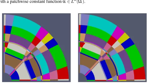
Fig. 2 Initial and final design of an IPM motor.

In the right picture of Fig. 2, we can see the optimized shape with respect to the runout performance compared to the initial domain on the left. We were able to reduce the objective from 4.236 · 10−4down to 2.781 · 10−4.

1 _{Mantzaflaris,} _A. _et _al.: _G+Smo _(geometry _plus _simulation _modules) _v0.8.1.,

(7)

3 Fast numerical solutions by IETI-DP

Up to now, we have solved the arising PDEs by means of a sparse direct solver. One drawback of a direct solution method is that it is rather slow for large-scale sys-tems. In particular, in shape optimization, we have to solve the state equation (2), the adjoint equation (5), and the auxiliary problem (6) for the shape gradient, which decouples into two scalar problems, in every iteration of the optimization algorithm. Moreover, during a line search procedure, it might be the case that the state equa-tion has to be solved several times. To overcome the issue of a slow performance, we were looking for a fast and suitable solver for our simulation and optimization processes. We chose the IETI-DP technique for solving the PDEs [6]. IETI-DP is a non-overlapping domain decomposition technique which introduces local subspaces which are then again coupled using additional constraints. A comparison between the sparse direct solver SuperLU [3] and IETI-DP for solving the state equation (2) on a full cross section of an IPM electric motor clearly shows that the recently developed IETI-DP method [6] performs much better as can be seen in Table 1. The numerical results displayed in Table 1 and Table 2 were obtained on RADON1 (https://www.ricam.oeaw.ac.at/hpc/overview/) a high performance computing clus-ter with 1168 computing cores and 10.7 TB of memory. Table 1 also shows that, with an increasing number of degrees of freedom, the proposed IETI-DP technique solves the problem much faster than the sparse direct solver. Moreover, it can be seen that, with too many degrees of freedom, the sparse direct solver ran out of memory whereas IETI-DP could provide the solution to the problem. The solution to the state equation is shown in Fig. 3 (right).

Table 1 SuperLU vs. IETI-DP on a single core.

# dofs SuperLU IETI-DP speedup 72 572 36.0 sec 17.0 sec 2.12 250 844 193.0 sec 69.8 sec 2.77 928 796 1943.0 sec 463.0 sec 4.20 3 570 332 – 1179.0 sec –

Moreover, IETI-DP provides a natural framework for parallelization. Because of the multipatch structure of the computational domains in IgA, each patch can be seen as a subdomain in the IETI-DP approach. Then one can create suitable subdomains consisting of a certain number of patches for each processor, e.g., one possible choice is to group the patches to subdomains according to their number of degrees of freedom which means that the degrees of freedom are almost evenly distributed over the number of processors. Table 2 shows the strong scaling behavior of the IETI-DP solver. In this experiment, we solved the constraint equation (2) on the full cross section of an IPM electric motor with 3 570 332 degrees of freedom.

(8)

Fig. 3 Whole initial cross section as well as the solution.

From Table 2, we can see the expected performance, i.e., if we double the number of processors the computation time reduces nearly by a factor of two.

Table 2 Strong scaling with IETI-DP and 3 570 332 dofs.

# cores 1 2 4 8 16 32 64 128 time [sec] 1179 577 325 164 89 43 22 14

rate – 2.04 1.78 1.98 1.84 2.07 1.95 1.57

4 Shape optimization based on Ipopt and IETI-DP

In this section, we point out the usage of the interior point optimizer Ipopt [12], for the shape optimization using IETI-DP as underlying PDE solver. If we perform shape optimization without any additional considerations, then we might run into troubles. More precisely, it can happen that we get self-intersections in the final shape even if the objective decreases.

To prevent such self-intersections, we consider the Jacobian determinant of the geometry transformation in the design domain and its neighboring air regions. The Jacobian determinant of these patches must have the same sign in each iteration. If the sign changes from one iteration to the next, then we reduce the step size until the Jacobian determinant of the new design has the same sign as in the initial configuration. In this way, we are able to ensure that the shape is technically feasible. In the first naive approach, all control coefficients of the multipatch domain are considered as design variables, and the vector field computed by (6) is applied

(9)

glob-8 Peter Gangl, Ulrich Langer, Angelos Mantzaflaris, and Rainer Schneckenleitner

ally. The computational effort for the optimization can be reduced by applying the computed vector field only on the important interfaces between the design domain and the neighboring air regions. This reduces the number of design variables from approximately 28000 to 128 in the coarsest setting. The inner control coefficients of the design area and the bordering air regions are rearranged via a spring patch model [9].

In a first test setting, Ipopt stops at an optimal solution after 95 iterations using a BFGS method. We set the NLP error tolerance to 10−6, the relative error in the objective change to the same value, and we decided to exit the optimization loop after three iterations within these error bounds. The objective value dropped from 4.266 · 10−4down to 2.587 · 10−4

Fig. 4 Optimal shape after 130 iterations with relaxed bounds (left), zoom into one of the design regions (right)

Furthermore, we tried an additional experiment were we relaxed the bounds on the constraints a bit. In particular, we set the bound relax factor in Ipopt to 1. The result of this experiment can be seen in Fig. 4. We may observe from Fig. 4 that we get a very smooth final shape with even a smaller objective value of 2.436 · 10−4. We point out that, if we adjust the different optimization parameters, we may get different optimal shapes and different objective values in the end.

Acknowledgements This work was supported by the Austrian Science Fund (FWF) via the grants NFN S117-03 and the DK W1214-04. We also acknowledge the permission to use the Photo in Fig. 1 (left) taken by the Linz Center of Mechatronics (LCM). The motor was produced by Hanning Elektro-Werke GmbH & Co KG.

(10)

References

1. Bontinck, Z., Corno, J., Sch¨ops, S., De Gersem, H.: Isogeometric analysis and harmonic stator–rotor coupling for simulating electric machines. Comput. Methods Appl. Mech. En-grg., 334, pp. 40-55, 2018

2. Cottrell, J.A., Hughes, T.J.R., Bazilevs, Y.: Isogeometric analysis: CAD, finite elements, NURBS, exact geometry and mesh refinement. Comput. Methods Appl. Mech. Engrg., 194, pp. 4135-4195, 2005

3. Demmel, J.W., Eisenstat, S. C., Gilbert, J.R., Li, X. S., Liu, J. W. H.: A supernodal approach to sparse partial pivoting. SIAM J. Matrix Analysis and Applications, 20(3), pp. 720-755, 1999 4. Gangl, P.: Sensitivity-Based Topology and Shape Optimization with Application to Electrical

Machines. Ph.D. thesis, Johannes Kepler University Linz, 2016.

5. Gangl, P., Langer, U., Laurain, A., Meftahi, H., Sturm, K.: Shape Optimization of an Electric Motor Subject to Nonlinear Magnetostatics. SIAM J. Sci. Comput., 37(6), pp. B1002–B1025, 2015

6. Hofer, C., Langer, U.: Dual-Primal Isogeometric Tearing and Interconnecting solvers for mul-tipatch dG-IgA equations. Comput. Methods Appl. Mech. Engrg., 316, pp. 2–21, 2017 7. Kleiss, S., Pechstein, C., J¨uttler B., Tomar S.L: IETI–isogeometric tearing and

interconnect-ing. Comput. Methods Appl. Mech. Engrg., 247, pp. 201–215, 2012

8. Laurain, A., Sturm, K.: Distributed shape derivative via averaged adjoint method and applica-tions. ESAIM:M2AN, 50 (4), pp. 1241–1267, 2016

9. Nguyen, D. M., Gravesen, J., Evgrafov, A.: Isogeometric analysis and shape optimization in electromagnetism. Ph.D. thesis, Technical University of Denmark, 2012.

10. Pechstein, C.: Finite and boundary element tearing and interconnecting solvers for multiscale problems. Springer, Berlin 2013

11. Schneckenleitner, R.: Isogeometrical Analysis based Shape Optimization. Master thesis, Jo-hannes Kepler University Linz, 2017.

12. W¨achter, A., Biegler, L.T.: On the implementation of an interior-point filter line search algo-rithm for large scale nonlinear programming. Math. Program., 106(1):25–57, 2006