Complex materials handling and assembly systems.

COMPLEX MATERIALS HANDLING AND ASSEMBLY SYSTEMS Final Report June 1, 1976 to July 31, 1978 Volume I EXECUTIVE SUMMARY by Stanley B. Gershwin John E. Ward Michael Athans

This research was carried out in the M. I. T. Electronic Systems Laboratory (now called the Laboratory for Information and Decision Ssytems) with support extended by National Science Foundation Grants NSF/RANN APR76-12036 and DAR78-17826.

Any opinions, findings, and conclusions or recommendations expressed in this publication are those of the authors, and do not necessarily reflect the views of the National Science Foundation.

Laboratory for Information and Decision Systems Massachusetts Institute of Technology

This report is a summary of research performed at the Massachusetts Institute of Technology Laboratory for Information and Decision Systems under National Science Foundation Grants APR76-12036 and DAR78-17826 since July, 1976. Details are reported in Volumes II - IX, and in 18 other papers, reports and theses referred to herein.

Topics discussed include analytic modeling of transfer lines and assembly systems having unreliable elements and finite buffers, equivalence between queueing models of transfer lines and assembly networks, compu-tational complexity, periodic scheduling, and in-process routing decisions.

It also contains the beginnings of the synthesis of the techniques deve-loped for these separate problems into an overall analytically-based methodology for design and analysis of flexible automated manufacturing

The research reported here has been carried out with the generous support of the National Science Foundation under Grants APR76-12036 and DAR78-17826. We have been fortunate to have the guidance of Dr. Bernard Chern, Program Manager, and Dr. Richard Schoen, Section Head (and Acting Program Manager). In addition to the authors, many faculty members,

research staff members, students, and visitors have contributed significantly to this effort. These personnel are listed in Section 6. We have also

been guided by a Steering Committee whose members are listed in Section 7.

Page

ABSTRACT i

ACKNOWLEDGEMENTS ii

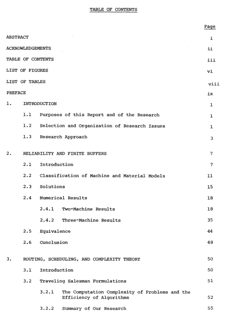
TABLE OF CONTENTS

LIST OF FIGURES vi.

LIST OF TABLES

PREFACE ix

1. INTRODUCTION 1

1.1 Purposes of this Report and of the Research 1 1.2 Selection and Organization of Research Issues 1

1.3 Research Approach 3

2. RELIABILITY AND FINITE BUFFERS 7

2.1 Introduction 7

2.2 Classification of Machine and Material Models 11

2.3 Solutions 15 2.4 Numerical Results 18 2.4.1 Two-Machine Results 18 2.4.2 Three-Machine Results 35 2.5 Equivalence 44 2.6 Conclusion 48

3. ROUTING, SCHEDULING, AND COMPLEXITY THEORY 50

3.1 Introduction 50

3.2 Traveling Salesman Formulations 51

3.2.1 The Computation Complexity of Problems and the

Efficiency of Algorithms 52

3.2.2 Summary of Our Research 55

3.3 Periodic Scheduling 64

3.3.1 Introduction 64

3.3.2 Principal Definitions and Results 68

3.4 Flow Optimization 74

3.5 Summary 86

4. SYNTHESES 90

5. PLANT VISITS 94

5.1 Kingsbury Machine Tool Corporation, Keene, NH 95 5.2 Raytheon (Headquarters, Lexington, MA) 100 5.3 Raytheon - Marine Products, Manchester, NH 101 5.4 Raytheon Missile Systems (Andover, MA) 101

5.5 Raytheon Data Systems (Norwood, MA) 102

5.6 Xerox Corporation (Rochester, NY) 103

5.7 Sundstrand Machine Tool Corporation, Belvedere, IL 106 5.8 General Motors Technical Center, Warren, MI 107 5.9 Electronic Associates, Inc., West Long Branch, NJ 108

5.10 AMP, Inc., Harrisburg, PA 109

5.11 GTE Laboratories, Waltham, MA 111

5.12 Scott Paper Company, Philadelphia, PA 112

5.13 AMF Harley-Davidson, York, PA 113

5.14 AVCO Corporation, Lycoming Division, Williamsport, PA 114 5.15 Sundstrand Aviation Division, Rockford, IL 114

5.16 Kearney and Trecker, Milwaukee, WI 115

5.17 Pratt and Whitney Aircraft, E. Hartford, CT 115 (also Middletown, CT)

5.18 Visits to MIT and Other Interactions 117

6. PERSONNEL 119

7. STEERING COMMITTEE 120

8. PROJECT DOCUMENTS 121

8.1 Reliability and Finite Buffers 121

8.1.1 Published Paper 121

8.1.2 Conference Proceedings 121

8.1.3 MIT ESL/LIDS Reports 121

8.2 Routing and Scheduling 122

8.2.1 Published Papers 122

8.2.2 Conference Proceedings 123

8.2.3 MIT ESL/LIDS Reports 123

8.3 Syntheses 123

8.4 Other Documents 124

8.4.1 Conference Proceedings 124

8.4.2 MIT ESL/LIDS Reports 124

8.4.3 Bachelor's Theses 125

9. OTHER REFERENCES 126

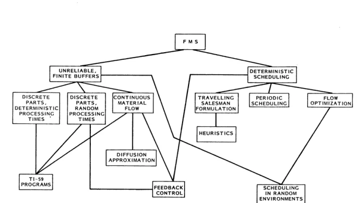
PAGE Figure 1.1 Organization of Flexible Manufacturing System Studies 4

Figure 2.1 Transfer Line. 8

Figure 2.2 Assembly Network. 8

Figure 2.3 Assembly - Disassembly Network. 9

Figure 2.4 Taxonomy of A/D Network Models. 12

Figure 2.5 Steady-state line efficiency for two-machine lines with the same first machine and different second machines

--Deterministic Processing Time Model. 20

Figure 2.6 Steady-state line efficiency plotted against the efficiency in isolation of the second machine, for two-machine lines with identical first machines. The curves are for N = 0, 4, 10, 20, 30, 40, 50, a. Deterministic Processing Time

Model. 21

Figure 2.7 The probability that the first machine in a two-machine line is blocked, plotted against storage capacity

--Deterministic Processing Time Model. 22

Figure 2.8 The probability that the second machine in a two-machine line is starved, plotted against storage capacity

--Deterministic Processing Time Model. 23

Figure 2.9 Expected in-process inventory plotted against storage capacity, for two-machine lines with identical first

machines -- Deterministic Processing Time Model. 25 Figure 2.10 Expected in-process inventory as a fraction of storage

capacity plotted against storage capacity, for two-machine lines with identical first two-machines --

Deter-ministic Processing Time Model. 26

Figure 2.11 Effect of Machine Speed on Production Rate and Average

In-Process Inventory -- Exponential Processing Time Model. 28 Figure 2.12 Effect of Machine Failure Rate on Production Rate and

Average In-Process Inventory -- Exponential Processing

Time Model. 29

Figure 2.13 Effect of Machine Repair Rate on Production Rate and Average In-Process Inventory -- Exponential Processing

Time Model. 30

Figure 2.14 Effect of Storage Size on Production Rate and Average

In-Process Inventory -- Exponential Processing Time Model. 31

PAGE Figure 2.15 Production Rate vs. Service Rate of the First Machine

--Erlang Processing Time Model. 33

Figure 2.16 Production Rate vs. Service Rate of the Second Machine

--Erlang Processing Time Model. 33

Figure 2.17 Production rate for discrete two-machine line. 34 Figure 2.18 Performance measures plotted against storage capacity N

--Continuous Material Flow Model. 34

Figure 2.19 Average in-process inventory plotted against storage

capacity N -- Continuous Model. 36

Figure 2.20 Performance measures plotted against processing speed of

stage 1, p1 -- Continuous Model. 36

Figure 2.21 Steady-state line efficiency for a three-machine transfer

line with a very efficient third machine. 38 Figure 2.22 Steady-state line efficiency for a three-machine transfer

line with a very efficient first machine. 39 Figure 2.23 Steady-state line efficiency for a three-machine transfer

line with identical machines. 40

Figure 2.24 Variations in the failure probability of one machine

affecting line efficiency. 41

Figure 2.25 Variations in the failure probability of one machine

affecting expected in-process inventory. 43

Figure 2.26 Parts and holes. 46

Figure 2.27 A Two-Buffer, Three-Machine Equivalence Class. 49 Figure 3.1 A Simple Example of a Two-Machine Flowshop Problem. 59

Figure 3.2 Optimal Schedule for Zero Buffer. 60

Figure 3.3 Optimal Schedule for Unity Buffer. 60

Figure 3.4 A Four-Machine Flexible Flowshop. 65

Figure 3.5 An Example of FFS Scheduling Problem. 72

Figure 3.6 A Two-Workstation System. 78

PAGE Figure 3.7 Optimal Split X as a Function of ~1 81

Figure 3.8 Optimal Average Queue Lengths as a Function of ~1 with

Q = 10. 83

Figure 3.9 Optimal Production Rates as Functions of pi₁ 84

Figure 3.10 Queue Occupation for Four-Machine Six-Piece System. 88

Figure 4.1 Small Decision Network 91

Figure 4.2 Preliminary Results from the Discrete Decision Network. 92

LIST OF TABLES

Table 2.1 Part-Hole Duality 47

Table 3.1 Monte Carlo Simulation Results 63

Table 3.2 tk. Matrices and Operational Requirements for ij,

Six Part Example 85

Table 3.3 Optimal Strategy Assignments 87

This report is a summary of research performed at the Massachusetts Institute of Technology Laboratory for Information and Decision Systems under National Science Foundation Grants APR76-12036 and DAR78-17826. The great volume of disparate material generated in the course of these projects has resulted in a rather lengthy summary. We have therefore further summarized it as follows.

Our goal has been the complete understanding of the systems aspects of flexible manufacturing systems (FMS's). The most important features of such systems are the unreliability of processors, the finiteness of buffers, and the need for routing and scheduling. To understand systems of such complexity, we first studied two kinds of simpler models.

First we studied transfer lines, i.e. production systems which have unreliable processors and finite buffers. This study was later expanded to include assembly (and disassembly). Routing and scheduling decisions do not appear here. Various model formulations have been treated and two-and three-stage systems have been analyzed numerically. Results are

pre-sented below, in Chapter 2.

The purpose of these models has been to represent.the filling and emptying of storages as a result of the failures and repairs of processors and the variations of processing times. These models will be useful to designers and purchasers of such equipment to answer such quesitons as: which of the machines under consideration should be used for a given processing stage? (that is, which offers the best trade off between cost, reliability, and production rate?) and where should buffers be located and how large should they be?

The concept of equivalence has been discovered. Systems of quite different layout -- such as a three-machine transfer line and an assembly network consisting of two processing machines, one assembly machine, and two buffers -- can have essentially identical behavior. In particular, their production rates are equal and their average levels of in-process inventory are related in a simple way.

Second, we have studied models of systems in which routing and scheduling decisions are required but in which stochastic effects

like machine failures are not important. Two kinds of formulations were investigated: one where discrete parts are represented individually, and one where material flow is represented continuously. In the former, issues of

reduce the computation. In the latter, the routing problem is formulated as a nonlinear programming problem.

We have only just begun to study the synthesis of these two problem areas. Exact solutions have been obtained for systems with a single routing decision, with two finite buffers, and with three machines which may or may not be unreliable.

1.1 Purposes of this Report and of the Research

The purpose of this report is to summarize the research work done at the MIT Laboratory for Information and Decision Systems (formerly the Electronics Systems Laboratory) in the area of manufacturing and

materi-als handling systems between June 1, 1976 and October 15, 1980 under National Science Foundation Grants APR76-12036 and DAR78-17826.

The research has been aimed at improving the low productivity in the manufacturing sector of the U.S. economy, which has been declining over the last several years. This decline has received a great deal of attention recently. Because of the need to improve productivity and be-cause of recent advances in computer hardware, we concluded early in this period that the manufacturing area presented an opportunity for research and applications of modern control and systems theory.

Our goal has been to understand generic issues, of interest to a wide range of industries, rather than to solve specific problems of immediate benefit.

We have surveyed the literature and visited many manufacturing facilities. As a result, we have chosen to direct our efforts along

certain lines and we have developed a corresponding research approach. In Sec-tion 1.2, we describe how our efforts are organized and in SecSec-tion 1.3

we demonstrate the approach that we have been following in each research area. Sections 2, 3, 4, and 5 briefly describe our technical work and plant visits. In Sections 6 and 7 we list the MIT personnel involved

in the project and the members of the Steering Committee. Our reports, published papers, conference proceedings and other documents are listed

in Section 8. Details on all areas of research can be found in these documents.

1.2 Selection and Organization of Research Issues

The main interests and capabilities of the MIT Laboratory for In-formation and Decision Systems are in the areas of optimization, control, dynamic systems, network analysis, mathematical modeling, and operations

research. We have concluded that these areas are relevant to certain crucial problems in manufacturing:

(1) The relatively little time workpieces (in batch production systems) are actually processed, compared with the great time they are in storage or being transported.

(2) The need to find the best use of modern computer and automated materials handling equipment in manufacturing facilities, particularly

flexible manufacturing systems.

There are, of course, many other pressing problems, such as the design of material processing equipment. However, our talents and

re-sources suggest that we concentrate on systems problem areas.

This decision requires that we treat manufacturing systems as com-posed of discrete components which have certain properties. Other than

studying these properties - such as processing time distributions, reliability behavior, and storage capacities - we do not treat the com-ponents in detail.

Our goal has been the complete understanding of systems aspects of flexible manufacturing system (FMS's). This includes the optimal opera-tion (including routing and scheduling) as well as the optimal design

(i.e., component selection to best perform a given manufactuing task) of an FMS. An FMS is a discrete part manufacturing system which is capable of automatically performing operations on a set of different parts with minimum changeover time. It has the following characteris-tics:

1. The production process can be represented by an automated network of flow of parts or material to be processed;

2. A variety of alternative production paths can be followed through the network, depending upon the work order to be processed or upon the availability of production units or work stations to process the work order;

3. The work orders to be processed are variable in size, nature, and economic value (batch manufacturing);

multiplicity of functions under the control of a central computer

or a local microprocessor or minicomputer;

5.

Interspersed among the production units are automatic inspection

or quality measuring stations.

We have not yet realized this goal.

However, we have made progress

in isolating important areas and studying them in great depth.

Consider Fig. 1.1, which represents the organization of our studies.

The features of an FMS that we felt are most important are:

(1) The unreliability of processing machines. Machines fail or require

maintenance at random or scheduled times, and they become unavailable

for a length of time which may be random or known in advance.

(2) The finiteness of buffer storage space. Buffers fill up orbecome

empty, and this may cause adjacent machines to be idle.

(3) The need for routing and scheduling. The full capability of an FMS

can only be realized if machines are not allowed to be idle.

Since a

computer controls the transportation system, and thus the routing and

scheduling of parts, it should be possible to minimize idleness.

As we point out in Section 1.3, our approach has been to isolate

the simplest nontrivial manifestation of these features, to isolate it,

to analyze it, and to then extend the analysis.

Consequently, we have

divided our research into areas where:

(1) there are unreliable machines and finite buffers, but no routing

or scheduling decisions; and

(2) routing and scheduling decisions must be made, but machines are

reliable and (in most cases) buffers are infinite.

The further subdivision of these areas is discussed in later

sec-tions. It should be noted that some of our current and future work is

aimed at reuniting the issues of reliability, finite buffers, and

on-line operational decisions.

1.3 Research Approach

Our choice of research approach has been heavily influenced by our

commitments to results of general rather than specific interest, and to

long range rather than immediate payoff.

It has led us to isolate

FMS

UNRELIABLE, DETERMINISTIC

FINITE BUFFERS SCHEDULING

DISCRETE DISCRETE ONTINUOUS TRAVELLING PERIODIC FLOW

PARTS, PARTS, MATERIAL SALESMAN SCHEDULING OPTIMIZAT

DETERMINISTIC RANDOM FLOW FORMULATION

PROCESSING PROCESSING TIMES TIMES HEURISTICSf //DIFFUSION APPROXIMATION\ TI-59 PROGRAMS E -FEEDBACK SCHEDULING CONTROL IN RANDOM ENVIRONMENTS

issues of general importance from their particular settings, and to

study them in ways that are intended to shed light on important areas,

although not necessarily solve problems with immediate economic effect.

For example, in studying unreliable systems with finite buffers, we have

concentrated on several abstract models of a transfer line.

In one

model, machines fail in a particular way, and buffers have limited

capa-city. However, it lacks many features that appear in real transfer lines,

to say nothing of FMS's.

For example, machines are assumed to have the

same deterministic processing time.

Different production stages may not

process workpieces in different cycle times. Failures are random, so

that a scheduled maintenance is not considered. They are geometrically

distributed and they affect machines separately.

Power failures, for

example, that affect the whole system are not considered. An unlimited,

ever-present supply of raw material is assumed, and there is constant

demand for finished goods.

All these features are important, but they would complicate an

al-ready difficult analysis. The choice of model to study is a matter of

judgment, and we believe that the model we have chosen has the most

qualitatively and quantitatively important features. Later study, by

our group or others, can extend the model to improve its realism, but

we believe that such a refinement must build on work like ours.

After an abstract model has been selected, it is analyzed

mathe-matically. Because such models are often intractable, it may be

modi-fied so that solutions can be obtained.

Part of what makes this work

dif-ficult is the need to choose a representation which is both faithful to

reali-ty (at least in some important respects) and can be studied with

mathe-matical tools that exist or that are developed for the purpose.

The next step is to construct a simulation and compare results.

This step is a substitute for testing our results in a factory setting

which would be expensive. A simulation is intermediate between

mathe-matics and reality because it can include many features of real systems

which cannot be included in analytic models. Simulation can also be

used to suggest the structure of the solution to a problem.

Finally, extensions are proposed and the cycle is repeated. The extensions may be intended to make the model more realistic (such as generalizing the exponential processing time transfer line model by

con-sidering Erlang processing times) or more general (such as concon-sidering assembly machines along with our transfer line models).

2.

RELIABILITY AND FINITE BUFFERS

2.1 Introduction

An important attribute of the components of manufacturing systems

is their reliability. Because of imperfections in design, normal wear,

and random effects that would be prohibitively expensive to eliminate

in advance, there are periods of time when components are not available.

A component may be undergoing routine maintenance, or it may be under

repair for failure.

For various reasons (e.g., the difficulty of

diag-nosing a failure), the length of time that a component cannot perform

its intended task can be modeled as a random variable.

Storages are present in many kinds of systems. They have the

ef-fect of decoupling the system so that changes from normal operating

con-ditions at one part of the system have minimal effect on the operation

of other parts of the system. While this is often useful, the precise

effect of such storages on system-wide behavior is only partially

under-stood.

We have made progress in formulating, solving, and understanding

a special class of system with storage - the flow shop or transfer line.

This class is illustrated in Figure 2.1. Workpieces enter the first

machine and are processed. They are then stored in the first storage

and proceed to the second machine and so forth. They leave the system

after the k'th machine.

Systems of this form are used in the manufacture of automobile

parts (Koenigsberg, 1959). They are used in the finishing of paper

products (Gordon-Clark, 1977), and in chemical processes, where the

"workpieces" are chemical batches and the machines are reactors (Stover,

1956).

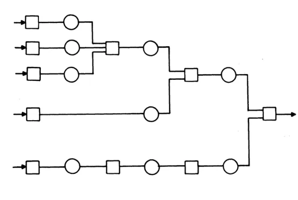
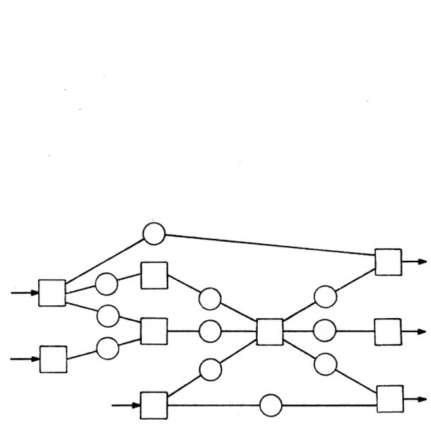
We have also considerably extended this analysis to treat networks

involving machines that perform assembly or disassembly operations. A

network performing assembly and unitary operations (where the latter are

operations on single parts, such as those in Fig. 2.1) appears in Figure

2.2, while a network in which assembly, unitary, and disassembly

opera-tions exist appears in Fig. 2.3.

(This network includes a machine that

does both assembly and disassembly.)

tMochn

oroe

chine

orog

Mochine

Figure 2.1 Transfer Line. Squares represent machines and circles represent buffer storages.

Figure

/

Disassembly Network2.3 Assembly

An important feature that all these networks share, and that allows the generalization of the analysis from transfer lines to assembly/dis-assembly (A/D) networks, is the fact that there are no choices to be made. The same kind of part, or set of parts, is always.presented to each machine, and the machine always does the same thing to it. Only one kind of part ever appears in each buffer.

One way in which buffers decouple systems is to isolate the effects of machine failures. When a machine downstream of a buffer fails, the buffer can provide space for partially manufactured pieces produced up-stream, and thus allow upstream machines to continue operating. In the absence of such buffering, the upstream machines would have to stop, reducing overall productivity. Even when storages are present, a pro-tracted failure can cause one or more storages to fill up. Similarly, a buffer can provide workpieces for the downstream part of the line when an upstream machine fails. Buffers also decouple systems in which the processing times are random. In such systems, a long processing time can act as a failure and, in the same way, cause other machines to be idle.

It is clear that storages that can hold more in-process inventory have a greater decoupling effect and thus provide a greater effective production rate (efficiency). However, increasing the sizes of such buffers leads to increased costs in the amount of space devoted to

stor-age and in the inventory itself. In order to choose the best trade-off

between these costs and the improvement in efficiency, it is necessary

that efficiency be calculated as a function of storage size.

Formulas for efficiency in the absence of buffers and in the

pre-sence of buffers of unlimited capacity are well known (Buzacott, 1967).

Also, efficiency can be calculated easily in systems with two machines

and a single storage of any size (Artamonov, 1977; Buzacott, 1967a;

Buzacott, 1967b; Okamura and Yamashina, 1977; Rao, 1975; Rao, 1977;

Sevast'yanov, 1962).

The behavior of longer systems has been formulated

in many ways (Sheskin, 1976; Hildebrand, 1968) and studied by

approxima-tion (Buzacott, 1967b; Buzacott 1972; Masso and Smith, 1974) and

simula-tic technique has been successfully obtained as yet. For a more com-plete survey of the analytic literature, see Schick and Gershwin (1978)* Gershwin and Schick (1980a, 1980b)*and Gershwin and Berman (1980)*

Our studies of these systems have two purposes. First, we feel that they can be of immediate economic importance in helping to design systems. High production rates are desirable, but they can only be achieved by increasing processing speed, reliability, or storage sizes, which may be expensive. These measures may also increase the amount of in-process inventory. Our studies can help to evaluate these trade-offs, Second, they can be of long range importance because they appear to be the first to use probabilistic models and obtain exact solutions to

systems with more than one finite buffer, and the first to study assembly and disassembly with queueing techniques. We anticipate that our work will lead to the analysis of more general systems, such as those with routing or scheduling choices.

2.2 Classification of Machine and Material Models

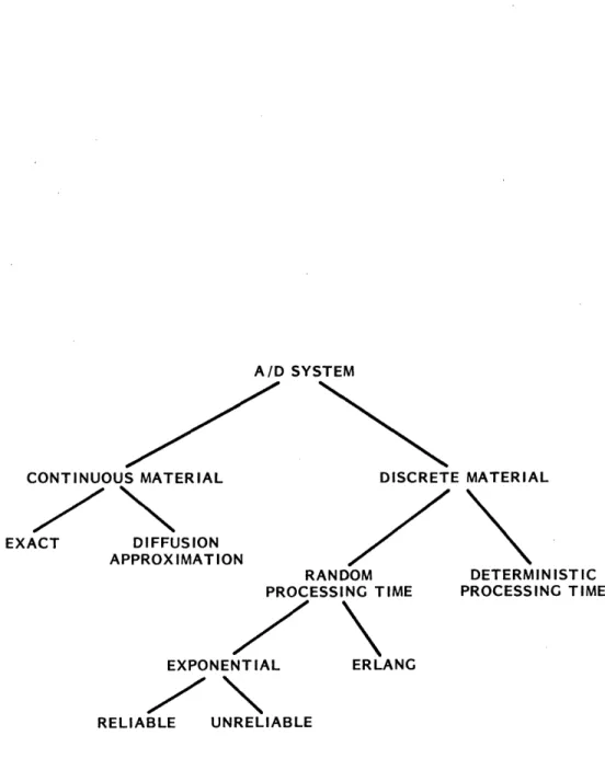
Figure 2.4 shows how the models of A/D systems we have studied are related. In all our studies, we have created Markov process represen-tations of these systems, in which the state is given by

s(t) = (nl(t),...,nkat),l , ( t )

a

k,M (2.1)

B M

where kB is the number of buffers, kM is the number of machines, ni(t)

is a variable representing the amount of material in buffer i, and aj(t) is a binary variable representing the repair state of machine j. The storage level variables satisfy

0 < ni(t) < Ni, i = 1,...,k B (2.2)

where Ni is the capacity of buffer i. (We use xi(t) to represent buffer

level in continuous material systems.)

The machine state variable has the following meaning:

References marked with an asterisk are documents describing work performed at the MIT Laboratory for Information and Decision Systems under National Science Foundation Grants APR76-12036 and DAR78-17826.

A/D SYSTEM

CONTINUOUS MATERIAL DISCRETE MATERIAL

EXACT DIFFUSION

APPROX IMAT ION

RANDOM DETERMINISTIC

PROCESSING TIME PROCESSING TIME

EXPONENTIAL ERLANG

RELIABLE UNRELIABLE

(0

if

machine j is under repair

a. =

j=l,...,

k

(2.3)

1 otherwise.

(In one study, machines are reliable, so the a(t) variables do not

ap-pear in s(t).

See Ammar and Gershwin (1980a)*.)

We have sought steady state probability distributions, from which

measures of performance can be calculated. These measures include the

production rate and the average in-process inventory level in each

buf-fer.

Other quantities, such as the expected time until a given

quanti-ty is produced and its second moment, can be obtained by other means

from a Markov process formulation.

We have presented exact solutions for models that represent the

flow of continuous material in Schick and Gershwin (1978)* and Gershwin

and Schick (1980b) .

These systems have two machines and a single buffer.

The machines are unreliable with both failure times and repair times

described by exponential probability distributions.

(We refer to these

systems simply as "continuous systems.")

Some of our current effort is

devoted to extending this analysis to larger systems.

The continuous model is characterized by three parameters for each

machine and one for each buffer. The buffer parameter is its capacity Ni:

the amount of material buffer i can hold. The rate at which machine i

processes material is pi. The rate that machine i fails is Pi.

That is,

the probability of a failure during a time interval of length 6t, which

is short, is pi6t.

Note that the mean time between failures (MTBF) is

then 1/p

i.

The rate of machine i repairs is ri.

This kind of model is appropriate to water purification plants,

petroleum refineries, etc., where the material to be processed actually

is continuous, or where a very large number of discrete parts are being

produced. The relationship between continuous systems and one model of

a discrete system is analyzed in the reports cited.

Some of our research efforts are dovoted to analysis and numerical

solutions of three-machine continuous systems. Additional effort

is devoted to alternative continuous network models and to diffusion

representations, which are approximations to these models. Reports on

these areas are in preparation.

Our other efforts are devoted to the analysis of systems with

dis-crete material. That is, the material to be processed consists of

separate workpieces, each operated on individually. The major distinc-tion is between systems with deterministic processing time and random processing time.

The former model (abbreviated as "deterministic") is appropriate when the set of pieces being treated are all the same, and where auto-mated machines perform the operations. An example is in high volume mass production by transfer line. In the models we have considered (in

Schick and Gershwin, 1978; Gershwin and Schick, 1979a, 1979b, 1980a; Gersnwin and Ammar, 1979; Ammar, 1980)*, all machines take the same

length of time to perform an operation; failure and repair time dis-tributions are geometric.

The deterministic model is characterized by a set of two numbers for each machine and one for each buffer. The probability machine i fails during an operation is Pi; the probability machine i is repaired during the time to perform an operation is ri; and the capacity of buffer j is N..

Machines with random processing times are appropriate when either (i) there is a mix of parts to be produced, and it is appropriate to

represent the mixture as random; or

(ii) the processors, perhaps because human operators are present, do not take a fixed length of time.

Both causes may be present. We have studied systems with exponential processing time (in Gershwin and Berman, 1978 and 1980; Gershwin and Ammar, 1979; Ammar and Gershwin, 1980)* and with the more general Erlang distribution for processing time (-Gershwin and Berman, 1978; Berman,

1979)*. In all our work, failure and repair distributions are tial, although there is at present work in progress on reliable exponen-tial systems. We refer to these systems as exponential (reliable or unreliable if a distinction is necessary) or Erlang.

The exponential processing time model is characterized by three numbers for each machine, as well as a capacity value for each buffer. Machines are specified by pi' the rate at which pieces are completed while machine i is working, Pi, the rate at which machine i fails, and ri, the rate at which repairs to machine i take place.

2.3 Solutions

Our studies began with transfer lines (Fig. 2.1) because they have the simplest possible structure. We have obtained analytic solutions, and studied qualitatively, continuous, deterministic, exponential, and Erlang two-machine transfer lines and deterministic three-machine

trans-fer lines. In addition, as we show below, the latter applies equally well to deterministic three-machine assembly and disassembly networks. Our current work is aimed at refining our three-machine solution tech-nique; applying it to other three-machine models, and extending it to larger systems.

To find the steady-state probability distribution of a discrete state Markov process, it is necessary to solve a set of M linear transi-tion equatransi-tions in M unknowns, where M is the number of states of the

chain. In the A/D network problem, M is large, so an efficient method is required.

This problem does have a structure that can be exploited. Due to that structure, it is possible to find £ vectors gj (j=l,...,l), each of which satisfies at least M-Z of the transition equations. The number of equations which are unsatisfied for at least one vector is Q.

Con-sequently if the probability vector is expressed as a linear combination of these vectors

p

=

L

cj.j

(2.4)

j=l

then it is guaranteed to satisfy the M-Z equations each .j satisfies.

In order to satisfy the remaining equations, the coefficients c. must be appropriately chosen.

To do this requires solving I linear equations in I unknowns. Since 2 is much smaller than M, this is relatively easy to do. For example, in the two-machine deterministic transfer line, M = 4(N+l) where N is the capacity of the buffer and 1=2. In the two-machine exponential transfer line M is the same but 1=4.

In the deterministic three-machine line, M=8(N1+l)(N2+l) (where N.

is the capacity of buffer i) and k=4(N1+N2)-10. Clearly, when N₁ and N2 are large, I is much smaller than M. However, the 2 equations in the

I unknowns cl,... ,c are poorly behaved for large Z. It has been neces-sary to use extended precision (32 decimal place) arithmetic to obtain 5 decimal place precision in analyzing transfer lines with large

storages. Even though k increases more slowly than M, the number of system states, the value of Z still limits the size of the problem that can be treated. This increase prevents the method, as currently formulated, from being usefully applied to longer line. Effort is being devoted to overcoming these limitations.

This suggests a general technique for solving large scale structured Markov chain problems. It should be considered a philosophy however, rather than a mechanical tool. Applying this technique to specific problems necessitates a great deal of analytical work. The benefit of the method is that it uses the structure of the system to substantially reduce the size of the linear system to be solved. At the same time, there is a loss of sparsity and as a result, the problem may become ill-conditioned.

A method of this type applies to continuous systems. In that con-text, however, the C vectors are functions and thus infinite dimensional. The method has worked in the two-machine context; longer lines pose tech-nical difficulties.

In all systems, it has been necessary to classify states. This classification is presented in detail in Gershwin and Schick (1980ar. Internal states are those in which all storages are at intermediate levels; boundary states are all others. In deterministic systems, internal states satisfy

2 < ni < Ni_2, i=l,...,kB . (2.5)

In random processing time systems, internal states are those where

1<n n < N i ,..., kB (2.6)

In continuous systems,

o

< Xi < Ni, i=l,. ,kB (2.7)

characterizes internal states.

In all the systems we have studied, the M-Z equations satisfied by the C vectors are those associated with internal states. (In continuous systems, there are an infinite number of such equations and states.) The component of the 5 vector associated with each internal state in the discrete models (other than the Erlang model) can be written

k k

kB

n. m C.

T(s,u) = n

Xi

n Y y (2.8)

1 1

-i=l i=l

where s is given by (2.1) and

U

(X

%

1,

'.X

1

FY

...

ry

(2.9)

is a vector of parameters. In the continuous case,

kB kM a.

S(s,U) = exp

E

\.x.

i

Y.1

i1

1 1

i=

(2.10)

where

U

=

(X,...,k

Y

...

k

(2.11)

is the parameter vector.

The kB

+

kM parameters satisfy a set of kM+. equations called the

parametric equations. The first is of the form

kM

In

f(Yiri,Pi)

= 1

(2.12a)

i=l

or

kM E f(Yiri'Pi) =

0

(2.12b) i=l

The rest of the equations are of the form

i

x.

P

i = g(Yiri,Pi), i=l,....kM (2.13a)

jeU(i)

or

( ia ix C iar7; A i i g( i rip~i i=l,...,k (2.13b)

where D(i) is the set of buffers directly downstream of machine i. That is, D(i) is the set of buffers that receive material from machine i. The set of buffers that send material to machine i is U(i).

The significant point is that the structure of the equations is the same, even if the functions (f and g) or the equations chosen (a or

b) depend on the model. The solution of one model is thus the starting point for the solutions to others. Furthermore, as long as the U parameters

satisfy (2.12) - (,2.13), all internal equations are satisfied, regardless of the type of the system, the number of buffers, or the size of the buffers.

The boundary states can be classified. In the three-machine case, there are transient states (whose steady state probability is zero), edge states (in which one buffer is at a boundary value and the other is internal), and corner states (in which, neither buffer is internal). Larger systems have a correspondingly more involved boundary structure.

An extension to (.2.8) exists so that E(s,u) can be written for all states. While these functions can be stated compactly for edges, corner expressions tend to be complicated, at least in the deterministic case. It would be desirable to simplify these expressions because that would facilitate extensions to larger systems. Ammar (1980)* suggests some changes to the expressions of Gershwin and Schick (1979b and 1980a)* and proposes conjectures for larger systems.

2.4 Numerical Results

In this section, we present numerical results from the solutions of these models. It should be emphasized that the quantities calculated

(production rates, average in-process inventories, probabilities of starvation and blockage) are all determined from the steady state proba-bility distribution. Two-machine results are presented in Section 2.4.1; three-machine results appear in Section 2.4.2.

2.4.1 Two-Machine Results

Deterministic Processing Time Model

A set of examples from Schick and Gershwin (1978) illustrates the effects of increasing buffer sizes and making machines more efficient. Five sets of two-machine results were calculated: the first machines of all lines were the same; the buffer sizes varied over the same range

varied from a low value in case 1 to a high value in case 5. The

system bottleneck is machine 2 in cases 1 and 2, and machine 1 in

cases 4 and 5. Both machines are equally efficient in case 3. This

is well illustrated by the graphs of line efficiency and probability

of blocking and starving appearing in Figures 2.5 - 2.8.

The line efficiency is plotted against storage capacity for each of

the five cases in Figure 2.5.

In cases 3 - 5, the value of E(X) is the

same, since the least efficient machine is the first.

In cases 1 - 2,

on the other hand, the least efficient machine is the second one.

Thus,

E(X) changes as e

2

is varied. This effect is clearly seen in Figure 2.6,

where the line efficiency is plotted against the efficiency in isolation

of the second machine, e

2

, for various values of storage capacity.

The

production rate increases with e

2

until e

2

e

I

= .5, after which the

first machine acts as a bottleneck and the production rate approaches

an asymptote. Thus, beyond a certain point, increasing the efficiency

of the second machine becomes less and less effective.

This result

agrees with those for the flow through a network of queues conducted by

Kimemia and Gershwin (1980) .

In general, when a given attribute is

limiting, the flow through the network increases linearly with that

attribute; as the attribute increases, it is no longer limiting, some

other attribute is, and the flow rate reaches an asymptote.

It is noteworthy that for a certain range of e

2

, it appears that

providing small amounts of storage can improve the production rate as

much as increasing e

2

; for example, e

2

= 0.67 and no storage gives

approximately the same efficiency as e

2

= 0.6 and N=4, or e

2

= 0.5 and

N=10.

This is significant, because improving the efficiency of a machine

may involve a great deal of research and capital investment or labor

costs, and may thus be more expensive than providing a small amount of

buffer capacity.

It is especially important that this effect is strongest

when the machines have approximately the same efficiency, i.e., when

the line is balanced. Since this is most often the case in industry

(although deliberately unbalancing a line may at times be profitable

-see Rao, 11975; Hillier and Boling, 1966), the fact that increasing buffer

capacity is most effective when the line is balanced is of great importance.

Figures 2.7 and 2.8 are also revealing in that they show the

de-pendence of forced-down times on the efficiency of the second machine

and the storage capacity.

The probability that the first machine is

blocked (p(N,1,0)) is plotted against storage capacity in Figure 2.7.

U aU

8

g

8

E

'

=) C3, W IJ. IJ

C

CM~~~~~~~~~~~~~~~~~~4

-rl

ee..V) C~~~~~~~~~~~~~~~~~~~~~~~~~~~~~~~~~U

or E LO

O~~~~~~~~~~~~~~~~~~~~*O 0

'U)

.PU) O k~r U)0 0

~

· a)

r'))

_-rt 4-)1 U) -rd rl

-o

1

CUo

E.d

-CY 7, _{· 1 1~)}c) u r. If) 44l-I ,-4 It.4_0~ a Q) O If)

O

O a, .rl

,'{

In

u4:)

lcl~n 4

a)

0~~~F a) Aouspille ourl FX4~~~~~~~·l

0-)

0 1.0 a)

0-

to

~U) ~4

0

OD

dU) IC

~

~~

₀rO 4.1i 0 Q) HE-n

CM

ui IX

~~~~~~~~~~~~~~~~~~~~~~~~u

to

s~~~~~~~~~~~~~~~~~~~~~~~~~~~~_

,---Iu I~.\

_·

F 0~~~~~~ ₀

_~(d

(0

0

4-'

~~n

rr, a~~~ C ,.e 4-i C cJ _ _W

~~~~~~~~~0,

_{V) ·}

~~~~~~~~~~~~~~--I

.-wf

CO -iLO · r-7% a), H r .I-iH Q d

...

~~~~~~~~~~~~~~~~~~~~~~~~~~~~~~~~~~~~~~~~~~~~~~~~~~~1

H

-4-4 U 0 n ·U

No

~~~~~~~~

~~~~~r Q).~

_{H 8}

T

V4) " - a1) 0) Q) r~~~~~~d 44 tn '.-. C ,4J_a2) t~~~~~~~ -- C) 'v ") O U)

~.iE

_{a- oS or} %U_c a) 0

~~~O

0 I~~~ue!~~~~~!lla~~~ a

~

u c.' WH FT _{a)~l0 -H-}C 0

~~~4JO,--H4J

E

~~I.

a)

-H->.io

.

C.)n~ ,r-H

ia, h..

E

fit~~~~~~~~~~~~~~~~~~~~~~~~~~~~~~~~~~~~~~~~~9 U)w 00

o

cc~~~~~~~~~~~~~~~~~~~~~~~~~~~~~~~~~~~~I D1 *H()~ B

_{~~~~~~~~~~~~~~~~~~~~~~~~~~~~to}

r~~~~l U) * 0

o

_{o .1-i} '-I -~r ',-0- _{4J -H}* -n~~~n _{p, a)}0 )O_-0. a . iU .-0 a) 124 ..i

CD

r-

V .

(D

r

.cli

0

pepoojq si I

Ou.140DW

*D44

A411!qDqoJd

-)

I.I.) o

I~~~~~~EC

p,. C u

.0

E

c;

0~~~~~~

C)

Q).~

~

~ ~

~

~

~

~

~

~~~~~~.

u,~~~~~~~~~~~~~~~~~~~~u

O~~~~~~~

> UlU 0~~~~r _{0 -rl} 0 4U)_.~rl -rl 0 4-) -I rd;r 0 I U)~~~~~~~~~~~(, ' - ·r _{Q 0} ,

-P-O

co

44 .13 ·0

uO

rO

~..

Od

--o

~

p9AJ~~~~~~lS

~

S!u

UqDJ

P

'iE!~oO

-~-This probability approaches a positive asymptote when the second machine is least efficient, and hence the bottleneck. It approaches zero when the first machine is least efficient, so that as the storage capacity is allowed to increase without bound, the first machine is fully utilized because it is the system bottleneck. This result agrees with the findings of Secco-Suardo (1978)* and Kimemia and Gershwin (1980)*: as the speed

(and thus the production rate in isolation) of a machine increases, the average size of the queue decreases.

Conversely, the probability that the second machine is starved (p(.0,0,1)) is plotted against the storage capacity in Figure 2.8. It approaches a positive asymptote when the first machine is limiting. When the second machine is the system bottleneck, this probability approaches zero as storage increases.

The cost of providing storage may or may not increase linearly with capacity. However, the cost incurred by maintaining in-process inventory is not linear with buffer capacity because the expected process in-ventory does not increase linearly as capacity increases.

Okamura and Yamashina (1977) observe that for large enough buffer capacities, an increase in the capacity does not necessarily imply an increase in the expected number of pieces in the storage. This is illustrated by the results presented in Figures 2.9 and 2.10.

In Figure 2.9, the expected number of pieces in the storage is plotted against storage capacity. In cases 1 and 2, the first machine is more efficient than the second, and the expected in-process inventory increases with storage capacity. In case 3, the two machines have

equal efficiencies, and the expected inventory increases linearly with storage capacity. In cases 4 and 5, the second machine is more efficient than the first, and the expected inventory approaches an asymptote.

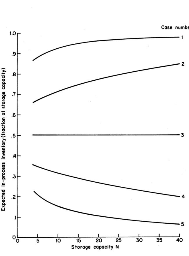
This is even more evident in Figure 2.10, where the expected in-process inventory as a fraction of the storage capacity is plotted against storage size. These curves approach limiting values.

Exponential Processing Time Model

Several cases were run by Gershwin and Berman (1980)* to illustrate the behavior of this model.

The graphs of the production rates (P(1) and P )) and average -(1) - (2))

4 E o'

o

*

\\

-\

I

I

I

~cr

44 &4

t 43 *H -H U) IC) 4-) -H Q0 4J 4J₀ 4-) -H tO Enrl

I I I~~~~~~~~~~~~~~~~~~~Q

II

I

c

Id

c i

zU

r

O34rl (n .4 4*H 43) 0

~43

244 U) 0 r. 4-H 0

0

IC)

0

IA

0

cl-i

'A)

CY

0

'A

0

4J~~~~~~~~~~~~~~~~~~~~c

AJOIUGAUI

ssa:)ojd-ui p,94:)dx3

C.,.' 0)

~~\\\\

I rlct~~-·

·

rz

Case number

1.0

.9-2

.8-0

.6

-o 0 o C 0

_ .5

0

._

C Q. .

0

I

I

I

I

I

0)

5

10

15

20

25

30

35

40

Storage

capacity N

Figure 2.10 Expected in-process inventory as a fraction of storage capacity plotted against storage capacity, for two-machine lines with identical first machines -- Deterministic Processing Time Model.

plotted in Figure 2.11. The superscripts refer to case numbers.

In case 1, as p1' the rate of service for machine 1, increases, the production rate P increases to a limit. That is, there is a saturation effect, and no amount of increase in the speed of machine 1 can improve the productivity of the system. Note that as the first machine is speeded up, the average amount of material in the storage, n, increases.

In case 2, in which p2 is varied, the production rate for P

increases. When the second machine is very fast, it frequently empties the storage. Consequently n decreases and machine 2 is often starved.

In cases 3 and 4 failure rates pi are varied. System production rates P() an and a average in-process inventories are plotted in Figure 2.12.

In both cases, as Pi increases, production rate decreases. As before, when the second machine is more productive, n is small, and when the first machine is more productive, n is large.

Figure 2.13 contains the graphs of production rates and average in-process inventories for cases 5 and 6, in which rl and r2 are varied.

Again, as a machine becomes more productive (ri increases), the system's production rate increases. As in the previous cases, when the first machine becomes more productive, n increases and when the second becomes more productive, n decreases.

-The model's behavior, in these six cases, have the following characteristics in common: as any machine becomes more productive,

due to pi or ri increasing or Pi decreasing, the system's production rate increases. The average in-process inventory increases when the first machine becomes more productive, and it decreases when the second machine becomes more productive.

In Figure 2.14 are plotted the production rate and average in-process inventory for case 7, in which the storage size, N, is varied from 2 to 20

As N increases, the production rate appears to increase to a limit. This limit seems to be the production rate in isolation of the least pro-ductive machine (Pl). (See Buzacott (1967b)). Note also that as N + X , n approaches a finite limit. This is evidently because machine 2 is the more productive stage in this system.

Ic

~~~~0

_{o o}

0

0

_o

0

0

's

ri

'~

I

II

~~~~~~~I0

I~~~~~~~~~~~~~

*1-II

~cU)

I

_I

_{~~~~~~~~~~~~~~I}

I

H U)

0~~

I~~~~~~~~~~~

I

I ₁ g)

C)

~II

0 O~~~

I

_I

_H~~~~~~~~~~~I

I

_~~~~~~~I

i

0)

0~~~~~~~~~~~~~~~~~~~~

_4U)

I

~~~J"

I

A('I

I

o

o

I

-I

/H-I=~~~~~~~~~~~~~~~~~~~~=

D.40,~

~

~

I~~~~~~~~

4J) 044 0 4-P

\

~

~

~~~~~~~I

' ~~

I

/~~~

_{/~~~~~a o}

c~~~~~l CP (Q c~~~~~~~~~~~~~~~~~l CN~~·l

~

H -I_E!

/~~~~~~~~

.O

I

q4u-I~~~~~~~~

c

~

o

~.

(q

~.

C\

. ou

E,

c

-

0

I

O

O'

_O.OI

r~i

Nl

0

o

4

I

~~~~~~~~I

I

o

=

_

~~ ~

ou

a)

I

_[-'4

I~~~~~~~~

I

H_oa 0

I

$4

o

p4

o

g

I~~~~~~~~~~~~~~~~~~~~~~I

/

_/~~~~

0I

a) tO

I~~~~~~~/

_/

4 \

_\~~~~~~~~L

cu J.)

₀

Pao

"

~~o

o

I

',

a~-

o

I

.,-t

ed

o

4J

I~~~~~~~~~~~~~~~~~~~~~~~~~~~~~~~~.-4.4 o)

o.. I

~~~~~~~~~~~~~~~~~~tc

I'

:

ic:

I-I

_HH OD a0 B~

~

~~

c OH

I!;

I J

I

4' -- :~~~~c

CL~~~~~~~~~~~~~~C

fj

I

Qa)Io 'H(

Q

0

II

'

I

01

H

IC)

~

~

~

I

U)P U)_U~ O~~~O

ui~I

o

0 I' I 0~~

LIl

_I

IH

_I

₀

-P

I

9

I

_I

I

0

~II

-II

_{I~~~~~~~~~~~~~~~~~~}

_I

I

_fi

_~~~~~~~~~~.I

'

II

U I

I

i 4-)

I~~~~~~~

/

I~~~~

Id

/

0a)0 A..

CI

4U) 44 U

l~~~~~~~~~~r

_{~~~~~~~~~~~~~~~'I}

\~~~~~~~~~~+ o~

/I

_It

_/

\

0

~

/

I

_rl

0

(co

N

0

( .1-I

____

(D

d

O

0

Cd 0 E0 4I 0 H U) E-e

z .

_{O H}-i IC 0 \Is_ CD 4

o~0

N u1

II--\Or

'-iO \ W0 A~~~~~~~~~C qUa

Ed-(|

IC Ii)

C

o

(D o

:

0

n

C

-The purpose of these numerical experiments is to demonstrate that the model behaves reasonably well. Because production rate and mean in-process inventory are easy to calculate, the model should be a useful tool for manufacturing engineers to use in evaluating alternative con-figurations of two-stage transfer lines.

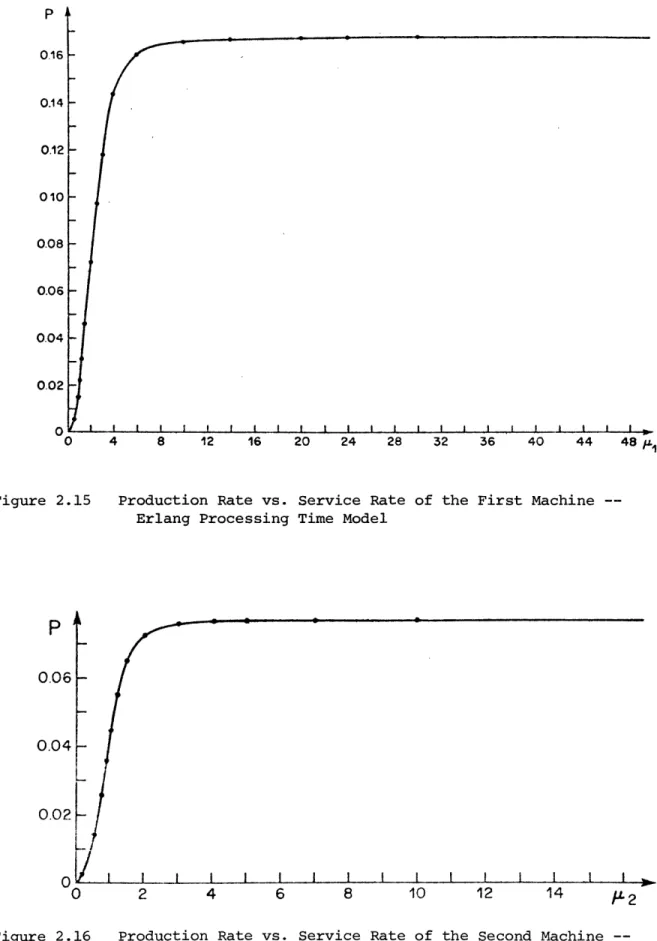
Erlang Processing Time Model

A set of numerical experiments were displayed by Berman (1979)*. This case is a generalization of the exponential processing time model.

Figures 2.15 and 2.16 show how the production rate and average in-process inventory vary with the speed of the first machine, This behavior

is similar to the other graphs, but it is interesting to see that these

curves are slightly s-shaped.

The 6-transformation

The 6-transformation was introduced in Schick and Gershwin (1978)*

and Gershwin and Schick (1980) for computing the production rate of some discrete systems with large storage capacities. The algorithm is based on the observation that the production rate is nearly preserved by the &-transformation; thus, the production rate of a deterministic processing time system with a large storage capacity may be approximated by that of a system with a small storage capacity, if the systems'

parameters are related in a certain way. The advantage of this approach stems from the fact that the computational effort required to compute the production rate. of a discrete system (as well as the memory require-ments, for production lines consisting of more than 2 stages) increases with its storage capacity.

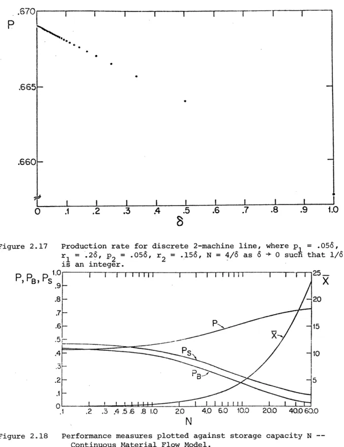
Figure 2.17 illustrates the behavior of the production rate of

a deterministic processing time system as 6 + 0 such that 1/6 is an integer. It is noteworthy that the limit of the discrete production rate as 6 + 0 is the production rate of the continuous system. Furthermore, the range of the· production rate over 0 < 6 < 1 varies by only about 1.7%, which would be a reasonable approximation for some applications.

Continuous Model

The production rates, forced down times (.expected fractions of time during which the first stage is blocked or the second is starved) and average in-process inventories of some continuous systems are plotted in

P 0.16 0.14 0.12 010 0.08 0.06 0.04 0.02 0 4 8 12 16 20 24 28 32 36 40 44 48 p.

Figure 2.15 Production Rate vs. Service Rate of the First Machine --Erlang Processing Time Model

P

0.06

0.04

0.02

0 2 4 6 8 10 12 14 2

Figure 2.16 Production Rate vs. Service Rate of the Second Machine --Erlang Processing Time Model

.670

PI

.665,

.660

0

.i

.2

.3

.4

.5

.6

.7

.8

.9

1.0

Figure 2.17

Production rate for discrete 2-machine line, where p

=

.056,

r 1= .26, 2 = .056,

r

2 = .156, N = 4/6 as 6 + 0 such that 1/6

is an integer.

PI PB1

PS

_

I

'

25-29

-

< <Ox

.8 -

-

20

.2 -

5

.1

.2 .3 .4.5.6 .8

1.0

20

4.0 6.0

10.0

20.0

40.0 60.0

N

Figure 2.18

Performance measures plotted against storage capacity N

--Continuous Material Flow Model.

Figures 2.18 - 2.20.

In Figure 2.18, the storage capacity N varies in the range [.1, 60]. The production rate is seen to approach asymptotes as N + 0 and N + 0. The first stage has the lowest production rate in

isolation. Thus, it becomes the bottleneck as N + a. It is shown in Schick and Gershwin (1978)* that the forced down probability of a bottle-neck stage in a discrete line approaches 0 as N + c. Accordingly, PB tends toward zero as the storage increases in Figure 2.18.

If the first stage in the line is less productive than the second, the average in-process inventory reaches a limit (Schick and Gershwin

(1978))*. This is not evident in Figure 2.18, where x appears to be increasing without bound. However, this is only because x does not level off for the storage capacity range [.1,60]. The average in-process

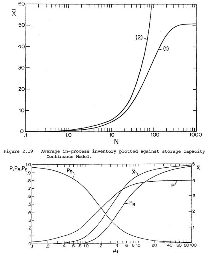
inventory for the same system parameters is plotted in Figure 2.19

(Curve 1) for the range [.1, 1000]. Here, it is clear that x approaches a limit as N + a. This also implies that the average fraction of the buffer

storage utilized approaches zero as N -+ 0. The average in-process inventory for a system where stages 1 and 2 have bee:n switched is also plotted on Figure 2.19 (Curve 2). Here, x increases without bound, since

the upstream stage is now more productive than the downstream stage. Furthermore, the average in-process inventories for the original and reversed production lines are complementary, i.e., add up to N (see

Schick and Gershwin (1978), Ammar (1980), and Ammar and Gershwin (1980)) . Finally, the performance measures are plotted against p1I the proces-sing speed of the first stage, in Figure 2.20. As p1 increases, the

average in-process inventory increases. This is natural since the upstream stage puts more material into the storage than the downstream stage

can remove, for large p.₁ As a result, pS decreases while PB increases. The production rate of the system, P, increases with p₁ for small p1

until the second stage becomes limiting, at which time P approaches

an asymptote. The asymptote is the production rate in isolation of stage 2. 2.4.2 Three-Machine Results

Three-machine results are available only for the deterministic

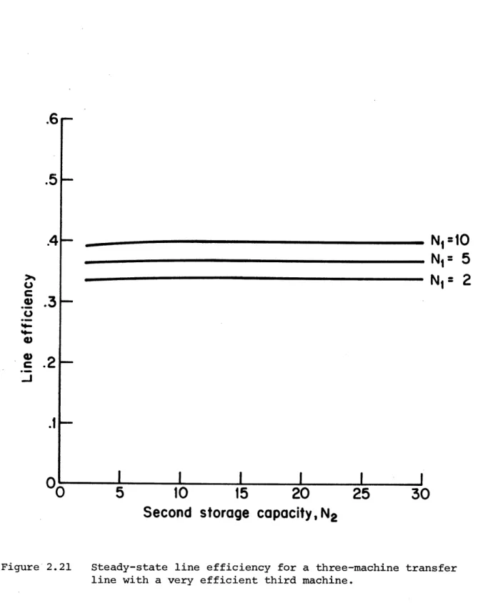
processing time model. Some results were calculated by Schick and Gershwin (1978)*. They appear in Figures 2.21 - 2.23 where the line efficiency is plotted against the capacity of one of the storages, while the other is held to two or three values.

50

(2).

40

-t)

30

20

10-0Ol

II

I I

11 I

I

I I I

lll

1

0.1

1.0

10

100

1000

N

Figure 2.19 Average in-process inventory plotted against storage capacity N --Continuous Model. 1.0 It I I I

5-.8

4-

.,

,_

3 .1 .1 .2 .4 .6 .8 1.0 2 4 6 8 10 20 40 60 80100

Figure 2.20 Performance measures plotted against the processing speed of stage 1, p1 -- Continuous Model.

In Figure 2.21, the last machine is most efficient, so that

workpieces produced by the second machine are most often instantly

processed by the third machine, Thus, the second storage is often

nearly.empty, and little is gained by providing it with a large

capa-city. On the other hand, the efficiency in isloation of the first

machine is close to that of the downstream segment of the line (i.e.,

the portion of the line downstream of it, consisting of machine 2,

storage 2, and machine 3).

Thus, it is not profitable to provide

storage space between machines 2 and 3, though it is useful to provide

a buffer between machines 1 and 2.

In Figure 2.22, the first machine is most efficient. Thus,

the first storage is often nearly full, and the downstream segment of

the line operates most of the time as if in isolation. On the other

hand, the efficiency of the third machine is close to that of the

upstream segment of the line (machines 1 and 2, storage 1).

Thus, little

is gained by providing the first storage with a large capacity, although

it is useful to have a large storage between machines 2 and 3.

In Figure 2.23, all machines have equal efficiencies in isolation,

and the effects of added storage capacity are most clearly visible in

this case. Furthermore, it is observed that the production rate is

symmetrical with respect to the orientation of the system. See Section 2.5.

These examples indicate once again that storages act best as

buffers to temporary fluctuations in the system. If the efficiencies

of machines are very different, storages do not improve production

rate; if the line is well balanced, the temporary breakdowns are to a

certain extent compensated for by buffer storages.

Pomerance (.1979)* performed a large number of numerical experiments

with three-machine lines. She made a similar observation about system

symmetry which influenced the development of the equivalence concept

summarized in Section 2.5.

Figure 2.24 shows how variations in the failure probability of

machine 3, p

₃

, affect line efficiency, E. The curves represent different

values of the failure probability of machine 2, P

₂

.

All other input

parameters are constant, as indicated. Note that the first machine has

a high efficiency in isolation (el = .8), and should not be a bottleneck.

.6

.5

.4

N,

-10

N1= 5

-

_

N

I

1 2

C

m

J3

.2

0

15

20

25

0

5

10

15

20

25

30

Second storage capacity,

N

2

Figure 2.21 Steady-state line efficiency for a three-machine transfer line with a very efficient third machine.