HAL Id: hal-02426400
https://hal.inria.fr/hal-02426400
Submitted on 2 Jan 2020
HAL is a multi-disciplinary open access
archive for the deposit and dissemination of
sci-entific research documents, whether they are
pub-lished or not. The documents may come from
teaching and research institutions in France or
abroad, or from public or private research centers.
L’archive ouverte pluridisciplinaire HAL, est
destinée au dépôt et à la diffusion de documents
scientifiques de niveau recherche, publiés ou non,
émanant des établissements d’enseignement et de
recherche français ou étrangers, des laboratoires
publics ou privés.
Improving cable length measurements for large CDPR
using the Vernier principle
Jean-Pierre Merlet
To cite this version:
Jean-Pierre Merlet. Improving cable length measurements for large CDPR using the Vernier principle.
CableCon 2019 - 4th International Conference on Cable-Driven Parallel Robots, Jun 2019, Cracow,
Poland. �hal-02426400�
using the Vernier principle
Jean-Pierre Merlet
J-P. Merlet, HEPHAISTOS project, Universit´e Cˆote d’Azur, Inria, France [email protected]
Abstract. Cable lengths is an important input for determining the state of a CDPR. Using drum with helical guide may be appropriate for small or medium-sized CDPR but are problematic for large one. Another issue is the initialization of the cable length as measurements based on drum rotation are incremental. We propose to address automatic initialization and improvement of cable length measurements by using regularly spaced color marks on the cable combined with color sensors in the mast of the CDPR. We show that this disposition allows one to automate the initialization issue and then how it allows to get regularly accurate estimation of the cable length by using the Vernier principle.
Keywords: cable length, accuracy, initialization, calibration
1
Introduction
Measuring the cable lengths of CDPR with rotary winch is usually done by measuring the rotation of the drum with an encoder. Coiling the cable on the drum is usually done in two manners: the drum may have a spiral guide and a guiding mechanism moves synchronously the cable in front of the free part of the spiral or the cable is just coiled on the fly on the drum. An alternate to using rotary actuators is the use of linear actuator with a pulley mechanism that amplifies the stroke of the actuator [Merlet(2008)] but we will not consider this case in this paper. The spiral-guided mechanism is the one used in many cases for small to medium sized CDPR such as IPANEMA [Pott et al(2012)] or COGIRO [Gouttefarde et al(2012)]. It leads to a one-to-one and fixed relationship between the cable length and the drum rotation and if elasticity can be neglected it provides an accurate measurement of the cable length but it has drawbacks:
– the drum may accept only a single layer. This limits the available total cable length as increasing the drum radius will both increases the length measurement inaccu-racy due to error in the drum rotation measurement and the necessary motor torque for a given cable tension. Hence such a mechanism may not be appropriate for very large CDPR that involves coiling several dizains or hundreds meters of cable – the friction of the cable on the spiral guide increases the cable wear and cable
elasticity is not taken into account
Another issue for such a winch system is that the drum encoder usually provides only a relative measurement. When starting the CDPR it is therefore necessary either to cal-ibrate the platform’s pose [Alexandre(2012)], [Alexandre et al(2013)], [Chen(2004)], [Baczynski(2010)], [Miermeister and Pott(2012)] or to measure the initial length of the cable, both tasks being tedious. To the best of the author knowledge an automatic deter-mination of the initial cable lengths has not yet been presented. We propose a method that allows both to obtain the initial cable lengths and provides regularly information on the cable length.
2
Approach
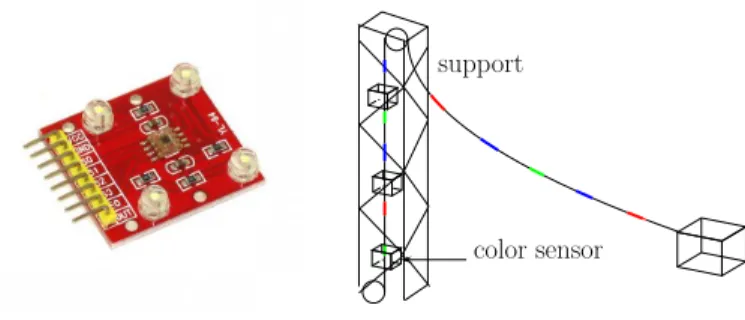
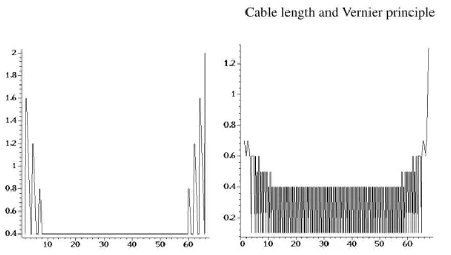
Our method is directly inspired by a method we have implemented successfully on our MARIONET-ASSIST CDPR [Merlet(2010)]. This CDPR uses synthetic cables and we have glued several aluminium foils on the cables at known distance from the platform cable attachment point B. At the winch level the cable goes through two electrically isolated Delrin guides that have been covered with aluminium foils, the mid-point be-tween the guides being the output point A of the winch. Each time a cable foil goes through the guides an electric contact is established providing a boolean information for the control computer. Using this event a semi-automated procedure may be used for initialization (the robot stops when detecting a foil and the operator input manually the corresponding cable length) and, in operation, for updating the current estimation of the cable length. In this paper we propose to improve this method by using colored marks on the cable and several color sensors in the mast that constitute the support structure of the CDPR (figure 1) for benefiting from a Vernier scale. Color sensor consists in leds that provides a constant illumination and receptors that are sensitive to a particular color (figure 1). Such sensors are inexpensive and our tests have shown that they can reliably detect at least the three RGB colors. They can easily be integrated in the support mast in small non transparent boxes with a circular opening for the cable (figure 1), the color sensor being protected from external illumination.
color sensor support
1
3
The initialization problem: a first approach
A major problem for CDPR is to determine automatically what are the cable lengths at the start of the operation. The basic idea of our approach for automatizing this ini-tialization process is the detection by a color sensor of n successive color marks when coiling (or uncoiling) the cable, while having disposed the colors marks on the cable in such a way that there is only a single occurrence of any n successive colors on the cable. For example if we use 3 possible colors R, G, B for the mark, then there will be, for example, a single GBR sequence on the whole cable, the other sequences being any triplet among the set (R, B, G), possibly with repetition (for example GGG or GGB). Let us assume that a given color sequence (n1, n2, n3) has been detected and that dlis the
known distance between A and the color sensor. As a given color sequence (n1, n2, n3)
is unique on the cable the detection of n3gives us the corresponding mark number on
the cable and consequently the distance d between B and the mark. The cable length ρ= ||AB|| is therefore obtained as ρ = d − dl. Hence there is a one-to-one relationship
between all possible sequences (n1, n2, n3) and ρ. Therefore the initialization method
consists simply in uncoiling the cable until we have at least n marks between a color sensor and the B point and then coiling the cable until the color sensor has detected n marks, such a process being easy to automatize. A faster initialization process will be presented in section 5.3.
4
Number of marks
As will be presented in the next sections we also intend to use the marks to update the current cable length. Intuitively it makes sense to have a large number of marks on the cable for that purpose, but our initialization process imposes the constraint of having a single occurrence of n successive marks, whatever is the color combination. We will now investigate the influence of this constraint on the maximal number of marks on a cable. Assume that we use marks with k different colors: our problem is to determine the maximal number of marks m that we may have on the cable so that all subsets of n successive marks are different in term of color value. In other words we have to determine the largest color sequence that satisfy this constraint. This prob-lem is well known in combinatorial theory and such a sequence is called a De Bruijn sequence [Bruijn(1975),Bruijn(1946)]. For a cable with k possible mark values that has all n combination of the mark values a single time in the sequence, the sequence length (i.e. the number of marks) is knfor a cyclic sequence. So for n= k = 3 we have a sequence of length 27. But as our sequence is not cyclic we may add 2 additional marks (but not 3, which will be contradictory) so we may have up to 29 marks on the cable. An example of such sequence (the colors are indicated by the number 1, 2, 3) is: [12312112213222323313111333212]. Using this coding the detection of 3 successive colors by a color sensor allows one to determine the location of the last mark on the cable and consequently the cable length.
For n= 4 the De Bruijn sequence has a length of 34= 81. and we may add 3
additional marks while keeping the property so that we will end up with a total of 84 marks on the cable. For k= 4 colors and a sequence of n = 3 marks the De Bruijn
sequence has a length of 64 to which we may add 2 marks for a total of 66 marks while for a sequence of n= 4 marks we will have a total of 259 marks on the cables. We have now to examine how the marks may be used to determine the cable length.
5
Measuring cable lengths
The height of the tower will be denoted h (in the examples we will assume h= 15) and we assume that there is a color sensor every dmmeters starting from the base of
the tower so that we have kmax sensors in the tower with kmax= f loor(h/dm), where
f looris the largest integer lower than h/dm. The cable sensor will be numbered from
1 to kmax, the sensor kmax being the highest in the tower. We have k1max marks on the
cable that are assumed to be distributed regularly on the cable, the distance between two successive marks being denoted by dcmeters.The marks are numbered from 1 to
k1max, mark k1
max being the one the closest to B. The distance between mark k1max and
the attachment point B, called the dead length, will be denoted by b. When the cable is completely uncoiled we assume that the first mark on the cable is located at the kmax
sensor. The total length Lt of the cable between the base of the tower and B is
Lt= kmaxdm+ (k1max− 1)dc+ b (1)
If we assume that the k1-th mark is located at the k-th color sensor, then the cable length
Lbetween the color sensor and B is: L= (k1
max− k1)dc+ b (2)
and the length ρ of the cable between A, B is then obtained from L by subtracting the distance h − kdmbetween the k-th sensor and the top of the tower:
ρ= (k1max− k1)dc+ b − (h − kdm) (3)
Consequently the lowest value ρminfor ρ is obtained for k1= k1max and k= 1 with the
value ρmin= b − h + dm
We will choose b= h−dmso that this minimum is 0 in order to have always positive
ρ when a mark lies in front of a color sensor. Consequently ρ is obtained as:
ρ= (kmax1 − k1)dc+ (k − 1)dm (4)
By taking all possible values for k, k1we get all ρ that will correspond to a mark
detection by a color sensor, that we will call a sensor event, and is defined by a triplet (k1, k, ρ) corresponding respectively to the mark number, to the sensor number and the
corresponding cable length.. As k, k1lie respectively in[1, kmax], [1, k1max] there will be
at most k1maxkmax different ρ. This is an upper bound as the same ρ may possibly be
obtained for different pairs(k1, k). For these values of ρ we will get a sensor event that
will allow us to determine the cable length between A, B.
Sorting by increasing value all possible values of ρ and taking the differences be-tween successive values will provide the various cable length changes ∆ ρ bebe-tween two sensor events. Note that ∆ ρ cannot exceed dm which correspond to the case where a
given mark is seen successively by the same color sensor. Between two sensor events the cable length will be interpolated from the measurement of the drum rotation with some uncertainty because of modeling error on the coiling process. Clearly there is an interest of having the largest possible number of significant sensor event (i.e. one that provides an update on the cable length), a relatively flat distribution of the ∆ ρ with a low average value. Another interest of a flat distribution is that we may relate two successive sensor events (which will provide a change ∆ ρ in the cable length) to the corresponding drum rotation ∆ θ in order to obtain an estimate of the mean drum radius that will be updated at each sensor event. This estimate will then be used to determine the cable length between two sensor events.
5.1 Significant sensor events
Clearly we are interested in having the largest number of different ρ. Consequently we should avoid having two sensor events for the same ρ. In other words we have to determine if we may have ∆ ρ equal to 0 being given dm, dc. Consider now 2 sensor
events defined by the triplets (k1, k, ρ), (k01, k0, ρ0). Using equation (4) we may calculate
the ∆ ρ= |ρ − ρ0| as
∆ ρ= |(k01− k1)dc+ (k − k0)dm|
There is a symmetry in this relation as, being given the events (k1, k), (k01, k0) we will get
the same ∆ ρ for the events (k01− k1
max, kmax− k0,), (k1max− k1, kmax− k0). Let us assume
that the ratio dm/dcis a rational number p/q and consider the rational number
p1 q1 = k1− k 0 1 (k − k0)
which is such that |p1| is the lowest possible value for |k1− k01| while |q1| is the minimal
value of |k − k0|. We have ∆ ρ= dc|(k − k0)( −p1 q1 +p q)| (5)
As dc is a known positive constant the minimum of ∆ ρ will be obtained when |(k −
k0)(−p1 q1 +
p
q)| is minimal. As |(k − k 0)| ≥ |q
1| the minimum of ∆ ρ is obtained for the
rational p1/q1that is the closest to p/q.
Equation (5) is essential to assert the distribution of the ∆ ρ. For example for k1max=
29 (29 marks on the cable) and dm= 2.4 (which leads to kmax = 6) and dc= 2 we
get dm/dc= 1.2 = 6/5. If we set p1= 6, q1= 5 we get k1− k01= 6 leading to k1=
k01+ 6 ∈ [7, 29] and k01∈ [1, 23]. We have also k − k0= 5 and as k cannot exceed 6 we get k0= 1, k = 6. The ρ obtained for the pair (k1∈ [7, 29], 6) will be the same than for
the pair (k1− 6, 1) so that we will get 23 identical ρ. As the maximum number of ρ is
29 × 6= 174 there will be 174-23=151 different ρ available. .
However we are not only interested in discarding the sensor events that will give the same ρ but also in the set of ∆ ρ that are lower than dm. Hence we have to find the
positive rationals p1/q1with a denominator at most equal to kmax− 1 and lower or equal
the following theorem that is used for studying the Farey sequences1:
Theorem 1: Let s= a/b and t = c/d > s and if there is no rational between s and t with a denominator that is lower than the largest b or d, then bc − ad= 1 and the rational with smallest denominator between s and t isb+da+c.
Let us illustrate the application of this theorem in our previous example for dm= 2.4
and dc= 2. We have t = p/q = 6/5 and we are looking for s that is smaller than t
so that there is no rational between s,t with a denominator that is smaller than a, 5. According to the theorem we must have 6b − 5a= 1 that is clearly satisfied for a = b= 1. Then according to the theorem the next rationals having the lowest denominator are 7/6, 13/11 and so on with increasing denominator. As the denominator are larger than 5, then the closest valid rational p1/q1to p/q, that is lower than p/q, is 1/1. As
b= k − k0we get the minimal ∆ ρ as dc× (−1 + 6/5) = dc/5= 0.4. For any ρ obtained
for the pair(k1, k), then the ρ obtained for the pair (k1+ 1, k + 1) will differ from the
previous one by 0.4.
We may now examine the closest valid rational p1/q1to p/q, that is larger than
p/q. Using the theorem we get the condition 5c − 6d= 1 that is fulfilled by c = 5, d = 4 leading also to ∆ ρ= 0.4. For being more systematic we may use the following theorem
Theorem 2: let two rationals a/b and c/d and let u= p/q the rational closest to c/d and larger than c/d with denominator lower or equal to n. Let k be the largest integer such that k ≤(n + b)/d. The value of p, q are given by
p= kc − a q = kd − b
We will use this theorem by starting from the lowest possible successive value for a/b, c/d which are 1/(kmax− 1), 1/(kmax− 2) and construct the full Farey sequence or
order 5 corresponding to .dm= 2.4 and dc= 2. We get the following pairs (p/q, |∆ ρ|):
(1/1 or 5/4, 0.4), (4/3, 0.8), (3/2, 1.2), (2/1, 1.6), (7/5, 2). Note that ∆ ρ= dmis always
possible by setting k1= 1, k = kmax, k= kmax− 1. But although we have obtained what
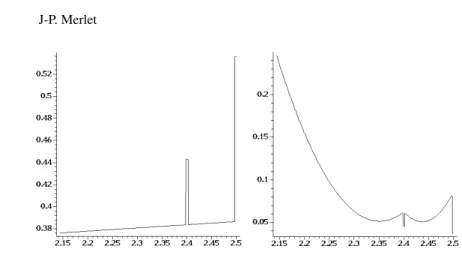
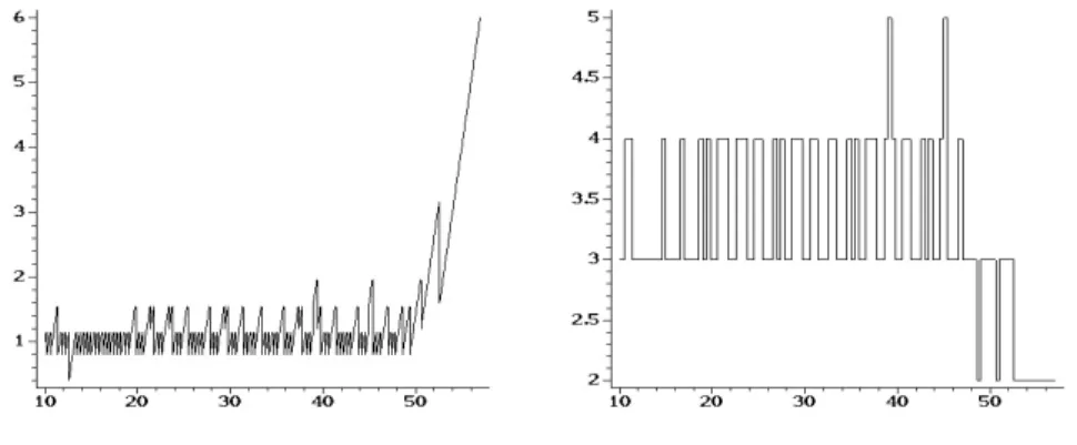
are the possible values of ∆ ρ we have not established their frequency for a given config-uration. The dead length is b= 12.6 and measurements for ρ between 2 and 68 will be obtained. We get 142 successive ρ that differs by 0.4, 2 that differs by 0.8, 1.2, 1.6 and 1 that differ by 2. The ∆ ρ distribution as a function of the cable length ρ is provided in figure 2. As may be seen, apart at the extremity, the ∆ ρ is everywhere equal to 0.4 with a mean value of 0.442 and a variance of 0.04571.
Let us now consider that dm= 1.3, dc= 2 so that dm/dc= 13/20 and kmax = 11.
We get the following pair (p/q, |∆ ρ|): (2/3, 0.1), (5/8, 0.4), (1/2, 0.6), (1/1, 0.7), (3/4, 0.8), (5/7, 0.9), (7/10, 1), (4/7, 1.1) and ∆ ρ= 0.1 may always be obtained . This is confirmed by the calculation with 216 measurement differing by 0.1, 72 by 0.4, 12 by 0.5, 12 by 0.6, 4 by 0.7 and 1 for 1.3. The value of b is 13.7 and we get measurements for ρ between 1.3 and 69 (figure 2). The mean value of the ∆ ρ is 0.213 and its variance is 0.0322. It may be observed that although we have almost doubled the number of
1A Farey sequence of order n are the irreducible rationals between 0 and 1 whose denominator
Fig. 2. On the left the distribution of ∆ ρ as a function of ρ for dm= 2.4, dc= 2 with 29 marks
and 6 color sensors. On the right the distribution for dm= 1.3, dc= 2 with 29 marks and 11 color
sensors.
color sensors compared to the previous case we still get a large number of cases with ∆ ρ= 0.4 so that the choice of dm= 1.3 may not be optimal. Optimal configuration is
addressed in the next section.
5.2 Optimal configuration
Optimal choice of sensor distance dmfor a given dc
A key point for realizing such a measurement system is first to determine what could be the number kmaxof color sensors and then select the dmfor the best performance. For
a given kmax, dmshould lie in the range]h/(kmax+1), h/kmax]. Consider for example that
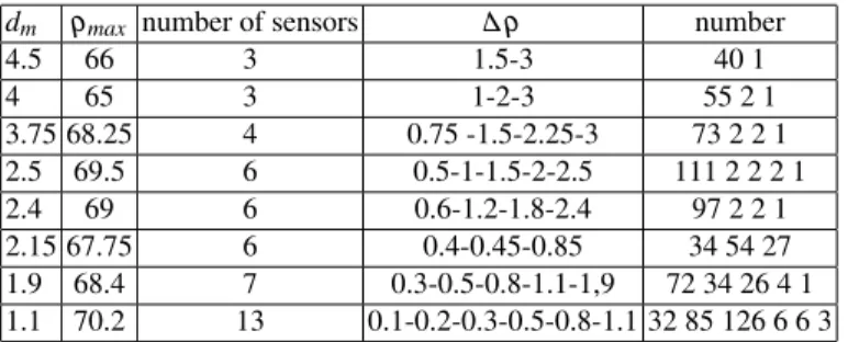
h= 15, kmax= 6, dc= 2. We may draw the curve of the mean and variance values of the
∆ ρ as a function of dm, figure 3. As may be seen the mean value of ∆ ρ is an increasing
function of dmwhile there is a discontinuity point for dm= 2.4 with a sudden increase
of the mean value but also a sudden decrease of the variance.
To understand this behavior we have to consider how many minimal ∆ ρ we will obtained for a given rational ratio dm/dc= p/q. For that purpose we have to look at
the rational p1/q1which has a denominator q1 lower or equal to kmax and that is the
closest to p/q. The larger the sets of possible k1, k are the larger will be the set of
minimal ∆ ρ. As the values of k1, k are restricted to lie respectively in the range[1, k1max−
p1],[1, kmax− q1] the larger the sets will be if p1, q1are close to 1.
Let us assume that q is lower than kmax. According to theorem 1 the closest rational
p1/q1that is lower than p/q should satisfy pp1− q1q= 1. If we set p1= q1= 1 we get
the constraint (A) p − q= 1 so that dm= pdc/(p − 1) Hence dmis a decreasing function
of p that cannot be greater than kmax= 6. If we look at all possible value for p between
1 and 6, then we found out that (A) may be satisfied only for p= 6. The corresponding dm/dcratio is 6/5= 2.4 and for this ratio we will get the maximal number of ∆ ρ that
Fig. 3. The mean value and variance of ∆ ρ as a function of the distance dmbetween the color
sensor for dc= 2 and 29 color marks
the mean value is not that good: other value of dmmay lead to a sequence of .∆ ρ whose
minimum is lower than 0.4.
Let us look now at dm= 2.35, a value that presents the second minimal value for
the variance. For this value we get 23 ∆ ρ= 0.25, 140 ∆ ρ = 0.35, 2 ∆ ρ = 0.6, 0.95, 1.3, 1.65 and 1 ∆ ρ= 2. Here we have a larger number of ∆ ρ equal to 0.25 or 0.35 than compared to the value 0.4 obtained for dm= 2.4. Hence apparently for a given dcwe
shall consider as possible optimal values of dmthe one having the lowest variances.
We may also consider increasing dcto a larger value for CDPR having large cable
length. For example if we have 29 marks with dc= 5, dm= 2.2 (6 sensors) we get a
measuring range of 151 meters with the following pairs of ∆ ρ and their number: (0.6, 112), (1, 27), (1.6, 30). If we move to dc= 10 and the same number of sensors and dm,
then the measuring range increases to 291 meters with (1, 28), (1.2, 56), (2.2, 88).
Influence of the number of marks
Although the number of sensors in a system is important, these sensors are inexpen-sive and require a low level of maintenance while the marks will require more attention. We may thus consider having less than the maximum number of marks imposed by the the initialization process, but this will impose to have larger dcin order to have a
suffi-cient total cable length.
As seen in the previous section the ratio dm/dc= p/q that has the maximum of
lowest ∆ ρ is such the closest rational with a denominator lower or equal to q should be p1/q1= 1/1. Using theorem 1 we get p − q = 1 if p1/q1 is lower than p/q so
that dm= dcp/(p − 1) provided that p − 1 is lower or equal to the number of sensors
f loor(h/dm). If p1/q1is greater than p/q we get q − p= 1 so that dm= dcp/(p + 1)
Assume that we will use only 20 marks instead of 29 but set dcto 3 in order to still
have a large total cable length. For dc= 3 table 1 provides some examples of dmleading
to interesting set of ∆ ρ with their distribution.
dm ρmax number of sensors ∆ ρ number 4.5 66 3 1.5-3 40 1 4 65 3 1-2-3 55 2 1 3.75 68.25 4 0.75 -1.5-2.25-3 73 2 2 1 2.5 69.5 6 0.5-1-1.5-2-2.5 111 2 2 2 1 2.4 69 6 0.6-1.2-1.8-2.4 97 2 2 1 2.15 67.75 6 0.4-0.45-0.85 34 54 27 1.9 68.4 7 0.3-0.5-0.8-1.1-1,9 72 34 26 4 1 1.1 70.2 13 0.1-0.2-0.3-0.5-0.8-1.1 32 85 126 6 6 3
Table 1. Minimal ∆ ρ measurement and their number for various dmbeing given dc= 3 and 20
marks on the cable
It may be seen that the best compromises for 3 sensors is dm= 4 with an increase
of accuracy for 4 sensors with dm = 3.75, while dm= 2.5 is optimal for 6 sensors.
Note that we have added a line with dm= 2.15 that correspond to the lowest variance
beside the one leading to the maximal number of minimal ∆ ρ as it offers interesting performances. As may be seen from this table increasing the number of sensors may have a large benefit on the measurement. For 13 sensors we get 243 changes for ∆ ρ in the range [0.1, 0.3].
We may now consider going into the opposite direction by increasing the number of marks in order to increase the accuracy of the system, at the price of requiring the reading of 4 marks to initialize the cable length (although this argument will be invali-dated if we use the initialization procedure described in section 5.3). Consider first that dc= 1.5 so that we have 40 marks. We consider the case where the variance is minimal
and table 2 summarizes the result. As it seems difficult to position the sensor with an
dm ρmax number of sensors ∆ ρ number 2.4 69.75 6 0.3-0.6-0.9-1.5 189 12 4 1 2.25 70.5 6 0.75-1.5 89 1 1.6875 70.3125 8 0.1875 . . . 305 1.8 71.1 8 0.3-0.6-0.9-1.2-1.5 209 2 2 2 1 1.83 71.31 8 0.15-0.18-0.33 . . . 102 140 69 1.66 71.78 9 0.16-0.22-. . . 312 31 1.35 72 11 0.15-. . . 392 1.27 71.2 11 0.11-0.12-0.23-. . . 136 175 118
Table 2. Minimal ∆ ρ measurement and their number for various dmbeing given dc= 1.5 and 40
accuracy of half a centimeter, the optimal solution for dmseem to be 2.4, 1.8, 1.83, 1.66,
1.35. Table 3 summarizes good design solutions for cable length in the range of 60-70 meters.
number of marks dc dm number of sensors ∆ ρ number 12 5 3.75 4 1.25 43 15 4 3 5 1 58 20 3 1 3 1 55 20 3 3.75 4 0.75 73 20 3 2.5 6 0.5 111 29 2 2.4 6 0.4 142 29 2 2.35 6 0.25-0.35 23-140 40 1.5 2.4 6 0.3-0.6 189-12 40 1.5 1.83 8 0.15-0.18-0.33 102-140-69 40 1.5 1.66 9 0.16-0.22 312-31 40 1.5 1.35 11 0.15 392 60 1 2.4 6 0.3 289 60 1 1.75 8 0.25 363 60 1 1.3 11 0.1 0.2 375 272 84 0.7 1 15 0.1 639
Table 3. Best system arrangement for various dc(distance between marks) and number of sensors
(dm= distance between color sensors)
5.3 The initialization problem: a second approach
We have proposed in section 3 a first approach to determine the initial cable length based on the detection of n successive marks by one sensor, the coding of the cable being such that there is a single occurrence of a given sequence of n colors on the cable. For the initialization process we therefore need to coil the cable by ndc. However we may get a
faster initialization process by taking into account that we have several color sensors in the mast so that we may use all event detection event for performing the initialization process. Clearly we aim at determining the cable length by coiling the cable by less than ndc.
If we have n different colors on the cable and m marks on the cable so that m is maximal, then we will have roughly m/n marks of the same color. For example for n= 3, m = 29 and the marking presented in section 3 we have 10 marks of color 1, 2 and 9 marks of color 3. Remind that if the color sensor ns detects mark ms, then the
cable length ρ is given by
ρ= nsdm− h + L0− (ms− 1)dc (6)
where L0is the total length of the cable. After starting the coiling there will be a first
color provides a limited choice for ms (at most 10 in our example) and consequently
a limited set {ρ1, . . . , ρl} of possible ρ. For each of the ρi we consider the set of all
possible values of ρ that are lower than ρi obtained for all possible values of ns, ms
and we then sort this set by decreasing value of ρ. The first element of the ordered set provides what will be the next sensor detection event if the current value of the ρ is ρi.
Hence we get a listL of (ρi, nis, ci) where nis is the sensor number and ciis the mark
color for the next event. When a new sensor event occurs we check the coherence of the nsand the color with each nis, ci: each element ofL that is not coherent with the
sensor number or color is removed fromL . This leads to a new list that contains all possible values of the current value of ρ and prediction about the next sensor event and we repeat the process. As the coherence test allows one to reduce the size ofL , we shall end up with a list with a single element that is the current value of ρ.
For example we consider the case where we have 29 marks separated by 2 meters with 3 different colors and 6 color sensors separated by 1.6 meter. If the cable length is ρ= 21.5 when starting the initialization process, then the first detection event is color 3 on sensor 4. Using color 3 we obtain the listL ={(45.4,5,1),(29.4,5,2),(21.4,5,2), (17.4, 5, 3), (15.4, 5, 1), (11.4, 5, 1), (3.4, 5, 3), (1.4, 5, 3)}. The second sensor event is color 2 for sensor 5 meaning that among the previous list only the value 21.4 and 29.4 are coherent, leading toL = {(29,6,2),(21,1,2)}. As the next event has color 2 and sensor 1 we may discard 29 and we will have determined that ρ= 20.2, after coiling only 1.3 meter of cable. More generally figures 4 shows how much cable should be coiled before getting the current ρ value as a function of the initial value of ρ and the number of detection events that are necessary to identify this value.
Fig. 4. On the left the coiling amount that is necessary to identify the current ρ as a function of the ρ value. On the right the number of sensor events that are necessary to identify the current ρ as a function of the ρ value (29 marks, 6 sensors, dc= 1.6, dm= 2).
As may be seen on these figures the average amount of coiling distance for the identification of the current ρ is 1.069 meter (variance: 0.054, min: 0.4, max: 1.95) for an initial ρ between 10 and 50 meter, much better than the value of 6 meters required
for the method proposed in section 3. If we use dm= 1.83, dc= 1.5, 8 color sensors and
40 marks, then in average we need only 0.622 meter of coiling (variance: 0.03, min: 0.34, max: 1.29) for determining the current ρ.
6
Conclusion
In this paper we propose a setup for both allowing an automated determination of the initial cable lengths and improving the cable length measurements. The method is sim-ple and allows one to obtain very good estimation of the current cable lengths especially for large CDPR (for example being able to provide the cable length for any change of 0.4 meter for a 60 meters cable). It allows also to get an estimate of the drum radius at each sensor event, thereby allowing to improve the estimation of the cable length between two sensor events. The method is robust: being given the sensor price it is pos-sible to use sever color sensors within a given sensor box. Furthermore it is pospos-sible to detect sensor failure based on the absence of a color signal during a significant change of cable length. We intend also to explore if this system may not allow to estimate the cable elastic deformation by comparing the difference between the distance between marks (that is known at rest) and the distance observed between sensor events. On-line calibration may also benefit from being able to fix the cable lengths at known values.
References
[Baczynski(2010)] Baczynski J, Baczynski M (2010) Simple system for determining starting position of cable-driven manipulator. In: IEEE Int. Conf. on Computer Information Systems and Industrial Management Applications (CISIM), Cracow, pp 102–106
[Bruijn(1946)] Bruijn N (1946) A combinatorial problem. Indagationes Math 8:461–467 [Bruijn(1975)] Bruijn N (1975) Acknowledgment of priority to c. flye sainte-marie on the
count-ing of circular arrangements of 2nzeros and ones that show each n-letter word exactly once. Indhove: Technische Hogeschool Eidenhoven
[Chen(2004)] Chen Q, et al (2004) An integrated two-level self-calibration method for cable-driven manipulator. IEEE Trans on Robotics 10(2):380–391
[Gouttefarde et al(2012)] Gouttefarde M, et al (2012) Simplified static analysis of large-dimension parallel cable-driven robots. In: IEEE Int. Conf. on Robotics and Automation, Saint Paul, pp 2299–2305
[Merlet(2008)] Merlet JP (2008) Kinematics of the wire-driven parallel robot MARIONET using linear actuators. In: IEEE Int. Conf. on Robotics and Automation, Pasadena
[Merlet(2010)] Merlet JP (2010) MARIONET, a family of modular wire-driven parallel robots. In: ARK, Piran, pp 53–62
[Miermeister and Pott(2012)] Miermeister P, Pott A (2012) Auto calibration method for cable-driven parallel robot using force sensors. In: ARK, Innsbruck, pp 269–276
[Pott et al(2012)] Pott A, et al (2012) IPAnema: a family of cable-driven parallel robots for in-dustrial applications. In: 1st Int. Conf. on cable-driven parallel robots (CableCon), Stuttgart, pp 119–134
[Alexandre(2012)] Alexandre dit Sandretto J, Daney D, Gouttefarde M (2012) Calibration of a fully-constrained parallel cable-driven robot. In: RoManSy, Paris, pp 12–41
[Alexandre et al(2013)] Alexandre dit Sandretto J, et al (2013) Certified calibration of a cable-driven robot using interval contractor programming. In: Computational Kinematics, Barcelona