HAL Id: hal-03245525
https://hal.archives-ouvertes.fr/hal-03245525
Submitted on 2 Jun 2021
HAL is a multi-disciplinary open access
archive for the deposit and dissemination of
sci-entific research documents, whether they are
pub-lished or not. The documents may come from
teaching and research institutions in France or
abroad, or from public or private research centers.
L’archive ouverte pluridisciplinaire HAL, est
destinée au dépôt et à la diffusion de documents
scientifiques de niveau recherche, publiés ou non,
émanant des établissements d’enseignement et de
recherche français ou étrangers, des laboratoires
publics ou privés.
silicon in the modern ocean
Paul Tréguer, Jill Sutton, Mark Brzezinski, Matthew A. Charette, Timothy
Devries, Stephanie Dutkiewicz, Claudia Ehlert, Jon Hawkings, Aude
Leynaert, Su Mei Liu, et al.
To cite this version:
Paul Tréguer, Jill Sutton, Mark Brzezinski, Matthew A. Charette, Timothy Devries, et al.. Reviews
and syntheses: The biogeochemical cycle of silicon in the modern ocean. Biogeosciences, European
Geosciences Union, 2021, 18 (4), pp.1269–1289. �10.5194/bg-18-1269-2021�. �hal-03245525�
https://doi.org/10.5194/bg-18-1269-2021 © Author(s) 2021. This work is distributed under the Creative Commons Attribution 4.0 License.
Reviews and syntheses: The biogeochemical cycle of silicon
in the modern ocean
Paul J. Tréguer1,2, Jill N. Sutton1, Mark Brzezinski3, Matthew A. Charette4, Timothy Devries5, Stephanie Dutkiewicz6, Claudia Ehlert7, Jon Hawkings8,9, Aude Leynaert1, Su Mei Liu10,11,
Natalia Llopis Monferrer1, María López-Acosta12,13, Manuel Maldonado13, Shaily Rahman14, Lihua Ran15, and Olivier Rouxel16
1Univ Brest, CNRS, IRD, Ifremer, Institut Universitaire Européen de la Mer, LEMAR, Rue Dumont d’Urville,
29280, Plouzané, France
2State Key Laboratory of Satellite Ocean Dynamics (SOED), Ministry of Natural Resource, Hangzhou 310012, China 3Marine Science Institute, University of California, Santa Barbara, CA, USA
4Department of Marine Chemistry and Geochemistry, Woods Hole Oceanographic Institution, Woods Hole, MA 02543, USA 5Department of Geography, University of California, Santa Barbara, CA, USA
6Department of Earth, Atmospheric and Planetary Sciences (DEAPS), Massachusetts Institute of Technology (MIT),
Cambridge, MA 02139, USA
7Research Group for Marine Isotope Geochemistry, Institute for Chemistry and Biology of the Marine Environment (ICBM),
Carl von Ossietzky University of Oldenburg, Oldenburg, Germany
8National High Magnetic Field Lab and Earth, Ocean and Atmospheric Sciences, Florida State University, Tallahassee, USA 9Interface Geochemistry, German Research Centre for Geosciences GFZ, Potsdam, Germany
10Frontiers Science Center for Deep Ocean Multispheres and Earth System, and Laboratory of Marine Chemistry Theory and
Technology MOEy, Ocean University of China, Qingdao 266100, China
11Laboratory for Marine Ecology and Environmental Science, Qingdao National Laboratory for Marine Science and
Technology, Qingdao 266237, China
12Institute of Marine Research (IIM-CSIC), Rúa de Eduardo Cabello 6, Vigo 36208, Pontevedra, Spain
13Department of Marine Ecology. Center for Advanced Studies of Blanes (CEAB-CSIC), Acceso Cala St. Francesc 14,
Blanes 17300, Girona, Spain
14School of Ocean Science and Engineering, University of Southern Mississippi, Stennis Space Center, MS 39529, USA 15Key Laboratory of Marine Ecosystem Dynamics, Second Institute of Oceanography,
Ministry of Natural Resources, P. R. China
16IFREMER, Centre de Brest, Technopôle Brest Iroise, Plouzané, France
Correspondence: Paul Tréguer (paul.treguer@univ-brest.fr) and Jill Sutton (jill.sutton@univ-brest.fr) Received: 20 July 2020 – Discussion started: 3 August 2020
Revised: 18 December 2020 – Accepted: 23 December 2020 – Published: 18 February 2021
Abstract. The element silicon (Si) is required for the growth of silicified organisms in marine environments, such as di-atoms. These organisms consume vast amounts of Si to-gether with N, P, and C, connecting the biogeochemical cy-cles of these elements. Thus, understanding the Si cycle in the ocean is critical for understanding wider issues such as carbon sequestration by the ocean’s biological pump. In this review, we show that recent advances in process studies
in-dicate that total Si inputs and outputs, to and from the world ocean, are 57 % and 37 % higher, respectively, than previ-ous estimates. We also update the total ocean silicic acid in-ventory value, which is about 24 % higher than previously estimated. These changes are significant, modifying factors such as the geochemical residence time of Si, which is now about 8000 years, 2 times faster than previously assumed. In addition, we present an updated value of the global
an-nual pelagic biogenic silica production (255 Tmol Si yr−1) based on new data from 49 field studies and 18 model outputs, and we provide a first estimate of the global an-nual benthic biogenic silica production due to sponges (6 Tmol Si yr−1). Given these important modifications, we hypothesize that the modern ocean Si cycle is at approxi-mately steady state with inputs = 14.8(±2.6) Tmol Si yr−1 and outputs = 15.6(±2.4) Tmol Si yr−1. Potential impacts of global change on the marine Si cycle are discussed.
1 Introduction
Silicon, the seventh most abundant element in the universe, is the second most abundant element in the Earth’s crust. The weathering of the Earth’s crust by CO2-rich rainwater,
a key process in the control of atmospheric CO2(Berner et
al., 1983; Wollast and Mackenzie, 1989), results in the gen-eration of silicic acid (dSi; Si(OH)4) in aqueous
environ-ments. Silicifiers are among the most important aquatic or-ganisms and include micro-oror-ganisms (e.g., diatoms, rhizar-ians, silicoflagellates, several species of choanoflagellates) and macro-organisms (e.g., siliceous sponges). Silicifiers use dSi to precipitate biogenic silica (bSi; SiO2) as internal
(Moriceau et al., 2019) and/or external (Maldonado et al., 2019) structures. Phototrophic silicifiers, such as diatoms, globally consume vast amounts of Si concomitantly with ni-trogen (N), phosphorus (P), and inorganic carbon (C), con-necting the biogeochemistry of these elements and contribut-ing to the sequestration of atmospheric CO2 in the ocean
(Tréguer and Pondaven, 2000). Heterotrophic organisms like rhizarians, choanoflagellates, and sponges produce bSi in-dependently of the photoautotrophic processing of C and N (Maldonado et al., 2012, 2019; Llopis Monferrer et al., 2020).
Understanding the Si cycle is critical for understanding the functioning of marine food webs, biogeochemical cy-cles, and the biological carbon pump. Herein, we review re-cent advances in field observations and modeling that have changed our understanding of the global Si cycle and provide an update of four of the six net annual input fluxes and of all the output fluxes previously estimated by Tréguer and De La Rocha (2013). Taking into account numerous field studies in different marine provinces and model outputs, we re-estimate the Si production (Nelson et al., 1995), review the potential contribution of rhizarians (Llopis Monferrer et al., 2020) and picocyanobacteria (Ohnemus et al., 2016), and give an esti-mate of the total bSi production by siliceous sponges using recently published data on sponge bSi in marine sediments (Maldonado et al., 2019). We discuss the question of the bal-ance and imbalbal-ance of the marine Si biogeochemical cycle at different timescales, and we hypothesize that the mod-ern ocean Si cycle is potentially at steady state with inputs =14.8(±2.6) Tmol Si yr−1approximately balancing outputs
=15.6(±2.4) Tmol Si yr−1(Fig. 1). Finally, we address the question of the potential impact of anthropogenic activities on the global Si cycle and suggest guidelines for future re-search endeavors.
2 Advances in input fluxes
Silicic acid is delivered to the ocean through six pathways as illustrated in Fig. 1, which all ultimately derive from the weathering of the Earth’s crust (Tréguer and De La Rocha, 2013). All fluxes are given with an error of 1 standard devia-tion.
2.1 Riverine (FR) and aeolian (FA) contributions
The best estimate for the riverine input (FR) of dSi, based
on data representing 60 % of the world river discharge and a discharge-weighted average dSi riverine concentra-tion of 158 µM − Si (Dürr et al., 2011), remains at FRdSi=
6.2(±1.8) Tmol Si yr−1 (Tréguer and De La Rocha, 2013). However, not only dSi is transferred from the terrestrial to the riverine system, with particulate Si mobilized in crys-tallized or amorphous forms (Dürr et al., 2011). Accord-ing to Saccone et al. (2007), the term “amorphous silica” (aSi) includes biogenic silica (bSi, from phytoliths, fresh-water diatoms, sponge spicules), altered bSi, and pedogenic silicates, the three of which can have similar high solubili-ties and reactivisolubili-ties. Delivery of aSi to the fluvial system has been reviewed by Frings et al. (2016), and they suggested a value of FRaSi=1.9(±1.0) Tmol Si yr−1. Therefore, total
FR=8.1(±2.0) Tmol Si yr−1.
No progress has been made regarding aeolian dust depo-sition into the ocean (Tegen and Kohfeld, 2006) and subse-quent release of dSi via dust dissolution in seawater since Tréguer and De La Rocha (2013), who summed the flux of particulate dissolvable silica and wet deposition of dSi through precipitation. Thus, our best estimate for the aeolian flux of dSi, FA, remains 0.5(±0.5) Tmol Si yr−1.
2.2 Dissolution of minerals (FW)
As shown in Fig. 2, the low-temperature dissolution of siliceous minerals in seawater and from sediments feeds a dSi flux, FW, through two processes: (1) the dissolution of
river-derived lithogenic particles deposited along the conti-nental margins and shelves and (2) the dissolution of basaltic glass in seawater, processes that work mostly in deep waters. About 15–20 Gt yr−1of river-derived lithogenic particles are deposited along the margins and shelves (e.g., Syvitskia et al., 2003; also see Fig. 2). Dissolution experiments with river sediments or basaltic glass in seawater showed that 0.08 %– 0.17 % of the Si in the solid phase was released within a few days to months (e.g., Oelkers et al., 2011; Jones et al., 2012; Pearce et al., 2013; Morin et al., 2015). However, the high solid-to-solution ratios in these experiments increased
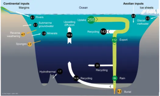
Figure 1. Schematic view of the Si cycle in the modern world ocean (input, output, and biological Si fluxes), and possible balance (total Si inputs = total Si outputs = 15.6 Tmol Si yr−1) in reasonable agreement with the individual range of each flux (F ); see Tables 1 and 2. The white arrows represent fluxes of net sources of silicic acid (dSi) and/or of dissolvable amorphous silica (aSi) and of dSi recycled fluxes. Orange arrows correspond to sink fluxes of Si (either as biogenic silica or as authigenic silica). Green arrows correspond to biological (pelagic) fluxes. All fluxes are in teramoles of silicon per year (Tmol Si yr−1). Details are given in Sect. S1 in the Supplement.
the dSi concentration quickly to near-equilibrium conditions inhibiting further dissolution, which prevents direct compar-ison with natural sediments. Field observations and subse-quent modeling of Si release range around 0.5 %–5 % yr−1 of the Si originally present in the solid phase dissolved into the seawater (e.g., Arsouze et al., 2009; Jeandel and Oelkers, 2015). On the global scale, Jeandel et al. (2011) estimated the total flux of dissolution of minerals to range between 0.7– 5.4 Tmol Si yr−1, i.e., similar to the dSi river flux. However, this estimate is based on the assumption of 1 %–3 % congru-ent dissolution of sedimcongru-ents for a large range of lithological composition which, so far, has not been proven.
Another approach to estimate FW is to consider the
ben-thic efflux from sediments devoid of biogenic silica deposits. Frings (2017) estimates that “non-biogenic-silica” sediments (i.e., clays and calcareous sediments, which cover about 78 % of the ocean area) may contribute up to 44.9 Tmol Si yr−1via a benthic diffusive Si flux. However, according to lithological descriptions given in GSA Data Repository 2015271 some of the non-biogenic-silica sediment classes described in this study may contain significant bSi, which might explain this high estimate for FW. Tréguer and De La Rocha (2013)
con-sidered benthic efflux from non-siliceous sediments ranging between ≈ 10–20 mmol m−2yr−1in agreement with Tréguer et al. (1995). If extrapolated to the 120 million square kilo-meter zone of opal-poor sediments in the global ocean, this gives an estimate of FW=1.9(±0.7) Tmol Si yr−1.
2.3 Submarine groundwater (FGW)
Since 2013, several papers have sought to quantify the global oceanic input of dissolved Si (dSi) from submarine ground-water discharge (SGD), which includes terrestrial (freshwa-ter) and marine (saltwa(freshwa-ter) components (Fig. 2). Silicic acid inputs through SGD may be considerable, similar to or in ex-cess of riverine input in some places. For instance, Georg et al. (2009) estimated this input to be 0.093 Tmol Si yr−1in the Bay of Bengal, which is ≈ 66 % of the Ganges–Brahmaputra river flux of dSi to the ocean. At a global scale the best es-timate of Tréguer and De La Rocha (2013) for FGW was
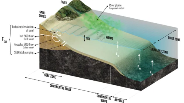
0.6(±0.6) Tmol Si yr−1. More recently, Rahman et al. (2019) used a global terrestrial SGD flux model weighted accord-ing to aquifer lithology (Beck et al., 2013) in combination with a compilation of dSi in shallow water coastal aquifers to derive a terrestrial groundwater input of dSi to the world ocean of 0.7(±0.1) Tmol Si yr−1. This new estimate, with its relatively low uncertainty, represents the lower limit flux of dSi to the ocean via SGD. The marine component of SGD, driven by a range of physical processes such as density gra-dients or waves and tides, is fed by seawater that circulates through coastal aquifers or beaches via advective flow paths (Fig. 2; also see Fig. 1 of Li et al., 1999). This circulating seawater may become enriched in dSi through bSi or min-eral dissolution, the degree of enrichment being determined by subsurface residence time and mineral type (Techer et al., 2001; Anschutz et al., 2009; Ehlert et al. 2016a).
Several lines of evidence show that the mineral dissolu-tion (strictly corresponding to net dSi input) may be
sub-Figure 2. Schematic view of the low-temperature processes that control the dissolution of (either amorphous or crystallized) siliceous minerals in seawater in and to the coastal zone and in the deep ocean, feeding FGWand FW. These processes correspond to both low and medium energy flux dissipated per volume of a given siliceous particle in the coastal zone, in the continental margins, and in the abysses and to high-energy flux dissipated in the surf zone. Details are given in S1 in the Supplement.
stantial (e.g., Ehlert et al., 2016b). Focusing on processes occurring in tidal sands, Anschultz et al. (2009) showed that they can be a biogeochemical reactor for the Si cy-cle. Extrapolating laboratory-based dissolution experiments performed with pure quartz, Fabre et al. (2019) calcu-lated the potential flux of dissolution of siliceous sandy beaches that is driven by wave and tidal action. If, ac-cording to Luijendijk et al. (2018) one-third of the world’s shorelines are sandy beaches, this dissolution flux could be 3.2(±1.0) Tmol Si yr−1. However, this estimate is not well constrained because it has not been validated by field ex-periments (Sect. S2 in the Supplement). Cho et al. (2018), using a228Ra inverse model and groundwater dSi/228Ra ra-tios, estimate the total (terrestrial + marine) SGD dSi flux to the ocean to be 3.8(±1.0) Tmol Si yr−1; this represents an upper limit value for SGD’s contribution to the global ocean dSi cycle. Without systematic data that corroborate the net input of dSi through the circulation of the marine component of SGD (e.g., porewater δ30Si, paired dSi and
228Ra measurements), we estimate the range of net input of
dSi through total SGD as 0.7 Tmol Si yr−1(Rahman et al., 2019) to 3.8 Tmol Si yr−1(Cho et al., 2018), with an average, i.e., FGW=2.3(±1.1) Tmol Si yr−1, which is approximately
3 times larger than that of Tréguer and De La Rocha (2013). 2.4 (Sub)polar glaciers (FISMW)
This flux was not considered by Tréguer and De La Rocha (2013). Several researchers have now identified polar
glaciers as sources of Si to marine environments (Tréguer, 2014; Meire et al., 2016; Hawkings et al., 2017). The cur-rent best estimate of discharge-weighted dSi concentration in (sub)Arctic glacial meltwater rivers lies between 20–30 µM, although concentrations ranging between 3 and 425 µM have been reported (Graly et al., 2014; Meire et al., 2016; Hat-ton et al., 2019). Only two values currently exist for dSi from subglacial meltwater beneath the Antarctic Ice Sheet (Whillans subglacial lake and Mercer subglacial lake, 126– 140 µM; Michaud et al., 2016, Hawkings et al., 2020), and there is a limited dataset from periphery glaciers in the Mc-Murdo Dry Valleys and Antarctic Peninsula (≈ 10–120 µM; Hatton et al., 2020; Hirst et al., 2020). Furthermore, ice-berg dSi concentrations remain poorly quantified but are ex-pected to be low (≈ 5 µM; Meire et al., 2016). Meltwater typically contains high suspended sediment concentrations, due to intense physical erosion by glaciers, with a relatively high dissolvable aSi component (0.3 %–1.5 % dry weight) equating to concentrations of 70–340 µM (Hawkings et al., 2018; Hatton et al., 2019). Iceberg aSi concentrations are lower (28–83 µM) (Hawkings et al., 2017). This particu-late phase appears fairly soluble in seawater (Hawkings et al., 2017), and large benthic dSi fluxes in glacially influ-enced shelf seas have been observed (Hendry et al., 2019; Ng et al., 2020). Direct silicic acid input from (sub)polar glaciers is estimated to be 0.04(±0.04) Tmol Si yr−1. If the aSi flux is considered then this may provide an ad-ditional 0.29(±0.22) Tmol Si yr−1, with a total FISMW (=
dSi + aSi) input estimate of 0.33(±0.26) Tmol Si yr−1. This does not include any additional flux from benthic process-ing of glacially derived particles in the coastal regions (see Sect. 2.2 above).
2.5 Hydrothermal activity (FH)
The estimate of Tréguer and De La Rocha (2013) for FH
was 0.6(±0.4) Tmol Si yr−1. Seafloor hydrothermal activity at mid-ocean ridges (MORs) and ridge flanks is one of the fundamental processes controlling the exchange of heat and chemical species between seawater and ocean crust (Wheat and Mottl, 2000). A major challenge limiting our current models of both heat and mass flux (e.g., Si flux) through the seafloor is estimating the distribution of the various forms of hydrothermal fluxes, including focused (i.e., high temper-ature) vs. diffuse (i.e., low tempertemper-ature) and ridge axis vs. ridge flank fluxes. Estimates of the Si flux for each input are detailed below.
Axial and near-axial hydrothermal flux settings. The best estimate of the heat flux at ridge axis (i.e., crust 0–0.1 Ma in age) is 1.8(±0.4) TW, while the heat flux in the near-axial region (i.e., crust 0.1–1 Ma in age) has been inferred at 1.0(±0.5) TW (Mottl, 2003). The con-version of heat flux to hydrothermal water and chemical fluxes requires assumptions regarding the temperature at which this heat is removed. For an exit temperature of 350(±30)◦C typical of black smoker vent fluids, and an as-sociated enthalpy of 1500(±190) J g−1at 450–1000 bar and heat flux of 2.8(±0.4) TW, the required seawater flux is 5.9(±0.8)×1016g yr−1(Mottl, 2003). High-temperature hy-drothermal dSi flux is calculated using a dSi concentration of 19(±11) mmol kg−1, which is the average concentration in hydrothermal vent fluids that have an exit temperature > 300◦C (Mottl, 2012). This estimate is based on a compila-tion of > 100 discrete vent fluid data, corrected for seawater mixing (i.e., end-member values at Mg = 0; Edmond et al., 1979) and phase separation. Although the chlorinity of hot springs varies widely, nearly all of the reacted fluid, whether vapor or brine, must eventually exit the crust within the ax-ial region. The integrated hot spring flux must therefore have a chlorinity similar to that of seawater. The relatively large range of dSi concentrations in high-temperature hydrother-mal fluids likely reflect the range of geological settings (e.g., fast- and slow-spreading ridges) and host-rock composition (ultramafic, basaltic, or felsic rocks). Because dSi enrich-ment in hydrothermal fluids results from mineral–fluid in-teractions at depth and is mainly controlled by the solubil-ity of secondary minerals such as quartz (Mottl 1983; Von Damm et al. 1991), it is also possible to obtain a theoretical estimate of the concentration of dSi in global hydrothermal vent fluids. Under the conditions of temperature and pres-sure (i.e., depth) corresponding to the base of the upflow zone of high temperature (> 350–450◦C) hydrothermal sys-tems, dSi concentrations between 16 and 22 mmol kg−1 are
calculated, which is in good agreement with measured values in end-member hydrothermal fluids. Using a dSi concentra-tion of 19(±3.5) mmol kg−1and water flux of 4.8(±0.8) × 1016g yr−1, we determine an axial hydrothermal Si flux of 0.91(±0.29) Tmol Si yr−1. It should be noted, however, that high-temperature hydrothermal fluids may not be entirely responsible for the transport of all the axial hydrothermal heat flux (Elderfield and Schultz, 1996; Nielsen et al., 2006). Because dSi concentrations in diffuse hydrothermal fluids are not significantly affected by subsurface Si precipitation during cooling of the hydrothermal fluid (Escoube et al., 2015), we propose that the global hydrothermal Si flux is not strongly controlled by the nature (focused vs. diffuse) of ax-ial fluid flow.
Ridge flank hydrothermal fluxes.Chemical fluxes related to seawater–crust exchange at ridge flanks have been previ-ously determined through direct monitoring of fluids from low-temperature hydrothermal circulation (Wheat and Mottl, 2000). Using basaltic formation fluids from the 3.5 Ma crust on the eastern flank of the Juan de Fuca Ridge (Wheat and McManus, 2005), a global flux of 0.011 Tmol Si yr−1 for the warm ridge flank is calculated. This estimate is based on the measured Si anomaly associated with warm spring (0.17 mmol kg−1) and a ridge flank fluid flux determined using oceanic Mg mass balance, therefore assuming that the ocean is at steady state with respect to Mg. More re-cent results of basement fluid compositions in cold and oxy-genated ridge flank settings (e.g., North Pond, Mid-Atlantic Ridge) also confirm that incipient alteration of volcanic rocks may result in significant release of Si to circulating seawa-ter (Meyer et al., 2016). The total heat flux through ridge flanks, from 1 Ma crust to a sealing age of 65 Ma, has been estimated at 7.1(±2) TW. Considering that most of ridge flank hydrothermal power output should occur at cool sites (< 20◦C), the flux of slightly altered seawater could range from 0.2 to 2 × 10¹⁹g yr−1, rivaling the flux of river water to the ocean of 3.8 × 10¹⁹g yr−1(Mottl, 2003). Using this esti-mate and Si anomaly of 0.07 mmol−Si kg−1reported in cold ridge flank setting from North Pond (Meyer et al., 2016), a Si flux of 0.14 to 1.4 Tmol Si yr−1for the cold ridge flank could be calculated. Because of the large volume of seawater interacting with oceanic basalts in ridge flank settings, even a small chemical anomaly resulting from reactions within these cold systems could result in a globally significant el-emental flux. Hence, additional studies are required to better determine the importance of ridge flanks to oceanic Si bud-get.
Combining axial and ridge flank estimates, the best esti-mate for FHis now 1.7(±0.8) Tmol Si yr−1, approximately 3
times larger than the estimate from Tréguer and De La Rocha (2013).
2.6 Total net inputs (Table 1A)
Total Si input = 8.1(±2.0)(FR(dSi+aSi)) +0.5(±0.5)(FA) +
1.9(±0.7)(FW) +2.3(±1.1)(FGW) +0.3(±0.3)(FISMW) +
1.7(±0.8)(FH) =14.8(±2.6) Tmol Si yr−1.
The uncertainty of the total Si inputs (and total Si out-puts, Sect. 3) has been calculated using the error propaga-tion method from Bevington and Robinson (2003). This has been done for both the total fluxes and the individual flux estimates.
3 Advances in output fluxes
3.1 Long-term burial of planktonic biogenic silica in sediments (FB)
Long-term burial of bSi, which generally occurs below the top 10–20 cm of sediment, was estimated by Tréguer and De La Rocha (2013) to be 6.3(±3.6) Tmol Si yr−1. The burial rates are highest in the Southern Ocean (SO), the North Pa-cific Ocean, the equatorial PaPa-cific Ocean, and the coastal and continental margin zone (CCMZ; DeMaster, 2002; Hou et al., 2019; Rahman et al., 2017).
Post-depositional redistribution by processes like win-nowing or focusing by bottom currents can lead to under-and over-estimation of uncorrected sedimentation under-and burial rates. To correct for these processes, the burial rates are typ-ically normalized using the particle reactive nuclide 230Th method (e.g., Geibert et al., 2005). A230Th normalization of bSi burial rates has been extensively used for the SO (Tréguer and De La Rocha, 2013), particularly in the “opal belt” zone (Pondaven et al., 2000; DeMaster, 2002; Geibert et al., 2005). Chase et al. (2015) re-estimated the SO burial flux, south of 40◦S at 2.3(±1.0) Tmol Si yr−1.
Hayes et al. (2020, 2021) recently calculated total ma-rine bSi burial of 5.46(±1.18) Tmol Si yr−1, using a database that comprises 2948 bSi concentrations of top core sediments and230Th-corrected accumulation fluxes of open-ocean loca-tions > 1 km in depth. The230Th-corrected total burial rate of Hayes et al. (2021) is 2.68(±0.61) Tmol Si yr−1south of 40◦S, close to the estimate of Chase et al. (2015) for the SO. Hayes et al. (2021) do not distinguish between the dif-ferent analytical methods used for the determination of the bSi concentrations of these 2948 samples to calculate total bSi burial. These methods include alkaline digestion meth-ods (with variable protocols for correcting from lithogenic interferences; e.g., DeMaster, 1981; Mortlock and Froelich, 1989; Müller and Schneider, 1993), X-ray diffraction (e.g., Leinen et al., 1986), X-ray fluorescence (e.g., Finney et al., 1988), Fourier-transform infrared spectroscopy (Lippold et al., 2012), and inductively coupled plasma mass spectrome-try (e.g., Prakash Babu et al., 2002). An international exer-cise calibration on the determination of bSi concentrations of various sediments (Conley, 1998) concluded that the
X-ray diffraction (XRD) method generated bSi concentrations that were on average 24 % higher than the alkaline digestion methods. In order to test the influence of the XRD method on their re-estimate of total bSi burial, Hayes et al. (2021) found that their re-estimate (5.46(±1.18) Tmol Si yr−1), which in-cludes XRD data (≈ 40 % of the total number of data points), did not differ significantly from a re-estimate that does not include XRD data points (5.43(±1.18) Tmol Si yr−1). As a result, this review includes the re-estimate of Hayes et al. (2021) for the open-ocean annual burial rate, i.e., 5.5(±1.2) Tmol Si yr−1.
The best estimate for the open-ocean total burial now becomes 2.8(±0.6) Tmol Si yr−1 without the SO contribu-tion (2.7(±0.6) Tmol Si yr−1). This value is an excess of 1.8 Tmol Si yr−1over the DeMaster (2002) and Tréguer and De La Rocha (2013) estimates, which were based on 31 sed-iment cores mainly distributed in the Bering Sea, the North Pacific, the Sea of Okhotsk, and the equatorial Pacific (to-tal area 23 million square kilometers) and where bSi % was determined solely using alkaline digestion methods.
Estimates of the silica burial rates have usually been de-termined from carbon burial rates using a Si : C ratio of 0.6 in CCMZ (DeMaster 2002). However, we now have inde-pendent estimates of marine organic C and total initial bSi burial (e.g., Aller et al., 1996, 2008; Galy et al., 2007; Rah-man et al., 2016, 2017). It has been shown that the initial bSi burial in sediment evolved as unaltered bSi or as au-thigenically formed aluminosilicate phases (Rahman et al., 2017). The Si : C burial ratios of residual marine plankton post-remineralization in tropical and subtropical deltaic sys-tems are much greater (2.4–11) than the 0.6 Si : C burial ratio assumed for continental margin deposits (DeMaster, 2002). The sedimentary Si : C preservation ratios are therefore sug-gested to depend on differential remineralization pathways of marine bSi and Corg under different diagenetic regimes
(Aller, 2014). Partitioning of32Si activities between bSi and mineral pools in tropical deltaic sediments indicate rapid and near-complete transformation of initially deposited bSi to au-thigenic clay phases (Rahman et al., 2017). For example, in subtropical/temperate deltaic and estuarine deposits,32Si ac-tivities represent approximately ≈ 50 % of initial bSiopal
de-livery to sediments (Rahman et al., 2017). Using the 32Si technique, Rahman et al. (2017) provided an updated esti-mate of bSi burial for the CCMZ of 3.7(±2.1) Tmol Si yr−1, higher than the Tréguer and De La Rocha (2013) estimate of 3.3(±2.1) Tmol Si yr−1based on the Si : C method of De-Master (2002).
Combining the Hayes et al. (2021) burial rate for the open-ocean zone including the SO and the Rahman et al. (2017) es-timate for the CCMZ gives a revised global total burial flux, FB, of 9.2(±1.6) Tmol Si yr−1, 46 % larger than the Tréguer
3.2 Deposition and long-term burial of sponge silica (FSP)
The estimate of Tréguer and De La Rocha (2013) for FSP,
the net sink of sponge bSi in sediments of continental mar-gins, was 3.6(±3.7) Tmol Si yr−1. The longevity of sponges, ranging from years to millennia, temporally decouples the process of skeleton production from the process of deposi-tion to the sediments (Jochum et al., 2017). While sponges slowly accumulate bSi over their long and variable lifetimes (depending on the species), the deposition to the sediments of the accumulated bSi is a relatively rapid process after sponge death, lasting days to months (Sect. S3 in the Supplement). The estimate of Tréguer and De La Rocha (2013) was cal-culated as the difference between the sponge dSi demand on continental shelves (3.7(±3.6) Tmol Si yr−1) – estimated from silicon consumption rates available for a few sublittoral sponge species (Maldonado et al., 2011) – and the flux of dSi from the dissolution of sponge skeletons in continen-tal shelves (0.15(±0.15) Tmol Si yr−1). This flux was tenta-tively estimated from the rate of dSi dissolution from a rare, unique glass sponge reef in British Columbia (Canada; Chu et al., 2011) and which is unlikely to be representative of the portion of sponge bSi that dissolves back as dSi after sponge death and before their burial in the sediments. To improve the estimate, Maldonado et al. (2019) used microscopy to access the amount of sponge silica that was actually being buried in the marine sediments using 17 sediment cores representing different marine environments. The deposition of sponge bSi was found to be 1 order of magnitude more intense in sed-iments of continental margins and seamounts than on conti-nental rises and central basin bottoms. The new best estimate for FSPis 1.7(±1.6) Tmol Si yr−1, assuming that the rate of
sponge silica deposition in each core was approximately con-stant through the Holocene, i.e., 2 times smaller than Tréguer and De La Rocha’s preliminary estimate.
3.3 Reverse weathering flux (FRW)
The previous estimate for this output flux, pro-vided by Tréguer and De La Rocha (2013), FRW=
1.5(±0.5) Tmol Si yr−1, was determined using indirect evidence since the influence of reverse weathering on the global Si cycle prior to 2013 was poorly understood. For example, reverse weathering reactions at the sediment–water interface were previously thought to constitute a relatively minor sink (0.03–0.6 Tmol Si yr−1) of silica in the ocean (DeMaster, 1981). The transformation of bSi to a neoformed aluminosilicate phase, or authigenic clay formation, was assumed to proceed slowly (> 104–105 years) owing prin-cipally to the difficulty of distinguishing the contribution of background lithogenic or detrital clays using the common leachates employed to quantify bSi (DeMaster, 1981). Recent direct evidence supporting the rapid formation of authigenic clays comes from tropical and subtropical deltas
(Michalopoulos and Aller, 1995; Rahman et al., 2016, 2017; Zhao et al., 2017), and several geochemical tools show that authigenic clays may form ubiquitously in the global ocean (Michalopoulos and Aller, 2004; Ehlert et al., 2016a; Baronas et al., 2017; Geilert et al., 2020; Pickering et al., 2020). Activities of cosmogenic 32Si (t1/2≈140 years),
incorporated into bSi in the surface ocean, provide demon-strable proof of rapid reverse weathering reactions by tracking the fate of bSi upon delivery to marine sediments (Rahman et al., 2016). By differentiating sedimentary bSi storage between unaltered bSi (bSiopal) and diagenetically
altered bSi (bSialtered) in the proximal coastal zone, 32Si
activities in these pools indicate that 3.7 Tmol Si yr−1 is buried as unaltered bSiopal and 4.7(±2.3) Tmol Si yr−1 as
authigenic clays (bSiclay) on a global scale. Here, we adopt
4.7 Tmol Si yr−1 for FRW representing about 3 times the
value of Tréguer and De La Rocha (2013). 3.4 Total net output (Table 1A)
Total Si output = 9.2 (± 1.6) (FB(net deposit)) + 4.7 (± 2.3)
(FRW) + 1.7 (± 1.6) (FSP) = 15.6 (± 2.4) Tmol Si yr−1.
4 Advances in biological fluxes 4.1 Annual bSi pelagic production 4.1.1 From field data
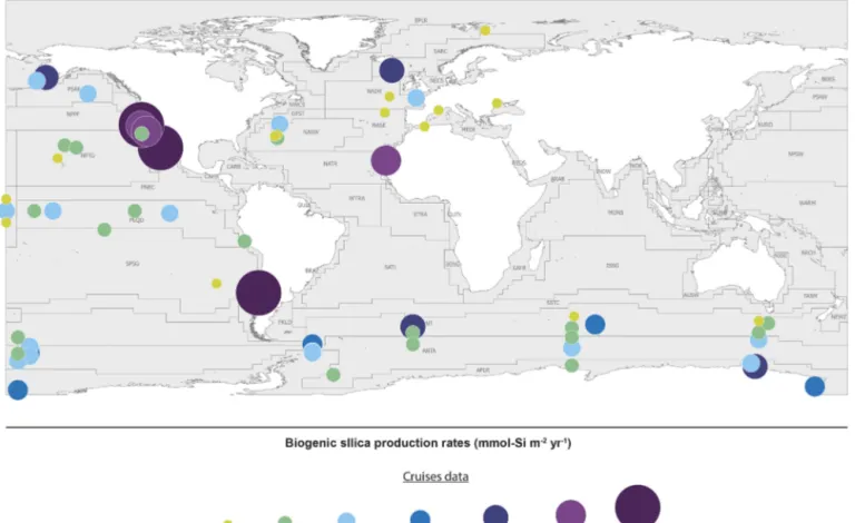
The last evaluation of global marine silica production was by Nelson et al. (1995), who estimated global gross marine bSi pelagic production to be 240(±40) Tmol Si yr−1. Since 1995, the number of field studies of bSi production (using either the30Si tracer method, Nelson and Goering (1977), or the 32Si method (Tréguer et al., 1991; Brzezinski and Phillips, 1997)) has grown substantially from 15 (1995) to 49 in 2019, allowing the first estimate based on empirical sil-ica production rate measurements (Fig. 3 and Sect. S4 in the Supplement). It is usually assumed that the silica production, as measured using the above methods, is mostly supported by diatoms, with some unknown (but minor) contribution of other planktonic species.
The silica production rates measured during 49 field cam-paigns were assigned to Longhurst provinces (Longhurst, 2007; Longhurst et al., 1995) based on location, with the ex-ception of the SO, where province boundaries were defined according to Tréguer and Jacques (1992). Extrapolating these “time-and-space-limited” measurements of bSi spatially to a biogeographic province, and annually from the bloom phe-nology for each province (calculated as the number of days where the chlorophyll concentration is greater than the aver-age concentration between the maximum and the minimum values), results in annual silica production estimates for 26 of the 56 world ocean provinces. The annual production of all provinces in a basin were averaged for the “ocean basin”
esti-Figure 3. Biogenic silica production measurements in the world ocean. Distribution of stations in the Longhurst biogeochemical provinces (Longhurst, 2007; Longhurst et al., 1995). All data are shown in Sect. S4 in the Supplement (Annex 1).
mate (Table 2) and then extrapolated by basin area. The aver-ages from provinces were subdivided among coastal for the “domain” estimate (Table 2), SO, and open-ocean domains and extrapolated based on the area of each domain. Averag-ing the ocean basin and the domain estimates (Table 2), our best estimate for the annual global marine bSi production is 267(±18) Tmol Si yr−1(Table 2).
4.1.2 Annual bSi pelagic production from models
Estimates of bSi production were also derived from satel-lite productivity models and from global ocean biogeo-chemical models (GOBMs). We used global net primary production (NPP) estimates from the carbon-based produc-tivity model (Westberry et al., 2008) and the vertically generalized productivity model (VGPM) (Behrenfeld and Falkowski, 1997) for the estimates based on satellite pro-ductivity models. NPP estimates from these models were divided into oligotrophic (< 0.1 µg chl a L−1), mesotrophic (0.1–1.0 µg chl a L−1), and eutrophic (> 1.0 µg chl a L−1) ar-eas (Carr et al., 2006). The fraction of productivity by di-atoms in each area was determined using the DARWIN model (Dutkiewicz et al., 2015), allowing a global
esti-mate where diatoms account for 29 % of the production. Each category was further subdivided into high-nutrient low-chlorophyll (HNLC) zones (> 5 µM surface nitrate; Garcia et al., 2014), coastal zones (< 300 km from a coastline), and open-ocean (remainder) zones for application of Si : C ratios to convert to diatom silica production. Si : C ratios were 0.52 for HNLC regions, 0.065 for the open ocean, and 0.13 for the coastal regions, reflecting the effect of Fe limitation in HNLC areas (Franck et al., 2000), of Si limitation for uptake in the open ocean (Brzezinski et al., 1998, 2011; Brzezinski and Nelson, 1996; Krause et al., 2012), and of replete con-ditions in the coastal zone (Brzezinski, 1985). Silica produc-tion estimates were then subdivided between coast (within 300 km of shore), open ocean, and SO (northern boundary 43◦S from Australia to South America, 34.8◦S from South
America to Australia) and summed to produce regional esti-mates (Table 2). Our best estimate for the global marine bSi production is 207(±23) Tmol Si yr−1 from satellite produc-tivity models (Table 2).
A second model-based estimate of silica production used 18 numerical GOBMs models of the marine silica cy-cle that all estimated global silica export from the surface ocean (Gnanadesikian and Toggweiler, 1999; Usbeck, 1999;
Table 1. Si inputs, outputs, and biological fluxes at word ocean scale.
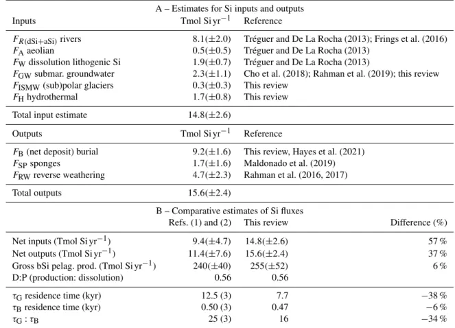
A – Estimates for Si inputs and outputs Inputs Tmol Si yr−1 Reference
FR(dSi+aSi)rivers 8.1(±2.0) Tréguer and De La Rocha (2013); Frings et al. (2016) FAaeolian 0.5(±0.5) Tréguer and De La Rocha (2013)
FWdissolution lithogenic Si 1.9(±0.7) Tréguer and De La Rocha (2013)
FGWsubmar. groundwater 2.3(±1.1) Cho et al. (2018); Rahman et al. (2019); this review FISMW(sub)polar glaciers 0.3(±0.3) This review
FHhydrothermal 1.7(±0.8) This review Total input estimate 14.8(±2.6)
Outputs Tmol Si yr−1 Reference
FB(net deposit) burial 9.2(±1.6) This review, Hayes et al. (2021) FSPsponges 1.7(±1.6) Maldonado et al. (2019) FRWreverse weathering 4.7(±2.3) Rahman et al. (2016, 2017) Total outputs 15.6(±2.4)
B – Comparative estimates of Si fluxes
Refs. (1) and (2) This review Difference (%) Net inputs (Tmol Si yr−1) 9.4(±4.7) 14.8(±2.6) 57 % Net outputs (Tmol Si yr−1) 11.4(±7.6) 15.6(±2.4) 37 % Gross bSi pelag. prod. (Tmol Si yr−1) 240(±40) 255(±52) 6 % D:P (production: dissolution) 0.56 0.56
τGresidence time (kyr) 12.5 (3) 7.7 −38 % τBresidence time (kyr) 0.50 (3) 0.47 −6 %
τG:τB 25 (3) 16 −34 %
References are (1) Nelson et al. (1995) and (2) Tréguer and De La Rocha (2013). (3) Recalculated from our updated dSi inventory value; see Supplement for detailed definition of flux term (in detailed legend of Fig. 1).
Table 2. Biological fluxes (FPgrossin Tmol Si yr−1).
World ocean Coast Southern Ocean Open ocean Silica production from models
– Satellite productivity models 207(±23) 56(±18) 60(±12) 91(±2) – Ocean biogeochemical models 276(±22) 129(±19)
Average of models 242(±49) Silica production field studies
– Ocean basin 249
– Domain 285 138 67 80
Average of field studies 267(±18) Global estimate 255(±52)
Global silica production as determined from numerical models and extrapolated from field measurements of silica production (uncertainties are standard errors).
Heinze et al., 2003; Wischmeyer et al., 2003; Jin et al., 2006; Dunne et al., 2007; Sarmiento et al., 2007; Bernard et al., 2011; Ward et al., 2012; Matsumoto et al., 2013; De Souza et al. 2014; Holzer et al., 2014; Aumont et al., 2015; Dutkiewicz et al., 2015; Pasquier and Holzer, 2017; Roshan et al., 2018). These include variants of the MOM,
HAMOCC OCIM, DARWIN, cGENIE, and PICES mod-els. Export production was converted to gross silica produc-tion by using a silica dissoluproduc-tion-to-producproduc-tion (D : P) ratio for the surface open ocean of 0.58 and 0.51 for the sur-face of coastal regions (Tréguer and De La Rocha, 2013). Model results were first averaged within variants of the same
model and then averaged across models to eliminate bi-assing the average to any particular model. Our best esti-mate from GOBMs for the global marine bSi production is 276(±23) Tmol Si yr−1 (Table 2). Averaging the estimates calculated from satellite productivity models and GOBMs gives a value of 242(±49) Tmol Si yr−1 for the global ma-rine bSi production (Table 2).
4.1.3 Best estimate for annual bSi pelagic production Using a simple average of the “field” and “model” es-timates, the revised best estimate of global marine gross bSi production, mostly due to diatoms, is now FPgross=
255(±52) Tmol Si yr−1, not significantly different from the Nelson et al. (1995) value.
In the SO, a key area for the world ocean Si cycle (De-Master, 1981), there is some disagreement among the dif-ferent methods of estimating bSi production. Field studies give an estimate of 67 Tmol Si yr−1 for the annual gross production of silica in the SO, close to the estimate of 60 Tmol Si yr−1calculated using satellite productivity mod-els (Table 2). However, the bSi production in the SO esti-mated by ocean biogeochemical models is about twice as high, at 129 Tmol Si yr−1(Table 2). The existing in situ bSi production estimates are too sparse to be able to definitively settle whether the lower estimate or the higher estimate is correct, but there is reason to believe that there are poten-tial biases in both the satellite NPP models and the ocean biogeochemical models. SO chlorophyll concentrations may be underestimated by as much as a factor of 3–4 (Johnson et al., 2013), which affects the NPP estimates in this region and hence our bSi production estimates with this method. The bSi production estimated by ocean biogeochemical mod-els is highly sensitive to vertical exchange rates in the SO (Gnanadesikan and Toggweiler, 1999) and is also dependent on the representation of phytoplankton classes in models with explicit representation of phytoplankton. Models that have excessive vertical exchange in the SO (Gnanadesikan and Toggweiler, 1999), or that represent all large phytoplank-ton as diatoms, may overestimate the Si uptake by plankphytoplank-ton in the SO. Other sources of uncertainty in our bSi production estimates include poorly constrained estimates of the Si : C ratio and dissolution-to-production ratios (see Sect. S4 in the Supplement). The errors incurred by these choices are more likely to cancel out in the global average but could be sig-nificant at regional scales, potentially contributing to the dis-crepancies in SO productivity across the various methods. 4.1.4 Estimates of the bSi production of other pelagic
organisms
Extrapolations from field and laboratory work show that the contribution of picocyanobacteria (like Synechococcus; Baines et al. 2012, Brzezinski et al., 2017; Krause et al., 2017) to the world ocean accumulation of bSi is <
20 Tmol Si yr−1. The gross silica production of rhizarians, siliceous protists, in the 0–1000 m layer might range between 2–58 Tmol Si yr−1, about 50 % of it occurring in the 0–200 m layer (Llopis Monferrer et al., 2020).
Note that these preliminary estimates of bSi accumulation or production by picocyanobacteria and rhizarians are within the uncertainty of our best estimate of FPgross.
4.2 Estimates of the bSi production of benthic organisms
The above-updated estimate of the pelagic production does not take into account bSi production by benthic organisms like benthic diatoms and sponges. Our knowledge of the pro-duction terms for benthic diatoms is poor, and no robust es-timate is available for bSi annual production of benthic di-atoms at a global scale (Sect. S4 in the Supplement).
Substantial progress has been made for silica deposition by siliceous sponges recently. Laboratory and field studies reveal that sponges are highly inefficient in the molecular transport of dSi compared to diatoms and consequently bSi production, particularly when dSi concentrations are lower than 75 µM, a situation that applies to most ocean areas (Mal-donado et al., 2020). On average, sponge communities are known to produce bSi at rates that are about 2 orders of magnitude smaller than those measured for diatom commu-nities (Maldonado et al., 2012). The global standing crop of sponges is very difficult to be constrained. The annual bSi production attained by such standing crop is even more diffi-cult to estimate because sponge populations are not homo-geneously distributed on the marine benthic environment, and extensive, poorly mapped, and unquantified aggrega-tions of heavily silicified sponges occur in the deep sea of all oceans. A first tentative estimate of bSi production for sponges on continental shelves, where sponge biomass can be more easily approximated, ranged widely, from 0.87 to 7.39 Tmol Si yr−1, because of persisting uncertainties in es-timating sponge standing crop (Maldonado et al., 2012). A way to estimate the global annual bSi production by sponges without knowing their standing crop is to retrace bSi pro-duction values from the amount of sponge bSi that is an-nually being deposited to the ocean bottom, after assuming that, in the long run, the standing crop of sponges in the ocean is in equilibrium (i.e it is neither progressively increas-ing nor decreasincreas-ing over time). The deposition rate of sponge bSi has been estimated at 49.95(±74.14) mmol−Si m−2yr−1 on continental margins, at 0.44(±0.37) mmol − Si m−2yr−1 in sediments of ocean basins where sponge aggregations do not occur, and at 127.30(±105.69) mmol − Si m−2yr−1 in deep-water sponge aggregations (Maldonado et al., 2019). A corrected sponge bSi deposition rate for ocean basins is estimated at 2.98(±1.86) mmol − Si m−2yr−1 assuming that sponge aggregations do not occupy more than 2 % of seafloor of ocean basins (Maldonado et al., 2019). A total value of 6.15(±5.86) Tmol Si yr−1 can be estimated
for the global ocean when the average sponge bSi depo-sition rate for continental margins and seamounts (repre-senting 108.02 million squarekilometers of seafloor) and for ocean basins (253.86 million squarekilometers) is scaled up through the extension of those bottom compartments. If the bSi production being accumulated as standing stock in the living sponge populations annually is assumed to become constant in a long-term equilibrium state, the global annual deposition rate of sponge bSi can be considered a reliable estimate of the minimum value that the annual bSi produc-tion by the sponges can reach in the global ocean. The large associated SD value does not derive from the approach be-ing unreliable but from the spatial distribution of the sponges on the marine bottom being extremely heterogeneous, with some ocean areas being very rich in sponges and sponge bSi in sediments at different spatial scales while other areas are completely deprived of these organisms.
5 Discussion
5.1 Overall residence times
The overall geological residence time for Si in the ocean (τG) is equal to the total amount of dSi in the ocean
di-vided by the net input (or output) flux. We re-estimate the total ocean dSi inventory value derived from the Pandora model (Peng et al. 1993), which according to Tréguer et al. (1995) was 97 000 Tmol Si. An updated estimate of the global marine dSi inventory was computed by interpolating the objectively analyzed annual mean silicate concentrations from the 2018 World Ocean Atlas (Garcia et al., 2019) to the OCIM model grid (Roshan et al., 2018). Our estimate is now 120 000 Tmol Si, i.e., about 24 % higher than the Tréguer et al. (1995) estimate. Tables 1B and 3 show updated esti-mates of τG from Tréguer et al. (1995) and Tréguer and De
La Rocha (2013) using this updated estimate of the total dSi inventory. Our updated budget (Fig. 1, Tables 1B and 3A) re-duces past estimates of τG(Tréguer et al., 1995; Tréguer and
De La Rocha, 2013) by more than half, from ca. 18 kyr to ca. 8 kyr (Table 3C). This brings the ocean residence time of Si closer to that of nitrogen (< 3 kyr; Sarmiento and Gruber, 2006) than phosphorus (30–50 kyr; Sarmiento and Gruber, 2006).
The overall biological residence time, τB, is calculated by
dividing the total dSi content of the world ocean by gross sil-ica production. It is calculated from the bSi pelagic produc-tion only given the large uncertainty on our estimate of the bSi production by sponges. τBis ca. 470 years (Tables 1B
and 3). Thus, Si delivered to the ocean passes through the biological uptake and dissolution cycle on average 16 times (τG/τB)before being removed to the sea floor (Tables 1B and
3C).
The new estimate for the global average preservation efficiency of bSi buried in sediments is (FB/FPgross=
(9.2/255) =) 3.6 %, which is similar to the Tréguer and De La Rocha (2013) estimate. This makes bSi in sediments an intriguing potential proxy for export production (Tréguer et al., 2018). Note that the reverse weathering flux (FRW) is
also fed by the export flux (FE) (Fig. 4). So, the
preserva-tion ratio of biogenic silica in sediment can be calculated as (FB+FRW)/FPgross=(13.9/255) = 5.45 %, which is ≈ 30
times larger than the carbon preservation efficiency. 5.2 The issue of steady state
Over a given timescale, an elemental cycle is at steady state if the outputs balance the inputs in the ocean and the mean concentration of the dissolved element remains constant. 5.2.1 Long timescales (> τG)
Over geologic timescales, the average dSi concentration of the ocean has undergone drastic changes. A seminal work (Siever, 1991) on the biological–geochemical interplay of the Si cycle showed a decline of a factor of 100 in ocean dSi con-centration from 550 Myr ago to the present. This decline was marked by the rise of silicifiers like radiolarian and sponges during the Phanerozoic. Then during the mid-Cenozoic di-atoms started to dominate a Si cycle previously controlled by inorganic and diagenetic processes. Conley et al. (2017) hypothesized that biological processes might also have in-fluenced the dSi concentration of the ocean at the start of oxygenic photosynthesis, taking into account the impact of the evolution of biosilicifying organisms (including bacteria-related metabolism). There is further evidence that the exist-ing lineages of sponges have their origin in ancient (Meso-zoic) oceans with much higher dSi concentrations than the modern ocean. Some recent sponge species can only com-plete their silica skeletons if dSi concentration much higher than that in their natural habitat is provided experimentally (Maldonado et al., 1999). Also, all recent sponge species in-vestigated to date have kinetics of dSi consumption that reach their maximum speed only at dSi concentrations that are 1 to 2 orders of magnitude higher than the current dSi availability in the sponge habitats, indicating that the sponge physiology evolved in dSi-richer ancestral scenarios. Note that with a ge-ological residence time of Si of ca. 8000 years, the Si cycle can fluctuate over glacial–interglacial timescales.
5.2.2 Short timescales (< τG)
In the modern ocean the main control over silica burial and authigenic formation rate is the bSi production rate of pelagic and benthic silicifiers, as shown above. The gross produc-tion of bSi due to diatoms depends on the dSi availability in the surface layer (Fig. 1). Silicic acid does not appear to be limiting in several zones of the world ocean, which in-clude the coastal zones and the HNLC zones (Tréguer and De La Rocha, 2013). Note that any short-term change of dSi inputs does not imply modification of bSi production, or
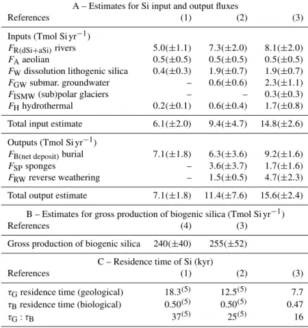
ex-Table 3. A total of 25 years of evolution of the estimates for Si inputs, outputs, biological production, and residence times at World Ocean scale.
A – Estimates for Si input and output fluxes
References (1) (2) (3)
Inputs (Tmol Si yr−1)
FR(dSi+aSi)rivers 5.0(±1.1) 7.3(±2.0) 8.1(±2.0) FAaeolian 0.5(±0.5) 0.5(±0.5) 0.5(±0.5) FWdissolution lithogenic silica 0.4(±0.3) 1.9(±0.7) 1.9(±0.7) FGWsubmar. groundwater – 0.6(±0.6) 2.3(±1.1) FISMW(sub)polar glaciers – – 0.3(±0.3) FHhydrothermal 0.2(±0.1) 0.6(±0.4) 1.7(±0.8) Total input estimate 6.1(±2.0) 9.4(±4.7) 14.8(±2.6) Outputs (Tmol Si yr−1)
FB(net deposit)burial 7.1(±1.8) 6.3(±3.6) 9.2(±1.6) FSPsponges – 3.6(±3.7) 1.7(±1.6) FRWreverse weathering – 1.5(±0.5) 4.7(±2.3) Total output estimate 7.1(±1.8) 11.4(±7.6) 15.6(±2.4)
B – Estimates for gross production of biogenic silica (Tmol Si yr−1)
References (4) (3)
Gross production of biogenic silica 240(±40) 255(±52) C – Residence time of Si (kyr)
References (1) (2) (3)
τGresidence time (geological) 18.3(5) 12.5(5) 7.7 τBresidence time (biological) 0.50(5) 0.50(5) 0.47 τG:τB 37(5) 25(5) 16
References are as follows. (1) Tréguer et al. (1995). (2) Tréguer and De La Rocha (2013). (3) This review. (4) Nelson et al. (1995).(5)Recalculated from our updated dSi inventory value.
port or burial rate. For this reason, climatic changes or an-thropogenic impacts that affect dSi inputs to the ocean by rivers and/or other pathways could lead to an imbalance of Si inputs and outputs in the modern ocean.
5.2.3 A possible steady-state scenario
Within the limits of uncertainty, the total net inputs of dSi and aSi are 14.8(±2.6) Tmol Si yr−1 and are approx-imately balanced by the total net output flux of Si of 15.6(±2.4) Tmol Si yr−1. Figure 1 supports the hypothesis that the modern ocean Si cycle is at steady state, compatible with the geochemical and biological fluxes of Table 1.
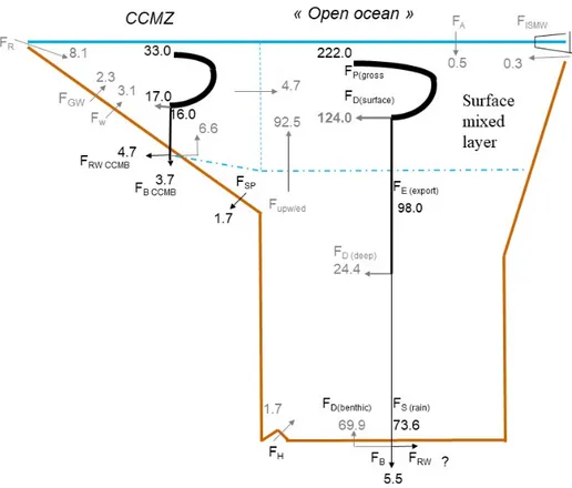
Consistent with Fig. 1, Fig. 4 shows a steady-state scenario for the Si cycle in the coastal and continental margin zone (CCMZ), often called the “boundary exchange” zone which, according to Jeandel (2016) and Jeandel and Oelkers (2015), plays a major role in the land-to-ocean transfer of material (also see Fig. 2). Figure 4 illustrates the interconnection be-tween geochemical and biological Si fluxes, particularly in the CCMZ. In agreement with Laruelle et al. (2009), Fig. 4 also shows that the open-ocean bSi production is mostly
fu-eled by dSi inputs from below (92.5 Tmol Si yr−1) and not by the CCMZ (4.7 Tmol Si yr−1) (Sect. S5 in the Supplement). 5.3 The impacts of global change on the Si cycle As illustrated by Figs. 1 and 4, the pelagic bSi production is mostly fueled from the large recycled deep-ocean pool of dSi. This lengthens the response time of the Si cycle to changes in dSi inputs to the ocean due to global change (in-cluding climatic and anthropogenic effects), increasing the possibility for the Si cycle to be out of balance.
5.3.1 Impacts on riverine inputs of dSi and aSi
Climate change at short timescales during the 21st century impacts the ocean delivery of riverine inputs of dSi and aSi (FR) and of the terrestrial component of the
subma-rine groundwater discharge (FGW), either directly (e.g., dSi
and aSi weathering and transport) or indirectly by affecting forestry and agricultural dSi export. So far the impacts of cli-mate change on the terrestrial Si cycle have been reported for boreal wetlands (Struyf et al., 2010), North American (Opalinka and Cowling, 2015) and western Canadian
Arc-Figure 4. Schematic view of the Si cycle in the coastal and continental margin zone (CCMZ), linked to the rest of the world ocean (open-ocean zone, including upwelling and polar zones). In this steady-state scenario, consistent with Fig. 1, total inputs = total outputs = 15.6 Tmol Si yr−1. This figure illustrates the links between biological, burial, and reverse weathering fluxes. It also shows that the open-ocean bSi (pelagic) production (FP(gross)=222 Tmol Si yr−1) is mostly fueled by dSi inputs from below 92.5 Tmol Si yr−1, with the CCMZ only providing 4.7 Tmol Si yr−1to the open ocean.
tic rivers (Phillips, 2020), and the tributaries of the Laptev and East Siberian seas (Charette et al., 2020), but not for tropical environments. Tropical watersheds are the key ar-eas for the transfer of terrestrial dSi to the ocean, as approx-imately 74 % of the riverine Si input is from these regions (Tréguer et al., 1995). Precipitation in tropical regions usu-ally follows the “rich-get-richer” mechanism in a warming climate according to model predictions (Chou et al., 2004, 2008). In other words, in tropical convergence zones rainfall increases with climatological precipitation, but the opposite is true in tropical subsidence regions, creating diverging im-pacts for the weathering of tropical soils. If predictions of global temperature increase and variations in precipitations of the IPCC are correct (IPCC, 2018), it is uncertain how FR
or FGW, two major components of dSi and aSi inputs, will
change. Consistent with these considerations are the conclu-sions of Phillips (2020) on the impacts of climate change on the riverine delivery of dSi to the ocean, using a machine-learning-based approach. Phillips (2020) predicts that within the end of this century dSi mean yield could increase region-ally (for instance in the Arctic region), but the global mean dSi yield is projected to decrease, using a model based on
30 environmental variables including temperature, precipita-tion, land cover, lithology, and terrain.
5.3.2 Abundance of marine and pelagic and benthic silicifiers
A change in diatom abundance was not seen on the North Atlantic from continuous plankton recorder (CPR) data over the period 1960–2009 (Hinder et al., 2012). However, stud-ies have cautioned that many fields (e.g., chl) will take sev-eral decades before these changes can be measured precisely beyond natural variability (Henson et al 2010; Dutkiewicz et al 2019). The melting of Antarctic ice platforms has al-ready been noticed to trigger impressive population blooms of highly silicified sponges (Fillinger et al., 2013).
5.3.3 Predictions for the ocean phytoplankton production and bSi production
Climate change in the 21st century will affect ocean circula-tion, stratificacircula-tion, and upwelling and therefore nutrient cy-cling (Aumont et al., 2003; Bopp et al., 2005, 2013). With increased stratification, dSi supply from upwelling will de-crease (Figs. 1 and 4), leading to less siliceous phytoplankton
production in surface compartments of lower latitudes and possibly the North Atlantic (Tréguer et al., 2018). The im-pact of climate change on the phytoplankton production in polar seas is highly debated as melting of sea ice decreases light limitation. In the Arctic Ocean an increase in nutrient supply from river- and shelf-derived waters (at the least for silicic acid) will occur through the Transpolar Drift, poten-tially impacting rates of primary production, including bSi production (e.g., Charette et al., 2020). In the SO bSi produc-tion may increase in the coastal and continental shelf zone as iron availability increases due to ice sheet melt and ice-berg delivery (Duprat et al., 2016; Boyd et al., 2016; Herraiz-Borreguero et al., 2016; Hutchins and Boyd, 2016; Tréguer et al., 2018; Hawkings et al., in press). However, Henley et al. (2019) suggest a shift from diatoms to haptophytes and cryp-tophytes with changes in ice coverage in the western Antarc-tic Peninsula. How such changes in coastal environments and nutrient supplies will interplay is unknown. Globally, it is very likely that a warmer and more acidic ocean alters the pelagic bSi production rates, thus modifying the export pro-duction and outputs of Si at short timescales.
Although uncertainty is substantial, modeling studies (Bopp et al., 2005; Laufkötter et al., 2015; Dutkiewicz et al., 2019) suggest regional shifts in bSi pelagic production with climatic change. These models predict a global decrease in diatom biomass and productivity over the 21st century (Bopp et al., 2005, Laufkötter et al., 2015; Dutkiewicz et al., 2019), which would lead to a reduction in the pelagic biological flux of silica. Regional responses differ, with most models sug-gesting a decrease in diatom productivity in the lower lati-tudes and many predicting an increase in diatom productiv-ity in the SO (Laufkötter et al., 2015). Holzer et al. (2014) suggest that changes in supply of dissolved iron (dFe) will alter bSi production mainly by inducing floristic shifts, not by relieving kinetic limitation. Increased primary productiv-ity is predicted to come from a reduction in sea ice area, faster growth rates in warmer waters, and longer growing seasons in the high latitudes. However, many models have very simple ecosystems including only diatoms and small phytoplankton. In these models, increased primary produc-tion in the SO is mostly from diatoms. Models with more complex ecosystem representations (i.e., including additional phytoplankton groups) suggest that increased primary pro-ductivity in the future SO will be due to other phytoplank-ton types (e.g., pico-eukaryote) and that diatoms’ biomass will decrease (Dutkiewicz et al., 2019; also see model Plank-TOM5.3 in Laufkötter et al., 2015), except in regions where sea ice cover has decreased. Differences in the complexity of the ecosystem and parameterizations, in particular in terms of temperature dependences of biological process, between models lead to widely varying predictions (Laufkotter et al., 2015; Dutkiewicz et al., 2019). These uncertainties suggest we should be cautious in our predictions of what will happen with the silica biogeochemical cycle in a future ocean.
5.4 Other anthropogenic impacts
For decades if not centuries, anthropogenic activities directly or indirectly altered the Si cycle in rivers and the CCMZ (Conley et al., 1993; Ittekot et al., 2000, 2006; Derry et al., 2005; Humborg et al., 2006; Laruelle et al., 2009; Bernard et al., 2010; Liu et al., 2012; Yang et al., 2015; Wang et al., 2018a; Zhang et al., 2019). Processes involved include eu-trophication and pollution (Conley et al., 1993; Liu et al., 2012), river damming (Ittekot et al., 2000; Ittekot et al., 2006; Yang et al., 2015; Wang et al., 2018), deforestation (Conley et al., 2008), changes in weathering and in river discharge (Bernard et al., 2010; Yang et al., 2015), and deposition load in river deltas (Yang et al., 2015).
Among these processes, river damming is known for hav-ing the most spectacular and short-timescale impacts on the Si delivery to the ocean. River damming favors enhanced biologically mediated absorption of dSi in the dam reser-voir, thus resulting in significant decreases in dSi concen-tration downstream. Drastic perturbations in the Si cycle and downstream ecosystem have been shown (Ittekot et al., 2000; Humborg et al., 2006; Ittekot, 2006; Zhang et al., 2019), par-ticularly downstream of the Nile (Mediterranean Sea), the Danube (Black Sea), and the fluvial system of the Baltic Sea. Damming is a critical issue for major rivers of the tropi-cal zone (Amazon, Congo, Changjiang, Huanghe, Ganges, Brahmaputra, etc.), which carry 74 % of the global exorheic dSi flux (Tréguer et al., 1995; Dürr et al., 2011). Among these major rivers, the course of the Amazon and Congo is, so far, not affected by a dam or, as for the Congo River, the con-sequence of Congo damming for the Si cycle in the equato-rial African coastal system has not been studied. The case of Changjiang (Yangtze), one of the major world players in dSi delivery to the ocean, is of particular interest. Interestingly, the Changjiang (Yangtze) River dSi concentrations decreased dramatically from the 1960s to 2000 (before the building of the Three Gorges Dam, TGD). This decrease is attributed to a combination of natural and anthropogenic impacts (Wang et al., 2018a). Paradoxically, since the construction of the TGD (2006–2009) no evidence of additional retention of dSi by the dam has been demonstrated (Wang et al., 2018a).
Over the 21st century, the influence of climate change, and other anthropogenic modifications, will have variable im-pacts on the regional and global biogeochemical cycling of Si. The input of dSi will likely increase in specific regions (e.g., Arctic Ocean), whilst inputs to the global ocean might decrease. Global warming will increase stratification of the surface ocean, leading to a decrease in dSi inputs from the deep sea, although this is unlikely to influence the Southern Ocean (see Sect. 5.3.3). Model-based predictions suggest a global decrease in diatom production, with a subsequent de-crease in export production and Si burial rate. Clearly, new observations are needed to validate model predictions.
6 Conclusions and recommendations
The main question that still needs to be addressed is whether the contemporary marine Si cycle is at steady state, which requires the uncertainty in total inputs and outputs to be min-imized.
For the input fluxes, more effort is required to quan-tify groundwater input fluxes, particularly using geochem-ical techniques to identify the recycled marine flux from other processes that generate a net input of dSi to the ocean. In light of laboratory experiments by Fabre et al. (2019) demonstrating low-temperature dissolution of quartz in clas-tic sand beaches, collective multinational effort should ex-amine whether sandy beaches are major global dSi sources to the ocean. Studies addressing uncertainties at the regional scale are critically needed. Further, better constraints on hy-drothermal inputs (for the northeast Pacific-specific case), ae-olian input, and subsequent dissolution of minerals both in the coastal and in open-ocean zones and inputs from ice melt in polar regions are required.
For the output fluxes, it is clear that the alkaline digestion of biogenic silica (DeMaster, 1981; Mortlock and Froelich, 1989, Müller and Schneider, 1993), one of the commonly used methods for bSi determination in sediments, is not al-ways effective at digesting all the bSi present in sediments. This is especially true for highly silicified diatom frustules, radiolarian tests, or sponge spicules (Maldonado et al., 2019; Pickering et al., 2020). Quantitative determination of bSi is particularly difficult for lithogenic or silicate-rich sediments (e.g., estuarine and coastal zones), for example those of the Chinese seas. An analytical effort for the quantitative deter-mination of bSi from a variety of sediment sources and the organization of an international comparative analytical exer-cise are of high priority for future research. It is also clear that reverse weathering processes are important not only in estuarine or coastal environments, but also in distal coastal zones, slope, and open-ocean regions of the global ocean (Michalopoulos and Aller, 2014; Chong et al., 2016; Ehlert et al., 2016a; Baronas et al., 2017; Geilert et al., 2020; Picker-ing et al., 2020). Careful use of geochemical tools (e.g.,32Si, Ge/Si, δ30Si: Ehlert et al., 2016; Ng et al., 2020; Geilert et al., 2020; Pickering et al., 2020; Cassarino et al., in press) to trace partitioning of bSi between opal and authigenic clay phases may further elucidate the magnitude of this sink, par-ticularly in understudied areas of the ocean.
This review highlights the significant progress that has been made in the past decade toward improving our quan-titative and qualitative understanding of the sources, sinks, and internal fluxes of the marine Si cycle. Filling the knowl-edge gaps identified in this review is also essential if we are to anticipate changes in the Si cycle, and their ecological and biogeochemical impacts, in the future ocean.
Data availability. All data used in this review article are available in the referenced articles. Data of biogenic pelagic production are shown in the Supplement (Annex 1).
Supplement. The supplement related to this article is available on-line at: https://doi.org/10.5194/bg-18-1269-2021-supplement.
Author contributions. PJT and JNS defined the manuscript content and wrote the paper. MAC, CE, JH, SR, OR, and PT wrote the input section. JS, CE, SR, and MM wrote the output section. MB, TD, SD, AL, and PT wrote the pelagic production section. MLA and MM wrote the sponge subsections. SML, LR, and PT wrote the discussion section. Every author re-read and approved the review article.
Competing interests. The authors declare that they have no conflict of interest.
Acknowledgements. The idea for this paper was conceived during a conference of the SILICAMICS Network, held in June 2018 at the University of Victoria (Canada). Thanks are due to Sébastien Hervé (LEMAR-IUEM, Plouzané) for his artwork.
Financial support. This work was supported by the French Na-tional Research Agency (18-CEO1-0011-01) and by the Span-ish Ministry of Science, Innovation and Universities (PID2019-108627RB-I00).
Review statement. This paper was edited by Emilio Marañón and reviewed by two anonymous referees.
References
Aller, R. C.: Sedimentary diagenesis, depositional environments, and benthic fluxes, in: Treatise on Geochemistry: Second edition, edited by: Holland, H. D. and Turekian, K. K., Elsevier, Oxford, 8, 293–334, 2014.
Aller, R. C., Blair, N. E., and Brunskill, G. J.: Early diagenetic cy-cling, incineration, and burial of sedimentary organic carbon in the central Gulf of Papua (Papua New Guinea), J. Geophys. Res. Earth Surf., 113, 1–22, 2008.
Aller, R. C., Blair, N. E., Xia, Q., and Rude, P. D.: Remineraliza-tion rates, recycling, and storage of carbon in Amazon shelf sed-iments, Cont. Shelf Res., 16, 753–786, 1996.
Anschutz, P., Smith, T., Mouret, A., Deborde, J., Bujan, S., Poirier, D., and Lecroart, P.: Tidal sands as biogeochemical reactors, Es-tuar. Coast. Shelf Sci., 84, 84–90, 2009.
Arsouze, T., Dutay, J.-C., Lacan, F., and Jeandel, C.: Recon-structing the Nd oceanic cycle using a coupled dynami-cal – biogeochemidynami-cal model, Biogeosciences, 6, 2829–2846, https://doi.org/10.5194/bg-6-2829-2009, 2009.