Levenberg-Marquardt Algorithm for Zero and Non-zero Residual Inverse Problems

Convergence and Iteration Complexity Analysis of a

Levenberg-Marquardt Algorithm for Zero and Non-zero Residual Inverse Problems

E. Bergou

^∗

Y. Diouane

^†

V. Kungurtsev

^‡

January 28, 2018

Abstract

The Levenberg-Marquardt algorithm is one of the most popular algorithms for the solu- tion of nonlinear least squares problems. In this paper, we propose and analyze the global and local convergence results of a novel Levenberg-Marquardt method for solving general nonlinear least squares problems. The proposed algorithm enjoys strong convergence prop- erties (global convergence as well as local convergence) for least squares problems which do not necessarily have a zero residual solution, all without any additional globalization strategy.

Furthermore, we proved worst-case iteration complexity bounds for the proposed algorithm.

Preliminary numerical experiments confirm the theoretical behavior of our proposed algo- rithm.

Keywords: Nonlinear least squares problem, inverse problems, Levenberg-Marquardt method, global and local convergence, worst-case complexity bound, quadratic and linear convergence.

1 Introduction

In this paper we consider the general nonlinear least squares problem

x∈

min

Rⁿ

f (x) = 1

2 kF (x)k

²

, (1)

where F : R

ⁿ

→ R

^m

is a (deterministic) vector-valued function, assumed continuously differ- entiable.We do not assume that there is a solution with zero residual, or that we seek such a solution. In fact, problems of this nature arise in several important practical contexts. One example is inverse problems [16] (e.g., data assimilation [4, 17], full-waveform inversion [20]), where typically an ill-posed nonlinear continuous problem is solved through a discretization.

Other examples appear in parameter estimation when a mathematical model approximating a true distribution is fit to given (noisy) data [16, 20]. In all these cases, the resulting least squares problems do not necessarily have a zero residual at any point but may be small.

∗MaIAGE, INRA, Universit´e Paris-Saclay, 78350 Jouy-en-Josas, France ([email protected]).

†Institut Sup´erieur de l’A´eronautique et de l’Espace (ISAE-SUPAERO), Universit´e de Toulouse, 31055 Toulouse Cedex 4, France ([email protected]).

‡Department of Computer Science, Faculty of Electrical Engineering, Czech Technical University in Prague. Support for this author was provided by the Czech Science Foundation project 17-26999S ([email protected]).

Recall that the Gauss-Newton method is an iterative procedure for solving (1) and where at each iterate x

j

a step is computed as a solution to the linearized least squares subproblem

s∈

min

Rⁿ

1

2 kF

_j

+ J

_j

sk

²

,

where F

j

= F (x

j

) and J

j

= J (x

j

) denotes the Jacobian of F at x

j

. The subproblem has a unique solution if J

j

has full column rank, and in that case the step is a descent direction for f . The Levenberg-Marquardt method [11, 12] (see also [15]) was developed to deal with the rank deficiency of J

j

and to provide a globalization strategy for Gauss-Newton. At each iteration a step is considered of the form −(J

_j^>

J

j

+ γ

j

I)

⁻¹

J

_j^>

F

j

, corresponding to the unique solution of

s∈

min

Rⁿ

m

_j

(s) = 1

2 kF

_j

+ J

_j

sk

²

+ 1

2 γ

_j

ksk

²

, (2)

where γ

_j

> 0 is an appropriately chosen regularization parameter.

In this paper, we will present and analyze the global and local convergence results of a novel Levenberg-Marquardt method for solving general nonlinear least squares problems. In particular we present a Levenberg-Marquardt updating strategy that carefully balances the opposing objectives of ensuring global convergence and stabilizing a Newton local convergence regime.

The strongest results for local convergence of Levenberg-Marquardt are given in a series of papers beginning with [21] (such as [8] and [5], see also [6]), wherein it is assumed that the solution satisfies F (x) = 0. The algorithm we present matches this rate for zero-residual problems. In the case of non-zero residuals, it has been found that the implementations of Levenberg-Marquardt converge locally at a linear rate if the norm of the residual is sufficiently small and the parameter γ

j

goes to zero [10]. Our proof of linear convergence is simpler than in [10] as well as more completely complementing the other convergence results. Furthermore [10]

only show superlinear convergence for zero-residual problems and only present global convergence for exact solutions of subproblems. They also present additional analysis in regards for finite arithmetic that is different in scope of our work, however.

It should be noted that in general the goals of encouraging global and local convergence compete against each other. Namely, the regularization parameter appearing in the subproblem should be allowed to become arbitrarily large in order to encourage global convergence, to ensure the local accuracy of the linearized subproblem, but the parameter must approach zero in order to function as a stabilizing regularization that encourages fast local convergence.

For example, in the original presentation of the Levenberg-Marquardt method in [11, 12], γ

j

is not permitted to go to zero, and only global convergence is considered. By contrast, in [21], for instance, there is a two-phase method where quadratic decline in the residual is tested with each step that is otherwise globalized by a line-search procedure. Two phase methods, while also less mathematically elegant, are practically inefficient and challenging to implement in the sense that it can be difficult to properly ascertain when the region of local convergence is reached.

Our parameter updating strategy is inspired by [7], which presents a Levenberg-Marquardt method inspired from trust-region algorithm for zero residual least squares problems. The trust- region radius is updated as ∆

_j+1

= µkF

_j+1

k

^δ

, with δ ∈ (1/2; 1) and µ is updated according to classical global convergence updating strategies, the residual F

j+1

is included to enforce local convergence. They show global and superlinear local convergence properties for their method.

We extend the results outlined above in scope in the sense of showing the convergence properties

for residual problems which do not necessarily have a zero residual solution, as well as in elegance

in that the method is purely a Levenberg-Marquardt method, with no additional globalization

strategies, and thus is seamless and is an extension of the standard classical approach to least- squares problems, as well as improve the convergence rate to quadratic.

Furthermore, we establish a worst-case complexity analysis of our proposed algorithm. In fact, given a tolerance ∈ (0, 1), we aim at estimating the number of iterations needed to reach an iterate x

j

such that

k∇f (x

_j

)k < . (3)

Worst-case iteration complexity bounds of Levenberg-Marquardt methods applied to non-linear least squares problems using specific schemes of update for γ

_j

can be found in [18, 19, 22].

Up to a logarithmic factor, we show that our proposed algorithm has a complexity bounds that matches results previously cited Levenberg-Marquardt algorithms. Precisely, we obtain an iteration complexity bound in ˜ O

⁻²

, where the notation ˜ O(·) indicates the presence of logarithmic factors in . The logarithmic factor in our complexity analysis is due to our strategy of updating γ

_j

to ensure both global convergence and fast local convergence. We note that in [18, 19, 22] only the global convergence is shown.

1.1 Summary of Contributions

Our contribution amounts to the following. Whereas with the state of the art, in choosing a Levenberg-Marquardt method, one has four choices with regards to convergence and complexity guarantees, in particular

1. global convergence with the exact subproblem solution and a quadratic local convergence for zero-residual problems, or

2. global convergence with the exact and inexact subproblem solution for any (zero or nonzero residual) inverse problem, or,

3. global convergence and iteration complexity results for any inverse problem, or

4. global convergence, linear local convergence for non-zero residual problems, and superlinear convergence for zero-residual problems.

In this paper, we present a seamless (i.e., no separate phases) Levenberg-Marquardt method that simultaneously achieves,

1. global convergence for exact and inexact subproblem solutions for any inverse problem 2. iteration complexity results for any inverse problem,

3. linear local convergence rate for non-zero residual inverse problems, 4. quadratic local convergence rate for zero-residual inverse problems,

and thus match all of the best state of the art results in the literature with just one algorithm.

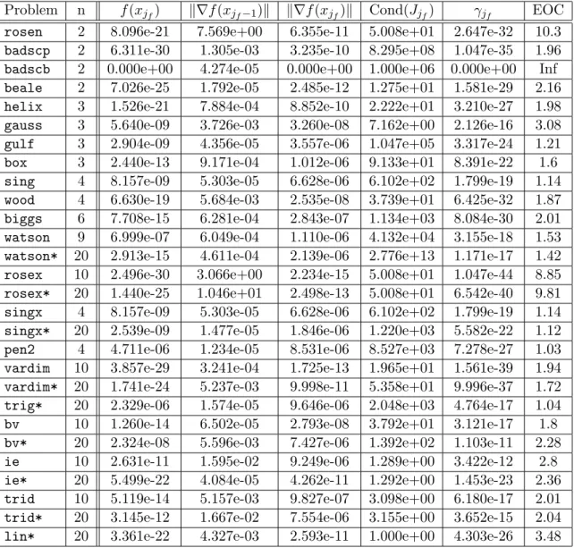
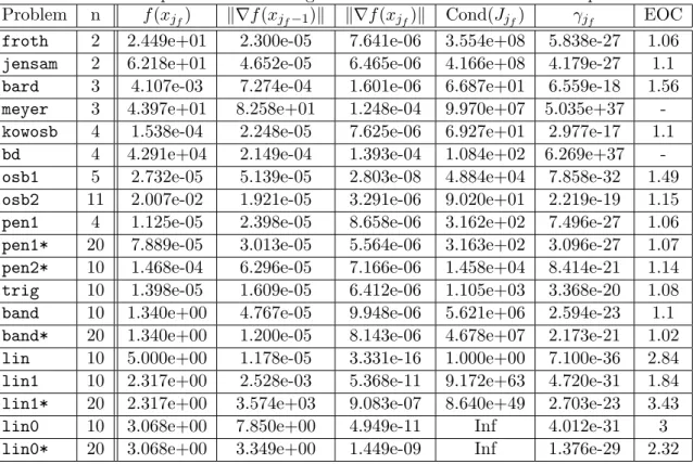
This is with a relatively simple procedure and standard proof techniques. In addition we present

a thorough set of numerical results demonstrating the order of convergence as well as the global

convergence properties of the method.

1.2 Outline and Notation

The outline of this paper is as follows. In Section 2 we present the proposed Levenberg- Marquardt algorithm for solving general nonlinear least squares problems. Section 3 addresses the inexact solution of the linearized least squares subproblems arising within the Levenberg- Marquardt method. In Section 4, we show the global convergence of our algorithm. Section 5 describes a worst-case complexity analysis of the proposed method. In Section 6 we derive the overall local convergence analysis of the proposed algorithm. In Section 7, preliminary numerical experiments with basic implementations are presented that show the good behavior of our novel algorithm. Finally, in Section 8 we draw some perspectives and conclusions.

Throughout this paper k · k will denote the vector or matrix l

2

-norm.

2 A novel Levenberg-Marquardt algorithm

In deciding whether to accept a step s

_j

generated by the subproblem (2), the Levenberg- Marquardt method can be seen as precursor of the trust-region method [3]. In fact, it seeks to determine when the Gauss-Newton step is applicable (in which case the regularization param- eter is set to zero) or when it should be replaced by a slower but safer steepest descent step (corresponding to a sufficiently large regularization parameter). For that purpose, one considers the ratio between the actual reduction f (x

j

) − f (x

j

+ s

j

) attained in the objective function and the reduction m

_j

(0) − m

_j

(s

_j

) predicted by the model, given by

ρ

j

= f(x

j

) − f (x

j

+ s

j

) m

_j

(0) − m

_j

(s

_j

) .

Then, if ρ

j

is sufficiently above zero, the step is accepted and γ

j

is possibly decreased. Otherwise the step is rejected and γ

_j

is increased.

In this paper we consider the choice of the regularization parameter as γ

_j

= µk∇f (x

_j

)k

²

. where µ is updated according to the ratio ρ

j

. The considered Levenberg-Marquardt algorithm is described below.

Algorithm 1: Levenberg-Marquardt algorithm.

Initialization

Choose the constants η ∈ (0, 1), µ

min

> 0 and λ > 1. Select x

0

and µ

0

≥ µ

min

. Set γ

0

= µ

0

k∇f(x

₀

)k

²

and ¯ µ = µ

0

.

For j = 0, 1, 2, . . .

1. Solve (or approximately solve) (2), and let s

j

denote such a solution.

2. Compute ρ

j

=

^f_m^{(xj)−f(xj+sj)}

j(0)−m_j(sj)

.

3. If ρ

j

≥ η, then set x

j+1

= x

j

+ s

j

and µ

j+1

∈ [max(µ

min

, µ/λ), ¯ µ] and ¯ ¯ µ = µ

j+1

. Otherwise, set x

_j+1

= x

_j

and µ

_j+1

= λµ

_j

.

4. Compute γ

j+1

= µ

j+1

k∇f (x

j+1

)k

²

.

A brief remark is warranted regarding the new step acceptance criteria. Note that we have

an auxiliary parameter ¯ µ, that represents the last good parameter. This is necessary in order to

balance the requirements of global and local convergence. If the model is relatively inaccurate, then µ

j

is driven higher, however, when we reach a region of local convergence, we need the parameter γ

_j

to encourage local convergence, and thus bound µ

_j

so that the component k∇f (x)k dominates the behavior of the parameter γ

_j

.

3 Inexact solution of the linearized subproblems

Step 1 of Algorithm 1 requires the approximate solution of subproblem (2). As in trust-region methods, there are different techniques to approximate the solution of this subproblem yielding a globally convergent step. For the purposes of global convergence it is sufficient to compute a step s

j

that provides a reduction in the model as good as the one produced by the so-called Cauchy step (defined as the minimizer of the model along the negative gradient).

The Cauchy step is defined by minimizing m

_j

(x

_j

− t∇f (x

_j

)) when t > 0 and is given by s c

j

= − k∇f (x

j

)k

²

∇f (x

j

)

^>

(J

_j^>

J

j

+ γ

j

I)∇f (x

j

) ∇f (x

j

). (4) The corresponding Cauchy decrease of the model is

m

_j

(0) − m

_j

(s c

j

) = 1 2

k∇f (x

_j

)k

⁴

∇f(x

_j

)

^>

(J

_j^>

J

_j

+ γ

_j

I )∇f(x

_j

) . Since ∇f(x

_j

)

^>

(J

_j^>

J

j

+ γ

j

I)∇f (x

j

) ≤ k∇f(x

_j

)k

²

(kJ

_j

k

²

+ γ

j

), we conclude that

m

_j

(0) − m

_j

(s c

j

) ≥ 1 2

k∇f (x

_j

)k

²

kJ

_j

k

²

+ γ

j

.

The Cauchy step (4) is cheap to calculate as it does not require any system solve. Moreover, the Levenberg-Marquardt method will be globally convergent if it uses a step that attains a reduction in the model as good as a multiple of the Cauchy decrease. Thus we will impose the following assumption on the step calculation:

Assumption 3.1 For every step j,

m

j

(0) − m

j

(s

j

) ≥ θ

_{f cd}

2

k∇f(x

_j

)k

²

kJ

_j

k

²

+ γ

_j

for some constant θ

_{f cd}

> 0.

Despite providing a sufficient reduction in the model and being cheap to compute, the Cauchy step is a particular form of steepest descent. In practice, a version of Algorithm 1 solely based on the Cauchy step would suffer from the same drawbacks as the steepest descent algorithm on ill-conditioned problems. One can see that the Cauchy step depends on J

_j^>

J

_j

only in the step length. Faster convergence can be expected if the matrix J

_j^>

J

j

also influences the step direction.

Since the Cauchy step is the first step of the conjugate gradient method (CG) when applied to the minimization of the quadratic s → m

j

(s), it is natural to propose to run the CG further and stop only when the residual becomes relatively small. The truncated-CG step is of the form:

s cg

j

= V

j

V

_j^>

(J

_j^>

J

j

+ γ

j

I)V

j

−1

V

_j^>

∇f(x

_j

), (5)

where V

_j

is a given unitary matrix whose first column is given by −∇f(x

_j

)/k∇f (x

_j

)k.

Since the CG generates iterates by minimizing the quadratic model over nested Krylov subspaces, and the first subspace is the one generated by ∇f (x

_j

) (see, e.g., [14, Theorem 5.2]), the decrease attained at the first CG iteration (i.e., by the Cauchy step) is kept by the remaining iterations. Thus Assumption 3.1 holds for all the iterates s cg

j

generated by the truncated-CG whenever it is initialized by the null vector.

The following lemma is similar to [1, Lemma 5.1] and will be useful for our global convergence analysis.

Lemma 3.1 For the three steps proposed (exact, Cauchy, and truncated-CG), one has that

ks

_j

k ≤ k∇f (x

j

)k γ

j

= 1

µ

j

k∇f (x

j

)k and

|s

^>_j

(γ

_j

s

_j

+ ∇f (x

_j

))| ≤ kJ

_j

k

²

k∇f (x

_j

)k

²

γ

_j²

= kJ

_j

k

²

µ

²_j

k∇f (x

j

)k

²

.

Proof. We will omit the indices j in the proof. We note that the truncated-CG step can be seen as a generalized step of both exact and Cauchy steps. In fact, the first CG iteration produces the Cauchy step while the last iteration gives the exact one.

Thus, without loss of generality, for the three proposed steps there exists a unitary matrix V with first column given by −∇f (x)/k∇f (x)k and such that

s = V

V

^>

(J

^>

J + γI)V

−1

V

^>

∇f (x) = V

V

^>

J

^>

J V + γI

−1

k∇f (x)ke

₁

,

where e

1

is the first vector of the canonical basis of R

ⁿ

. From the positive semidefiniteness of V

^>

J

^>

J V , we immediately obtain ksk ≤ k∇f (x)k/γ.

To prove the second inequality of Lemma 3.1, we apply the Sherman–Morrisson–Woodbury formula and obtain

s = V 1 γ I − 1

γ

²

(J V )

^>

I + (J V )(J V )

^>

γ

⁻¹

(J V )

!

k∇f (x)ke

₁

. Since V e

1

= −∇f (x)/k∇f (x)k,

γs + ∇f (x) = − 1

γ V (J V )

^>

I + (J V )(J V )

^>

γ

⁻¹

(J V )k∇f (x)ke

₁

.

Now, from the fact that (J V )(J V )

^>

/γ is positive semidefinite, the norm of the inverse of I + (J V )(J V )

^>

/γ is less than one, and thus (since V is unitary)

kγs + ∇f (x)k ≤ kJ k

²

k∇f (x)k

γ .

Finally,

|s

^>

(γs + ∇f(x))| ≤ kskkγs + ∇f (x)k ≤ kJ k

²

k∇f(x)k

²

γ

²

.

4 Global convergence

We start by giving some classical assumptions and then state and prove some lemmas that later will appear in the global convergence analysis.

Assumption 4.1 The function f is continuously differentiable in an open set containing L(x

0

) = {x ∈ R

ⁿ

: f(x) ≤ f (x

0

)} with Lipschitz continuous gradient on L(x

0

) and corresponding constant ν > 0.

Assumption 4.2 The Jacobian J of F is uniformly bounded, i.e., there exists κ

J

> 0 such that kJ

_j

k ≤ κ

J

for all j.

Note that from the previous two assumptions we conclude that, the gradient of f is uniformly bounded, i.e., there exists κ

_g

> 0 such that k∇f (x

_j

)k ≤ κ

_g

for all j.

The next lemma says that, if we suppose that the gradient norm is bounded below by a non zero constant g

_min

, then for a value of the parameter µ

_j

sufficiently large, the step is accepted by the acceptance criterion.

Lemma 4.1 Let Assumptions 3.1, 4.1, and 4.2 hold. Suppose that, for all the iterations j, there exists a bound g

min

> 0 such that k∇f (x

j

)k ≥ g

min

. Then , one has

µj

lim

→∞

ρ

j

= 2.

Proof. By applying a Taylor expansion, one has 1 − ρ

j

2 = m

j

(0) − f(x

j

) + f (x

j

+ s

j

) − m

j

(s

j

) + m

j

(0) − m

j

(s

j

) 2[m

_j

(0) − m

_j

(s

_j

)]

= R − s

^>_j

∇f (x

_j

) − s

^>_j

(J

_j^>

J

_j

+ γ

_j

I )s

_j

2[m

j

(0) − m

j

(s

j

)]

= R − s

^>_j

(J

_j^>

J

j

)s

j

− s

^>_j

(γ

j

s

j

+ ∇f (x

j

))

2[m

_j

(0) − m

_j

(s

_j

)] where R ≤ ν 2 ksk

²

.

Then, using Lemma 3.1, Assumptions 3.1 and 4.1, one gets

|1 − ρ

_j

2 | ≤

ν

2

ks

_j

k

²

+ kJ

_j

k

²

ks

_j

k

²

+ |s

^>_j

(γ

_j

s

_j

+ ∇f (x

_j

))|

θf cdk∇f(xj)k² kJ_jk²+γj

≤

ν

2

+ 2κ

²_J

θ

f cd

κ

²_J

+ γ

_j

γ

_j²

(6) Since γ

j

= µ

j

k∇f (x

j

)k

²

, one deduces that

|1 − ρ

_j

2 | ≤

ν

2

+ 2κ

²_J

θ

_{f cd}

κ

²_J

+ µ

_j

k∇f (x

_j

)k

²

µ

²_j

k∇f(x

_j

)k

⁴

≤

ν

2

+ 2κ

²_J

θ

_{f cd}

κ

²_J

+ µ

j

κ

²_g

µ

²_j

g

_min⁴

.

Now, we can show our main global convergence result

Theorem 4.1 Under Assumptions 3.1, 4.1, and 4.2, the sequence {x

_j

} generated by Algorithm 1 satisfies

lim inf

j→∞

k∇f (x

_j

)k = 0.

Proof. By contradiction, if the theorem is not true, then there exists a bound g

min

> 0 such that

k∇f (x

j

)k ≥ g

min

, ∀j ≥ 0.

Define S = {j ∈ N | ρ

_j

≥ η} as the set of successful iterations. Hence for j ∈ S , one has kF

_j

k

²

− kF

_j+1

k

²

≥ η(m

_j

(0) − m

_j

(s

_j

))

≥ η θ

f cd

2

k∇f (x

j

)k

²

kJ

_j

k

²

+ γ

_j

(using Assumption 3.1)

≥ ηθ

_{f cd}

2

k∇f(x

_j

)k

²

κ

²_J

+ µ

_j

k∇f (x

_j

)k

²

≥ ηθ

f cd

2

g

_min²

κ

²_J

+ µ

j

κ

²_g

If S is infinite, then since P

j∈S

kF

_j

k

²

− kF

_j+1

k

²

is finite, we deduce that

j→∞

lim ηθ

f cd

2

g

_min²

κ

²_J

+ µ

j

κ

²_g

= 0, hence lim

j→∞

µ

j

= +∞.

Otherwise (i.e., S is finite), from Algorithm 1 we have µ

_j+1

= λµ

_j

for all sufficiently large j.

Since λ > 1, we deduce that lim

j→∞

µ

_j

= +∞.

Thus, using Lemma 4.1, we have lim

j→∞

ρ

j

= 2. Since when ρ

j

≥ η we decrease µ

j

then, there exists a positive constant µ

_max

such that µ

_j

≤ µ

_max

holds for all sufficiently large j. Which leads to a contradiction with the fact that µ

_j

goes to infinity when j goes to +∞.

5 Worst-case complexity results

We now establish a worst-case complexity bound of Algorithm 1. We begin by deriving a condition on the parameter µ

_j

for an iteration to be successful.

Lemma 5.1 Let Assumptions 3.1, 4.1, and 4.2 hold. Suppose that at the j-th iteration of Algorithm 1, one has

µ

j

> κ

k∇f (x

_j

)k

²

(7)

where

κ = a +

q

a

²

+ 4aκ

²_J

(1 − η

1

)

2(1 − η

₁

) , a =

ν 2

+ 2κ

²_J

θ

_{f cd}

. Then, the iteration is successful.

Proof. Recall that by classical Taylor expansion formulas, one has:

f (x

_j

+ s

_j

) − m

_j

(x

_j

+ s

_j

) = f (x

_j

+ s

_j

) − f (x

_j

) − ∇f (x

_j

)

^>

s

_j

− 1

2 s

^>_j

J

_j^>

J

_j

s

_j

− γ

_j

2 ks

_j

k

²

≤ ν

2 ks

_j

k

²

− 1

2 s

^>_j

J

_j^>

J

_j

s

_j

− γ

j

2 s

^>_j

s

_j

.

In addition, the definition of m

_j

(·) yields:

m

_j

(x

_j

) − m

_j

(x

_j

+ s

_j

) = −∇f (x

_j

)

^>

s

_j

− 1

2 s

^>_j

J

_j^>

J

_j

s

_j

− γ

_j

2 s

^>_j

s

_j

. As a result, similarly to (6) in the proof of Lemma 4.1, one has

|1 − ρ

j

2 | ≤

ν 2

+ 2κ

²_J

θ

_{f cd}

κ

²_J

+ γ

j

γ

_j²

.

Considering the later expression and using a =

ν 2+2κ²_J

θf cd

, we have

ν 2

+ 2κ

²_J

θ

f cd

κ

²_J

+ γ

_j

γ

_j²

≥ (1 − η

₁

) ⇒ 0 ≥ (1 − η

₁

)γ

_j²

− aγ

_j

− aκ

²_J

. Treating the right-hand side as a second-order polynomial in γ

_j

yields

γ

j

≤ a + q

a

²

+ 4aκ

²_J

(1 − η

1

)

2(1 − η

₁

) ⇐⇒ µ

j

≤ κ

k∇f(x

_j

)k

²

, which contradicts (7). We thus conclude that

ν 2

+ 2κ

²_J

θ

_{f cd}

κ

²_J

+ γ

j

γ

_j²

< (1 − η

₁

),

which in turns implies that |1 −

^ρ₂^j

| ≤ 1 − η

₁

, hence ρ

_j

≥ η

₁

, therefore the iteration is successful.

Our next result states that when the gradient norm stays bounded away from zero, the parameter µ

_j

cannot grow infinitely. Without loss of generality we assume that ≤ q

λκ

µ0

, where κ is the same as in the previous lemma.

Lemma 5.2 Under Assumptions 3.1, 4.1, and 4.2, let j be a given iteration index such that for every l ≤ j, k∇f (x

_l

)k > where ∈ (0, 1). Then, for every l ≤ j, one also has

µ

_l

≤ µ

_max

:= max

µ

₀

, λκ

²

= λκ

²

, (8)

Proof. We prove this result by contradiction. Suppose that l ≥ 1 is the first index such that

µ

l

> λκ

²

. (9)

By the updating rules on µ

l

, one has either the iteration l − 1 is successful hence µ

l

≤ µ

0

≤

^λκ2

which contradicts (9), or the iteration l − 1 is unsuccessful hence µ

l

= λµ

l−1

⇒ µ

l−1

= µ

l

λ > κ

²

> κ k∇f (x

_l

)k

²

,

therefore using Lemma 7 implies that the l − 1-th iteration is successful which leads to contra- diction again.

Thanks to Lemma 5.2, we can now bound the number of successful iterations needed to drive

the gradient norm below a given threshold.

Proposition 5.1 Under Assumptions 3.1, 4.1, and 4.2, let ∈ (0, 1) and let k

be the first iteration index such that k∇f(x

_k+1

)k < .

Then, if S

is the set of indexes of successful iterations prior to k

, one has:

|S

| ≤ C

⁻²

, (10)

with

C = 2 κ

²_J

+ λκ η

₁

θ

_{f cd}

f(x

₀

).

Proof. For any j ∈ S

, one has

f (x

j

) − f (x

j+1

) ≥ η

1

(m

j

(x

j

) − m

j

(x

j+1

))

≥ η

1

θ

_{f cd}

2

k∇f (x

_j

)k

²

κ

²_J

+ γ

_j

≥ η

1

θ

f cd

2

k∇f (x

j

)k

²

κ

²_J

+ µ

j

k∇f (x

j

)k

²

≥ η

₁

θ

_{f cd}

2

k∇f (x

_j

)k

²

κ

²_J

+

^λκ2

k∇f(x

_j

)k

²

. Using now the assumption that k∇f (x

j

)k ≥ , we arrive at

f (x

_j

) − f(x

_j+1

) ≥ η

₁

θ

_{f cd}

2

k∇f(x

_j

)k

²

κ

²_J

+ λκ

k∇f(xj)k²

²

= η

1

θ

_{f cd}

2

²

κ

²_J

+ λκ .

Consequently, by summing on all iteration indices within S and using the fact that f is bounded below by 0, we obtain

f(x

0

) − 0 ≥

k

X

j=0

f (x

j

) − f (x

j+1

) ≥ X

j∈S

f (x

j

) − f(x

j+1

) ≥ |S

| η

₁

θ

_{f cd}

2 κ

²_J

+ λκ

²

, hence the result.

Lemma 5.3 Under the assumptions of Proposition 5.1, let U

denote the set of unsuccessful iterations of index less than or equal to k

. Then,

|U

| ≤ log

_λ

κ

µ

_min

²

|S

|. (11)

Proof. Note that we necessarily have k ∈ S (otherwise k∇f (x

k

)k < , which would contradict the definition of k ).

Our objective is to bound the number of unsuccessful iterations between two successful ones.

Let thus {j

₀

, . . . , j

_t

= k

} be an ordering of S

, and i ∈ {0, t − 1}.

Due to the updating formulas for µ

j

on successful iterations, we have:

µ

ji+1

≥ max{µ

_min

, µ/λ} ≥ ¯ µ

min

.

Moreover, we have k∇f (x

_ji+1

)k ≥ by assumption.

By Lemma 5.1, for any unsuccessful iteration j ∈ {j

_i

+ 1, . . . , j

i+1

− 1}, we then must have:

µ

_j

≤ κ

²

, since otherwise µ

_j

>

^κ2

≥

_k∇f(x^κ

j)k²

and the iteration would be successful.

Using the updating rules for µ

j

on unsuccessful iterations, we obtain:

∀j = j

_i

+ 1, . . . , j

_i+1

− 1, µ

_j

= λ

^j−ji−1

µ

_ji+1

≥ λ

^j−ji−1

µ

_min

.

Therefore, the number of unsuccessful iterations between j

_i

and j

_i+1

, equal to j

_i+1

− j

_i

− 1, satisfies:

j

i+1

− j

i

− 1 ≤ log

_λ

κ

µ

_min

²

. (12)

By considering (12) for i = 0, . . . , t − 1, we arrive at

t−1

X

i=0

(j

i+1

− j

i

− 1) ≤ log

_λ

κ

µ

_min

²

[|S

| − 1] . (13)

What is left to bound is the number of possible unsuccessful iterations between the iteration of index 0 and the first successful iteration j

₀

. Since µ

₀

≥ µ

_min

, a similar reasoning as the one used to obtain (12) leads to

j

0

− 1 ≤ log

_λ

κ

µ

min

²

. (14)

Putting (13) and (14) the expected result.

By combining the results from Proposition 5.1 and Lemma 5.3, we thus get the following complexity estimate.

Theorem 5.1 Let the assumptions of Proposition 5.1 hold, and let ∈ (0, 1). Then, the first index k

for which k∇f (x

_k+1

)k < is bounded above by

C

1 + log

_λ

κ

µ

_min

²

⁻²

, (15)

where C is the constant defined in Proposition 5.1.

For the Levenberg-Marquardt method proposed in this paper, we thus obtain an iteration complexity bound in ˜ O

⁻²

, where the notation ˜ O(·) indicates the presence of logarithmic factors in . Note that the evaluation complexity bounds are of the same order.

In the case where the problem has zero residuals as a consequence of Theorem 5.1, if the Jacobian matrix is uniformly non singular over the iterate sequence, we can also provide a com- plexity bound on the number of iterations needed to drive the residual below a given threshold.

We note that in this case, the non-singularity if the Jacobian matrix at the solution implies that the minimization problem has zero residuals. A similar result is given in [18].

Corollary 5.1 Let the assumptions of Theorem 5.1 hold, and suppose further that there exists σ > 0 such that ∀j, λ

_min

(J

_j^>

J

j

) ≥ σ

²

. Then, for any ˆ ∈ (0, 1), the number of iterations required by Algorithm 1 to reach an iterate for which kF (x

j

)k < ˆ is at most

C

1 + log

_λ

κ

µ

min

σ

²

ˆ

²

σ

⁻²

ˆ

⁻²

. (16)

Proof. By assumption, for every iterate x

_j

, one has:

k∇f (x

_j

)k =

J

_j^>

F(x

_j

)

≥ σ kF (x

_j

)k . Therefore, letting = σ ˆ , we have

k∇f (x

j

)k < ⇒ kF (x

j

)k < ˆ .

Applying Theorem 5.1 with this particular choice of yields the desired result.

Up to a logarithmic factor, the complexity bound obtained in Theorem 5.1 matches results previously obtained bounds for the Levenberg-Marquardt algorithms of Ueda and Yamashita [18]

as well as that of Zhao and Fan [22]. Note that the latter also uses the regularization γ

_j

= µ

_j

k∇f (x

_j

)k, while the former directly updates the γ

_j

parameter (without decrease). However, the updating rules used in Algorithm 1 do not relate the value of µ

j

on successful and very successful iterations, which seems to be the cause for the additional logarithmic factor. In particular, for a successful iteration, µ

_j

is kept unchanged if it is seen as large compared to the norm of the gradient of the merit function. Our updating rule of µ

j

could be modified in the same manner to be closer to standard methods [18, 22], in order to get rid of the logarithmic dependence; however, the method will not behave purely as Levenberg-Marquardt method (with no additional globalization strategies) with strong local convergence properties. In the next section we present the local convergence analysis of Algorithm 1.

6 Local convergence

As mentioned in Section 1, the state of the art for problems with zero residual at the solution is that local convergence at a quadratic rate holds under a Lipschitz continuity and error bound assumptions. We will replicate this in a manner appropriate for problems without a zero residual at the solution, and subsequently require only one separate split in the analysis with the final Lemma to distinguish the convergence rate for zero and non-zero residual problems. In the sequel of this section, the considered step is the exact solution of subproblem (2).

6.1 Assumptions

In this setting, kF (x)k is no longer an appropriate measure for the distance to the solution.

Stationarity is associated with a zero gradient, and, as can be gleaned from the form of our update for the regularization parameter γ

j

in Algorithm 1, this is what we use for the regularization to encourage fast convergence.

In the case of zero-residual problems, there is a set of solutions to F (x) = 0 and the purpose of the algorithm is to obtain a point at which the residual is zero. In this case, we seek a stationary solution where ∇f (x) = 0, however there can be multiple sets of stationary points, with varying objective values. As the behavior of the algorithm is such that both descent of f(x) encouraged as well as a solution to stationarity is sought, for a clear picture of the convergence, we instead propose to consider a particular subset with a constant value of the objective.

Assumption 6.1 There exists a connected isolated set X

^∗

composed of stationary points to (1), and Algorithm 1 generates a sequence with an accumulation point x

^∗

∈ X

^∗

.

We shall denote by ¯ F the value of F at any ¯ x ∈ X

^∗

. Note that this is unique, as X

^∗

is a

connected set of stationary points, so there is no direction of ascent for f(x) among the set of

directions feasible within X

^∗

.

Henceforth, from the global convergence analysis, we can assume, without loss of generality, that there exists a subsequence approaching this X

^∗

. This subsequence need not be unique, i.e., there may be more than one subsequence converging to separate connected sets of stationary points. We shall see that eventually, one of these sets shall ”catch” the subsequence and result in direct convergence to the solution set at a quadratic rate.

In the sequel N (x, δ) denotes the closed ball of center x (a given vector) and radius δ > 0.

dist(x, X

^∗

) denotes the distance between the vector x and the set X

^∗

, i.e., dist(x, X

^∗

) = min

y∈X^∗

kx − yk.

Next, we detail the required assumptions to guarantee the good local convergence rate of our proposed algorithm.

Assumption 6.2 It holds that F (x) and J(x) are both locally Lipschitz continuous around x

^∗

∈ X

^∗

with x

^∗

satisfying Assumption 6.1. In particular this implies, letting x ¯ = argmin

_y∈X^∗

kx−yk, that there exists δ

₁

> 0 such that for x ∈ N (x

^∗

, δ

₁

),

k∇f (x)k

²

= kJ (x)

^>

F(x)k

²

= kJ(x)

^>

F (x) − J (¯ x)

^>

F ¯ k

²

≤ L

1

dist(x, X

^∗

)

²

, (17) kF (x) − F ¯ k ≤ L

2

dist(x, X

^∗

), (18) and that for all x, y ∈ N (x

^∗

, δ),

kF (y) − F (x) − J (x)(y − x)k ≤ L

₃

ky − xk

²

, (19) where L

₁

, L

₂

, and L

₃

are positive constants.

From the triangle inequality and assuming (18), we get

kF (x)k − k F ¯ k ≤ kF (x) − F ¯ k ≤ L

2

dist(x, X

^∗

). (20) We introduce then the following additional assumption,

Assumption 6.3 There exists a δ

₃

> 0 and M > 0 such that for x ∈ N(x

^∗

, δ

₃

), dist(x, X

^∗

) ≤ M kF (x) − F ¯ k.

As the function x → F (x) − F ¯ is zero residual, the proposed error bound assumption can be seen as a generalization of the zero residual case [21, 8, 5, 6]. We note that locally the nonsingularity of J(x) or a standard second order sufficient optimality conditions would imply this error bound.

6.2 Convergence Proof

From the global convergence results, we have established that there is a subsequence of suc-

cessful iterations converging to a solution set X

^∗

. In this section, we begin by considering the

subsequence of iterations that succeed the successful iterations, i.e., we consider the subsequence

K = {j + 1 : j ∈ S }. We shall present the results with a slight abuse of notation that simplifies

the presentation without sacrificing accuracy or generality: in particular every time we denote

a quantity a

j

, the index j corresponds to an element of this subsequence K denoted above, thus

when we say a particular statement holds eventually, this means that it holds for all j ∈ S + 1

with j sufficiently large.

We shall denote ˆ µ as an upper bound for ¯ µ. Note that this exists for {µ

_j

}

j∈K

by the formulation of Algorithm 1. In addition we shall denote δ as δ = min(δ

1

, δ

2

, δ

3

), with {δ

_i

}

_i=1,2,3

defined in the Assumptions.

In the proof we follow the structure of the local convergence proof in [21], with the additional point that the step is accepted by the globalization procedure. For all j, we define

¯

x

j

= argmin

_y∈X^∗

kx

_j

− yk, meaning that

kx

_j

− x ¯

j

k = dist(x

j

, X

^∗

).

The next lemma is similar to [21, Lemma 2.1].

Lemma 6.1 Suppose that Assumptions 6.1 and 6.2 are satisfied.

If x

j

∈ N (x

^∗

,

^δ₂

), then the solution s

j

to (2) satisfies,

kJ

_j

s

j

+ F

j

k − k F ¯ k ≤ C

1

dist(x

j

, X

^∗

)

²

, (21) where C

₁

is a positive constant independent of j.

Proof. We have,

kJ

_j

s

_j

+ F

_j

k

²

≤ 2m

_j

(s

_j

) ≤ 2m

_j

(¯ x

_j

− x

_j

) = kJ

_j

(¯ x

_j

− x

_j

) + F

_j

k

²

+ γ

_j

k¯ x

_j

− x

_j

k

²

≤ kJ

_j

(¯ x

j

− x

j

) + F

j

k

²

+ µ

j

L

1

kx

_j

− x ¯

j

k

⁴

(using Assumption 6.2)

(a)

≤

k F ¯ k + L

3

kx

_j

− x ¯

j

k

²

2

+ µ

j

L

1

kx

_j

− x ¯

j

k

⁴

= L

²₃

+ µ

j

L

1

)

x

j

− x ¯

j

k

⁴

+ 2L

3

k F ¯ kkx

_j

− x ¯

j

k

²

+ k F ¯ k

²

≤ L

²₃

+ µ

_j

L

₁

)

x

_j

− x ¯

_j

k

⁴

+ 2L

₃

s

L

²₃

+ µ

_j

L

₁

L

²₃

k F ¯ kkx

_j

− x ¯

_j

k

²

+ k F ¯ k

²

!

= q

L

²₃

+ ˆ µL

₁

kx

_j

− x ¯

_j

k

²

+ k F ¯ k

2

where (a) is from the triangle inequality as well as Assumption 6.2, i.e., kJ

_j

(¯ x

j

− x

j

) + F

j

k ≤ k F ¯ k + kJ

_j

(¯ x

j

− x

j

) + F

j

− F ¯ k

≤ k F ¯ k + L

3

kx

_j

− x ¯

j

k

²

.

Lemma 6.2 Suppose that Assumptions 6.1 and 6.2 are satisfied.

If x

_j

∈ N (x

^∗

,

^δ₂

), then the solution s

_j

to (2) satisfies,

ks

_j

k ≤ C

2

dist(x

j

, X

^∗

), (22)

where C

2

is a positive constant independent of j.

Proof. The solution of the classical Levenberg-Marquardt subproblem, for zero-residual prob- lems proposed in [21] , when solving F(x) − F ¯ = 0, satisfies

argmin

_s ¹₂

kF

_j

− F ¯ + J

j

sk

²

+

¹₂

µ

j

kF

_j

− F ¯ k

²

ksk

²

,

= argmin

_s ¹₂

2F

_j^>

J

j

s − 2 ¯ F

^>

J

j

s + s

^>

J

_j^>

J

j

s + µ

j

kF

_j

− F ¯ k

²

s

^>

s

From the first inequality in [21, Lemma 2.1] it holds that the solution to this problem, ˆ s

_j

, satisfies kˆ s

j

k ≤ C ˆ dist(x

j

, X

^∗

), where ˆ C is a positive constant independent of j.

Now define the function

G(s, u, v) = 1 2

2F

_j^>

J

j

s + u

^>

s + s

^>

J

_j^>

J

j

s + vs

^>

s

. (23)

We may consider the model in (2) as a perturbation of (23) if we set in the expression of G, u and v to u

₀

= 0 and v

₀

= γ

_j

, respectively. The classical Levenberg-Marquardt model for zero residual problems is the same as (23) with u

₁

= −2J

_j^>

F ¯ and v

₁

= µ

_j

kF

_j

− F ¯ k

²

.

In other words, if we change in the expression of G the values of u = u

1

and v = v

1

by u = u

₀

and v = v

₀

, respectively, we modify the model from the classical Levenberg-Marquardt subproblem for zero residual problems to the one defined in (2).

Since the function G is quadratic with respect to s and linear with respect to (u, v), the conditions of [2, Proposition 4.36] are satisfied, and thus,

ks

_j

− s ˆ

j

k ≤ D ˆ

1

ku

₁

− u

0

k + ˆ D

2

kv

₁

− v

0

k

≤ 2 ˆ D

₁

k F ¯

^>

J

_j

k + ˆ D

₂

µ

_j

|kF

_j

− Fk ¯

²

− kF

_j^>

J

_j

k

²

|

≤ 2 ˆ D

₁

kF

_j

J

_j

k + kF

_j

− F ¯ kkJ

_j

k

+ ˆ D

₂

max(L

₁

, L

²₂

)ˆ µ dist(x

_j

, X

^∗

)

²

≤ 4 ˆ D

₁

max( p

L

₁

, B

_J

L

₂

) dist(x

_j

, X

^∗

) + ˆ D

₂

max(L

₁

, L

²₂

)ˆ µ dist(x

_j

, X

^∗

)

²

≤ D ˆ dist(x

_j

, X

^∗

),

where ˆ D

1

, ˆ D

2

and ˆ D are positive constants independent of j. The second inequality follows from Assumption 6.2, the triangle and Cauchy-Schwartz inequalities, and the final inequality again follows from Assumption 6.2 and the boundedness of J

_j

by B

_J

(due to the convergence of x

j

).

Thus, from the triangle inequality,

ks

_j

k ≤ kˆ s

j

k + ks

_j

− s ˆ

j

k ≤ C ˆ + ˆ D

dist(x

j

, X

^∗

).

Lemma 6.3 Suppose that Assumptions 6.1 and 6.2 are satisfied. Then for j sufficiently large, one has ρ

j

≥ η.

Proof. Consider first the case of k F ¯ k > 0.

It holds that,

m

j

(0) − m

j

(s

j

) = kF

_j

k

²

− kF

_j

+ J

j

s

j

k

²

− γ

j

ks

_j

k

²

(a)

≥ kF

_j

k

²

− kF

_j

+ J

j

(¯ x

j

− x

j

)k

²

− γ

j

k¯ x

j

− x

j

k

²

= (kF

_j

k + kF

_j

+ J

_j

(¯ x

_j

− x

_j

)k) (kF

_j

k − kF

_j

+ J

_j

(¯ x

_j

− x

_j

)k) − γ

_j

k¯ x

_j

− x

_j

k

²

≥ (kF

_j

k + kF

_j

+ J

_j

(¯ x

_j

− x

_j

)k) kF

_j

k − k F ¯ k − L

₃

k x ¯

_j

− x

_j

k

²

− γ

_j

k x ¯

_j

− x

_j

k

²

(b)

≥ kF

_j

k L

2

k x ¯

j

− x

j

k − L

3

k¯ x

j

− x

j

k

²

− γ

j

k¯ x

j

− x

j

k

²

≥ k FkL ¯

₂

k¯ x

_j

− x

_j

k − (kF

₀

kL

₃

+ γ

_j

) k¯ x

_j

− x

_j

k

²

= k FkL ¯

₂

k¯ x

_j

− x

_j

k −

L ˜

₃

+ γ

_j

k¯ x

_j

− x

_j

k

²

,

where (a) arises from the optimality of s

j

for m

j

, and for (b) we note that for j sufficiently large

k¯ x

_j

− x

_j

k

²

k¯ x

_j

− x

_j

k and thus L

₂

k¯ x

_j

− x

_j

k − L

₃

k¯ x

_j

− x

_j

k

²

≥ 0.

Now we write,

|1 − ρ

j

| =

m

_j

(0) − f (x

_j

) + f(x

_j

+ s

_j

) − m

_j

(s

_j

) m

j

(0) − m

j

(s

j

)

=

kF(x

_j

+ s

_j

)k

²

− kF

_j

+ J

_j

s

_j

k

²

− γ

_j

ks

_j

k

²

m

j

(0) − m

j

(s

j

)

=

(kF (x

j

+ s

j

)k − kF

_j

+ J

j

s

j

k) (kF (x

j

+ s

j

)k + kF

_j

+ J

j

s

j

k) − γ

j

ks

_j

k

²

m

_j

(0) − m

_j

(s

_j

)

≤ L

3

ks

_j

k

²

(kF

_j

k + kJ

_j

kks

_j

k) + γ

j

ks

_j

k

²

k F ¯ kL

₂

k x ¯

j

− x

j

k −

L ˜

3

+ γ

j

k¯ x

j

− x

j

k

²

→ 0 when j goes to +∞.

The last limit is zero because ks

_j

k = O(kx

_j

− x ¯

j

k) → 0 by Lemma 6.2, γ

j

is bounded, and k F ¯ k > 0.

Now, if k Fk ¯ = 0, we have, from the same derivation, m

j

(0) − m

j

(s

j

) ≥ kF

_j

kL

₂

k¯ x

j

− x

j

k −

L ˜

3

+ γ

j

k¯ x

j

− x

j

k

²

,

and, using Assumptions 6.3 and 6.2 as well as Lemma 6.2,

|1 − ρ

j

| ≤ L

3

ks

_j

k

²

(kF

_j

k + kJ

_j

kks

_j

k) + γ

j

ks

_j

k

²

kF

_j

kL

₂

k¯ x

_j

− x

_j

k −

L ˜

₃

+ γ

_j

k¯ x

_j

− x

_j

k

²

≤ C

₅

kx

_j

− x ¯

_j

k

²

(kx

_j

− x ¯

_j

k + kJ

_j

kkx

_j

− x ¯

_j

k) + γ

_j

kx

_j

− x ¯

_j

k

²

L ˜

₂

kx

_j

− x ¯

_j

kk¯ x

_j

− x

_j

k −

L ˜

₃

+ γ

_j

k¯ x

_j

− x

_j

k

²

,

thus the power for kx

_j

− x ¯

j

k is larger in the numerator and the fraction converges to zero.

Proposition 6.1 Suppose that Assumptions 6.1, 6.2, and 6.3 are satisfied. Let x

_j

, x

_j+1

∈ N (x

^∗

, δ/2). One has,

1 − √

mL

₁

M

²

k F ¯ k

dist(x

_j+1

, X

^∗

)

²

≤ C

₃²

dist(x

_j

, X

^∗

)

⁴

+ ˆ C

₃²

k F ¯ k dist(x

_j

, X

^∗

)

²

(24) where the constants C

3

and C ˆ

3

are given by

C

₃

= M q

C

₁²

+ 2L

₃

C

₁

C

₂²

+ L

²₃

and C ˆ

₃

= M q

2C

₁

+ 2L

₃

C

₂²

. Proof. Indeed, using Assumption 6.3 and Lemma 6.1, one has

kx

_j+1

− x ¯

j+1

k

²

≤ M

²

kF(x

_j

+ s

j

) − F ¯ k

²

≤ M

²

kF (x

_j

+ s

_j

)k

²

− 2F (x

_j

+ s

_j

)

^>

F ¯ + k Fk ¯

²

≤ M

²

kJ(x

_j

)s

j

+ F

j

k + L

3

ks

_j

k

²

2

− 2F (x

j

+ s

j

)

^>

F ¯ + k F ¯ k

²

≤ M

²

kJ (x

_j

)s

_j

+ F

_j

k

²

+ 2L

₃

kJ(x

_j

)s

_j

+ F

_j

kks

_j

k

²

+ L

²₃

ks

_j

k

⁴

−2F (x

j

+ s

j

)

^>

F ¯ + k F ¯ k

²

≤ M

²

C

₁²

kx

_j

− x ¯

_j

k

⁴

+ 2C

₁

kx

_j

− x ¯

_j

k

²

k F ¯ k + k Fk ¯

²

+ 2L

₃

C

₁

kx

_j

− x ¯

_j

k

²

ks

_j

k

²

+2L

3

k F ¯ kks

_j

k

²

+ L

²₃

ks

_j

k

⁴

− 2F (x

j

+ s

j

)

^>

F ¯ + k F ¯ k

²

.

Therefore, using Lemma 6.2, one gets

kx

_j+1

− x ¯

_j+1

k

²

≤ C

₃²

kx

_j

− x ¯

_j

k

⁴

+ ˆ C

₃²

k F ¯ kkx

_j

− x ¯

_j

k

²

+ 2M

²

|F (x

_j

+ s

_j

)

^>

F ¯ − k F ¯ k

²

|, (25) where C

3

= M p

C

₁²

+ 2L

3

C

1

C

₂²

+ L

²₃

and ˆ C

3

= M p

2C

1

+ 2L

3

C

₂²

are positive constants.

Moreover, by applying a Taylor expansion to x → F (x)

^>

F ¯ at the point x

_j+1

= x

_j

+ s

_j

around ¯ x

_j+1

, there exists R > 0 such that

|F (x

j

+ s

j

)

^>

F ¯ − k F ¯ k

²

| = k(J (¯ x

j+1

)

^>

F ¯ )

^>

(x

j+1

− x ¯

j+1

)k + Rkx

_j+1

− x ¯

j+1

k

²

= Rkx

_j+1

− x ¯

j+1

k

²

. Note that the Hessian of x → F (x)

^>

F ¯ is equal to P

m

i=1

F

_i

(¯ x)∇

²

F

_i

(x), and from Assumption 6.2 we have ∇

²

F

i

(x) are bounded. Hence, the constant R is bounded as follows

R ≤ L

1 m

X

i=1

| F ¯

i

| ≤ √

mL

1

k F ¯ k.

Combining the obtained Taylor expansion and (25) gives kx

_j+1

− x ¯

j+1

k

²

≤ C

₃²

kx

_j

− x ¯

j

k

⁴

+ ˆ C

₃²

k F ¯ kkx

_j

− x ¯

j

k

²

+ √

mL

1

M

²

k F ¯ kkx

_j+1

− x ¯

j+1

k

²

. Which completes this proof.

In the next lemma, we show that, as long as the iterates {x

_j

}

_j

lie sufficiently near to x

^∗

, the sequence {dist(x

_j

, X

^∗

)}

_j

converges to 0 quadratically if the problem has a zero residual, or linearly when the residual is small.

Lemma 6.4 Suppose that Assumptions 6.1, 6.2, and 6.3 are satisfied. Let x

_j

, x

_j+1

∈ N (x

^∗

, δ/2).

If the problem has a zero residual, i.e., k F ¯ k = 0, then

dist(x

_j+1

, X

^∗

) ≤ C

₃

dist(x

_j

, X

^∗

)

²

, (26) where C

3

is a positive constant independent of j.

If the problem has a small non-zero residual, i.e., k F ¯ k < min n

√ 1

mL1M²

,

_ˆ ^1−C32δ

C₃²+√ mL1M²

o , then

dist(x

_j+1

, X

^∗

) ≤ C

₄

dist(x

_j

, X

^∗

), (27) where C

4

∈ (0, 1) is a positive constant independent of j.

Proof. Indeed, Under the zero residual case, i.e., ¯ F = 0, then Proposition 6.1 is being equivalent to

dist(x

_j+1

, X

^∗

) ≤ C

₃

dist(x

_j

, X

^∗

)

²

.

If the problem has a small non-zero residual such as k F ¯ k < min n

√ 1

mL1M²

,

_ˆ ^1−C32δ

C₃²+√ mL1M²

o , then Proposition 6.1 will be equivalent to

dist(x

_j+1

, X

^∗

)

²

≤ C

₃²

δ

²

+ ˆ C

₃²

k F ¯ k 1 − √

mL

₁

M

²

k F ¯ k dist(x

_j

, X

^∗

)

²

= C

₄²

dist(x

_j

, X

^∗

)

²

, where C

₄

=

r

C₃²δ²+ ˆC₃²kFk¯ 1−√

mL1M²kF¯k

. Since k F ¯ k <

_ˆ ^1−C32δ

C²₃+√

mL1M²

, one has C

₄

∈ (0, 1). Which completes

the proof.

Theorem 6.1 Suppose that Assumptions 6.1, 6.2, and 6.3 are satisfied.

If k F ¯ k = 0 then Algorithm 1 converges locally quadratically to X

^∗

. Otherwise, if the problem has a small non-zero residual as in Lemma 6.4, Algorithm 1 converges locally linearly to X

^∗

. Proof. From the previous results, it can be seen that eventually for j ∈ K = S + 1, it holds that there is a step s

j

such that x

j

+ s

j

is quadratically (or linearly, depending on the value of k F ¯ k) closer to the solution, and is accepted. In particular, by the same argument as given in [21, Lemma 2.3] x

_j

+ s

_j

is always at least as close to x

^∗

as x

_j

, and thus x

_j+1

= x

_j

+ s

_j

lies in a ball around x

^∗

for which all of the local assumptions hold as well.

But then this implies that j + 1 ∈ K as well, and all of the previous results apply to it.

Thus, proceeding inductively we get that for sufficiently large j ∈ K, it holds that all subsequent iterations are in K and the entire sequence of iterates {x

_j

} (no longer subsequence) locally converges to X

^∗

, quadratically if k F ¯ k = 0 and linearly for small non-zero residual.

Using [9, Lemma 2.9], one can deduce the previous lemma results hold with respect to {kx

_j

− xk} ˆ

_j

for some limit point ˆ x ∈ X

^∗

.

Corollary 6.1 Suppose that Assumptions 6.1, 6.2, and 6.3 are satisfied. Let x

j

be a sequence generated by the proposed Algorithm. Then, there are δ

₁

> 0 and C

₆

> 0 such that if x

₀

∈ N (x

^∗

, δ

1

) implies that (x

j

)

j

converges to some x ˆ ∈ X

^∗

as follows:

If the problem has a zero residual, then

kx

_j+1

− xk ≤ ˆ C

6

kx

_j

− xk ˆ

²

.

Otherwise, if the problem has a small non-zero residual as in Lemma 6.4, then

kx

_j+1

− xk ≤ ˆ C

₆

kx

_j

− xk. ˆ Proof. Let 0 < δ

₁

≤ min n

δ 2C3

, C

₄

o

, where δ, C

₃

and C

₄

are the same as in Lemma 6.4.

Let w

j

= x

j

, r

j

= dist(x

j

, X

^∗

) and R = C

2

.

If k F ¯ k = 0 let τ = 2, r = δ

1

C

3

< 1 and c = C

3

. Otherwise if the residual is small as in Lemma 6.4, we set τ = 1, r = C

₄

< 1 and c = C

₄

.

We have from Lemma 6.2

ks

_j

k = kw

_j+1

− w

_j

k ≤ C

₂

dist(x

_j

, X

^∗

) = Rr

_j

, moreover from Theorem 6.1 we have

r

j+1

= dist(x

j+1

, X

^∗

) ≤ r dist(x

j

, X

^∗

) = rr

j

, and r

j+1

≤ cr

^τ_j

.

Therefore by using [9, Lemma 2.9] (with the same notation except for the index j which is replaced by index k), we conclude that (w

j

)

j

converges to some limit point ˆ w := ˆ x and

kw

_j+1

− wk ˆ = kx

_j+1

− xk ≤ ˆ cR

1 − r kw

_j

− wk ˆ

^τ

= cR

1 − r kx

_j

− xk ˆ

^τ

.