Global and Local Convergence of a Levenberg-Marquadt Algorithm for Inverse Problems

Global and Local Convergence of a Levenberg-Marquadt Algorithm for Inverse Problems

E. Bergou ^∗ Y. Diouane ^† V. Kungurtsev ^‡ May 11, 2017

Abstract

The Levenberg-Marquardt algorithm is one of the most popular algorithms for the solu- tion of nonlinear least squares problems. In this paper, we propose and analyze the global and local convergence results of a novel Levenberg-Marquadt method for solving general nonlinear least squares problems. The proposed algorithm enjoys strong convergence prop- erties (global convergence as well as quadratic local convergence) for least squares problems which do not necessarily have a zero residual solution, all without any additional globaliza- tion strategy. Preliminary numerical experiments confirm the theoretical behavior of our proposed algorithm.

Keywords: Nonlinear least squares problem, inverse problems, Levenberg-Marquardt method, global and local convergence, quadratic convergence.

1 Introduction

In this paper we consider the general nonlinear least squares problem

x∈ min R

f (x) = 1

2 kF (x)k ² , (1)

where F : R ⁿ → R ^m is a (deterministic) vector-valued function, assumed continuously differ- entiable.We do not assume that there is a solution with zero residual, or that we seek such a solution. In fact, problems of this nature arise in several important practical contexts. One example is inverse problems [16] (e.g., data assimilation [4, 17], full-waveform inversion [18]), where typically an ill-posed nonlinear continuous problem is solved through a discretization.

Other examples appear in parameter estimation when a mathematical model approximating a true distribution is fit to given (noisy) data [16, 18]. In all these cases, the resulting least squares problems do not necessarily have a zero residual at any point.

∗

MaIAGE, INRA, Universit´ e Paris-Saclay, 78350 Jouy-en-Josas, France ([email protected]).

†

Institut Sup´ erieur de l’A´ eronautique et de l’Espace (ISAE-SUPAERO), Universit´ e de Toulouse, 31055 Toulouse Cedex 4, France ([email protected]).

‡

Department of Computer Science, Faculty of Electrical Engineering, Czech Technical University in

Prague. Support for this author was provided by the Czech Science Foundation project 17-26999S

([email protected]).

Recall that the Gauss-Newton method is an iterative procedure for solving (1) and where at each iterate x j a step is computed as a solution to the linearized least squares subproblem

s∈ min R

1

2 kF _j + J _j sk ² ,

where F j = F (x j ) and J j = J (x j ) denotes the Jacobian of F at x j . The subproblem has a unique solution if J _j has full column rank, and in that case the step is a descent direction for f . The Levenberg-Marquardt method [11, 12] (see also [15]) was developed to deal with the rank deficiency of J j and to provide a globalization strategy for Gauss-Newton. At each iteration a step is considered of the form −(J _j ^> J _j + γ _j I) ⁻¹ J _j ^> F _j , corresponding to the unique solution of

s∈ min R

m _j (x _j + s) = 1

2 kF _j + J _j sk ² + 1

2 γ _j ksk ² , (2)

where γ _j > 0 is an appropriately chosen regularization parameter.

In this paper, we will present and analyze the global and local convergence results of a novel Levenberg-Marquadt method for solving general nonlinear least squares problems. In particu- lar we present a Levenberg-Marquadt updating strategy that carefully balances the opposing objectives of ensuring global convergence and stabilizing a Newton local convergence regime.

This is a novel contribution in two senses. First, to our knowledge, it is the first local convergence result for a Levenberg-Marquadt method for problems with non-zero residual. The strongest results for local convergence of Levenberg-Marquadt are given in a series of papers beginning with [19] (such as [9] and [5], see also [6]), wherein it is assumed that the solution satisfies F (x) = 0. In the case of non-zero residuals, it has been found that the standard implementations of Levenberg-Marquadt converge locally at a linear rate, and even then only if the parameter γ j goes to zero [10]. Second, in general the goals of encouraging global and local convergence compete against each other. Namely, the regularization parameter appearing in the subproblem should be allowed to become arbitrarily large in order to encourage global convergence, to ensure the local accuracy of the linearized subproblem, but the parameter must approach zero in order to function as a stabilizing regularization that encourages stable local convergence.

For example, in the original presentation of the Levenberg-Marquadt method in [11, 12], γ j

is not permitted to go to zero, and only global convergence is considered. By contrast, in [19], for instance, there is a two-phase method where quadratic decline in the residual is tested with each step that is otherwise globalized by a line-search procedure. Two phase methods, while also less mathematically elegant, are practically inefficient and challenging to implement in the sense that it can be difficult to properly ascertain when the region of local convergence is reached.

Our parameter updating strategy is inspired by [8], which presents a Levenberg-Marquadt

method inspired from trust-region algorithm for zero residual least squares problems. The

trust-region radius is updated as ∆ _j+1 = µkF _j+1 k ² , with µ updated according to classical global

convergence updating strategies, and the residual is included to enforce local convergence. They

show global and superlinear local convergence properties for their method. We extend the results

outlined above in scope in the sense of showing the strong convergence properties for residual

problems which do not necessarily have a zero residual solution, as well as in elegance in that the

method is purely a Levenberg-Marquadt method, with no additional globalization strategies, and

thus is seamless and is an extension of the standard classical approach to least-squares problems.

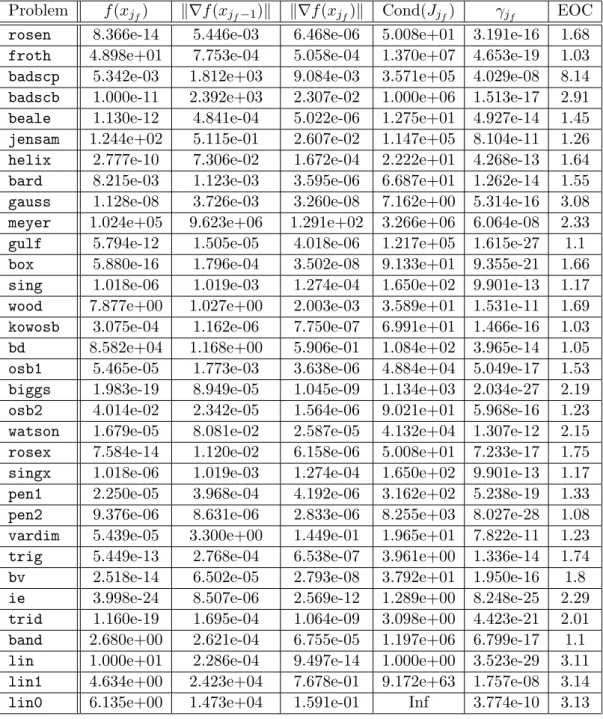
The outline of this paper is as follows. In Section 2 we present the proposed Levenberg- Marquadt algorithm for solving general nonlinear least squares problems. Section 3 addresses the inexact solution of the linearized least squares subproblems arising within the Levenberg- Marquardt method. In Section 4, we show the global convergence of our algorithm. In Section 5 we derive the overall local convergence analysis of the proposed algorithm. In Section 6, preliminary numerical experiments with basic implementations are presented that show the good behavior of our novel algorithm. Finally, in Section 7 we draw some perspectives and conclusions.

Throughout this paper k · k will denote the vector or matrix l ₂ -norm.

2 A novel Levenberg-Marquadt algorithm

In deciding whether to accept a step s j generated by the subproblem (2), the Levenberg- Marquardt method can be seen as precursor of the trust-region method [3]. In fact, it seeks to determine when the Gauss-Newton step is applicable (in which case the regularization param- eter is set to zero) or when it should be replaced by a slower but safer steepest descent step (corresponding to a sufficiently large regularization parameter). For that purpose, one considers the ratio between the actual reduction f (x _j ) − f (x _j + s _j ) attained in the objective function and the reduction m j (x j ) − m j (x j + s j ) predicted by the model, given by

ρ _j = f(x _j ) − f (x _j + s _j ) m _j (x _j ) − m _j (x _j + s _j ) .

Then, if ρ j is sufficiently above zero, the step is accepted and γ j is possibly decreased. Otherwise the step is rejected and γ _j is increased.

In this paper we consider the choice of the regularization parameter as γ j = µk∇f (x j )k ² . where µ is updated according to the ratio ρ j . The considered Levenberg-Marquardt algorithm is described below.

Algorithm 1: Levenberg-Marquardt algorithm.

Initialization

Choose the constants η ∈ (0, 1), µ _min > 0 and λ > 1. Select x ₀ and µ ₀ ≥ µ _min . Set γ 0 = µ 0 k∇f(x ₀ )k ² and ¯ µ = µ 0 .

For j = 0, 1, 2, . . .

1. Solve (or approximately solve) (2), and let s j denote such a solution.

2. Compute ρ j = _m ^f(x

^)−f(x

^+s

⁾

j

(x

)−m

(x

+s

) .

3. If ρ j ≥ η, then set x j+1 = x j + s j and µ j+1 ∈ [max(µ min , µ/λ), ¯ µ] and ¯ ¯ µ = µ j+1 . Otherwise, set x _j+1 = x _j and µ _j+1 = λµ _j .

4. Compute γ _j+1 = µ _j+1 k∇f (x _j+1 )k ² .

A brief remark is warranted regarding the new step acceptance criteria. Note that we have

an auxiliary parameter ¯ µ, that represents the last good parameter. This is necessary in order to

balance the requirements of global and local convergence. If the model is relatively inaccurate, then µ j is driven higher, however, when we reach a region of local convergence, we need the parameter γ _j to encourage local convergence, and thus bound µ _j so that the component k∇f (x)k dominates the behavior of the parameter γ _j . It can be seen that the convergence theory does not change with some heuristic modifications of the procedure to prevent an unnecessarily large number of iterations out of an inaccurate approximation far from the solution to increase µ after a lucky step that brings it back down to ¯ µ, e.g., by saving the last high value of µ _j upon a successful step, and coming back to it if the next step is indeed poor.

3 Inexact solution of the linearized subproblems

Step 1 of Algorithm 1 requires the approximate solution of subproblem (2). As in trust-regions methods, there are different techniques to approximate the solution of this subproblem yielding a globally convergent step. For the purposes of global convergence it is sufficient to compute a step s j that provides a reduction in the model as good as the one produced by the so-called Cauchy step (defined as the minimizer of the model along the negative gradient).

The Cauchy step is defined by minimizing m _j (x _j − t∇f (x _j )) when t > 0 and is given by s c

j = − k∇f (x _j )k ²

∇f (x _j ) ^> (J _j ^> J _j + γ _j I)∇f (x _j ) ∇f (x _j ). (3) The corresponding Cauchy decrease of the model is

m j (x j ) − m j (x j + s c

j ) = 1 2

k∇f (x j )k ⁴

∇f(x _j ) ^> (J _j ^> J _j + γ _j I)∇f (x _j ) . Since ∇f(x _j ) ^> (J _j ^> J _j + γ _j I)∇f (x _j ) ≤ k∇f(x _j )k ² (kJ _j k ² + γ _j ), we conclude that

m _j (x _j ) − m _j (x _j + s c

j ) ≥ 1 2

k∇f (x _j )k ² kJ _j k ² + γ _j .

The Cauchy step (3) is cheap to calculate as it does not require any system solve. Moreover, the Levenberg-Marquadt method will be globally convergent if it uses a step that attains a reduction in the model as good as a multiple of the Cauchy decrease. Thus we will impose the following assumption on the step calculation:

Assumption 3.1 For every step j,

m _j (x _j ) − m _j (x _j + s _j ) ≥ θ _{f cd} 2

k∇f (x _j )k ² kJ _j k ² + γ _j for some constant θ _{f cd} > 0.

Despite providing a sufficient reduction in the model and being cheap to compute, the Cauchy

step is a particular form of steepest descent. In practice, a version of Algorithm 1 solely based

on the Cauchy step would suffer from the same drawbacks as the steepest descent algorithm on

ill-conditioned problems. One can see that the Cauchy step depends on J _j ^> J j only in the step

length. Faster convergence can be expected if the matrix J _j ^> J _j also influences the step direction.

Since the Cauchy step is the first step of the conjugate gradient method (CG) when applied to the minimization of the quadratic s → m j (x j + s), it is natural to propose to run the CG further and stop only when the residual becomes relatively small. The truncated-CG step is of the form:

s cg

j = V j

V _j ^> (J _j ^> J j + γ j I )V j

−1

V _j ^T ∇f (x j ), (4) where V _j is a given unitary matrix whose first column is given by −∇f(x _j )/k∇f (x _j )k.

Since the CG generates iterates by minimizing the quadratic model over nested Krylov subspaces, and the first subspace is the one generated by ∇f (x _j ) (see, e.g., [14, Theorem 5.2]), the decrease attained at the first CG iteration (i.e., by the Cauchy step) is kept by the remaining iterations. Thus Assumption 3.1 holds for all the iterates s cg

j generated by the truncated-CG.

The following Lemma is similar to [1, Lemma 5.1] and will be useful for our global convergence analysis.

Lemma 3.1 For the three steps proposed (exact, Cauchy, and truncated-CG), one has that

ks _j k ≤ k∇f (x _j )k γ j

= 1

µ j k∇f (x j )k and

|s ^> _j (γ _j s _j + ∇f (x _j ))| ≤ kJ _j k ² k∇f (x j )k ²

γ _j ² = kJ _j k ² µ ² _j k∇f (x j )k ² .

Proof. We will omit the indices j in the proof. We note that the truncated-CG step can be seen as a generalized step of both exact and Cauchy steps. In fact, the first CG iteration produces the Cauchy step while the last iteration gives the exact one.

Thus, without loss of generality, for the three proposed steps there exists a unitary matrix V with first column given by −∇f (x)/k∇f (x)k and such that

s = V

V ^> (J ^> J + γI)V −1

V ^T ∇f (x) = V

V ^> J ^> J V + γI −1

k∇f (x)ke ₁ ,

where e ₁ is the first vector of the canonical basis of R ⁿ . From the positive semidefiniteness of V ^> J ^> J V , we immediately obtain ksk ≤ k∇f (x)k/γ.

To prove the second inequality of Lemma 3.1, we apply the Sherman–Morrisson–Woodbury formula and obtain

s = V 1 γ I − 1

γ ² (J V ) ^>

I + (J V )(J V ) ^>

γ

−1

(J V )

!

k∇f (x)ke ₁ . Since V e ₁ = −∇f (x)/k∇f (x)k,

γs + ∇f (x) = − 1

γ V (J V ) ^>

I + (J V )(J V ) ^>

γ

⁻¹

(J V )k∇f (x)ke ₁ .

Now, from the fact that (J V )(J V ) ^> /γ is positive semidefinite, the norm of the inverse of I + (J V )(J V ) ^> /γ is less than one, and thus (since V is unitary)

kγs + ∇f (x)k ≤ kJ k ² k∇f (x)k

γ .

Finally,

|s ^> (γs + ∇f(x))| ≤ kskkγs + ∇f (x)k ≤ kJ k ² k∇f(x)k ² γ ² .

4 Global convergence

We start by giving some classical assumptions and then state and prove some lemmas that later will appear in the global convergence analysis.

Assumption 4.1 The function f is continuously differentiable in an open set containing L(x 0 ) = {x ∈ R ⁿ : f(x) ≤ f (x 0 )} with Lipschitz continuous gradient on L(x 0 ) and corresponding constant ν > 0.

Assumption 4.2 The function f gradient is uniformly bounded, i.e., there exists κ _g > 0 such that k∇f (x j )k ≤ κ g for all j.

Assumption 4.3 The function F Jacobian is uniformly bounded, i.e., there exists κ _J > 0 such that kJ _j k ≤ κ _J for all j.

The next lemma says that, if we suppose that the gradient norm is bounded below by a non zero constant g min , then for a value of the parameter µ j sufficiently large, the step is accepted by the acceptance criterion.

Lemma 4.1 Let Assumptions 3.1, 4.1, 4.2, and 4.3 hold. Suppose that, for all the iterations j, there exists a bound g min > 0 such that k∇f (x j )k ≥ g min . Then , one has

µ

lim →∞ ρ j = 2.

Proof. By applying a Taylor expansion, one has 1 − ρ j

2 = m(x j ) − f (x j ) + f(x j + s j ) − m(x j + s j ) + m(x j ) − m(x j + s j ) 2[m(x _j ) − m(x _j + s _j )]

= R − s ^> _j ∇f (x _j ) − s ^> _j (J _j ^> J _j + γ _j I)s _j 2[m(x j ) − m(x j + s j )]

= R − s ^> _j (J _j ^> J j )s j − s ^> _j (γ j s j + ∇f(x _j ))

2[m(x _j ) − m(x _j + s _j )] where R ≤ ν

2 ksk ² .

Then, using Lemma 3.1, Assumptions 3.1 and 4.1, one gets

|1 − ρ j

2 | ≤

ν

2 ks _j k ² + kJ _j k ² ks _j k ² + |s ^> _j (γ j s j + ∇f (x j ))|

θ

k∇f (x

)k

kJ

k

+γ

≤

ν

2 + 2κ ² _J θ _{f cd}

κ ² _J + γ j

γ _j ²

≤

ν

2 + 2κ ² _J θ _{f cd}

κ ² _J + µ j k∇f (x j )k ² µ ² _j k∇f (x _j )k ⁴

≤

ν

2 + 2κ ² _J θ _{f cd}

κ ² _J + µ _j κ ² _g µ ² _j g ⁴ _min .

Now, we can show our main global convergence result

Theorem 4.1 Under Assumptions 3.1, 4.1, 4.2, and 4.3, the sequence {x _j } generated by Al- gorithm 1 satisfies

lim inf

j→∞ k∇f (x _j )k = 0.

Proof. By contradiction, if the theorem is not true, then there exists a bound g _min > 0 such that

k∇f (x _j )k ≥ g _min , ∀j ≥ 0.

Define S = {j ∈ N | ρ _j ≥ η} as the set of successful iterations. Hence for j ∈ S , one has kF _j k ² − kF _j+1 k ² ≥ η(m j (x j ) − m j (x j + s j ))

≥ η θ _{f cd} 2

k∇f (x _j )k ² kJ _j k ² + γ j

(using Assumption 3.1)

≥ ηθ _{f cd} 2

k∇f(x _j )k ² κ ² _J + µ j k∇f (x j )k ²

≥ ηθ _{f cd} 2

g _min ² κ ² _J + µ _j κ ² _g If S is infinite, then since P

j∈ S kF _j k ² − kF _j+1 k ² is finite, we deduce that

j→∞ lim ηθ f cd

2

g _min ²

κ ² _J + µ _j κ ² _g = 0, hence lim j→∞ µ _j = +∞.

Otherwise (i.e., S is finite), from Algorithm 1 we have µ _j+1 = λµ _j for all sufficiently large j.

Since λ > 1, we deduce that lim j→∞ µ j = +∞.

Thus, using Lemma 4.1, we have lim j→∞ ρ _j = 2. Since when ρ _j ≥ η we decrease µ _j then,

there exists a positive constant µ _max such that µ _j ≤ µ _max holds for all sufficiently large j. Which

leads to a contradiction with the fact that µ j goes to infinity when j goes to +∞.

5 Local convergence

In this section we present the local convergence analysis of Algorithm 1. In particular, we show a quadratic convergence rate without assuming the nonsingularity of J(x). As mentioned in Section 1, the state of the art for problems with zero residual at the solution is that local convergence at a quadratic rate holds under a Lipschitz continuity and error bound assumptions.

We will replicate this in a manner appropriate for problems without a zero residual at the solution. In the sequel of this section, the considered step is the exact solution of subproblem (2).

5.1 Assumptions

In this setting, kF (x)k is no longer an appropriate measure for the distance to the solution.

Stationarity is associated with a zero gradient, and, as can be gleaned from the form of our update for the regularization parameter γ _j in Algorithm 1, this is what we use for the regularization to encourage fast convergence.

In the case of zero-residual problems, there is a set of solutions to F (x) = 0 and the purpose of the algorithm is to obtain a point at which the residual is zero. In this case, we seek a stationary solution where ∇f (x) = 0, however there can be multiple sets of stationary points, with varying objective values. As the behavior of the algorithm is such that both descent of f(x) encouraged as well as a solution to stationarity is sought, for a clear picture of the convergence, we instead propose to consider a particular subset with a constant value of the objective.

Assumption 5.1 There exists a connected isolated set X ^∗ composed of stationary points to (1), and Algorithm 1 generates a sequence with an accumulation point x ^∗ ∈ X ^∗ .

We shall denote by ¯ F the value of ¯ F = kF (¯ x)k at any ¯ x ∈ X ^∗ . Note that this is unique, as X ^∗ is a connected set of stationary points, so there is no direction of ascent for f(x) among the set of directions feasible within X ^∗ .

Henceforth, from the global convergence analysis, we can assume, without loss of generality, that there exists a subsequence approaching this X ^∗ . This subsequence need not be unique, i.e., there may be more than one subsequence converging to separate connected sets of stationary points. We shall see that eventually, one of these sets shall ”catch” the subsequence and result in direct convergence to the solution set at a quadratic rate.

In the sequel N (x, δ) denotes the closed ball of center x (a given vector) and radii δ > 0.

dist(x, X ^∗ ) denotes the distance between the vector x and the set X ^∗ , dist(x, X ^∗ ) = min y∈X

kx−

yk.

Assumption 5.2 It holds that F (x) and J(x) are both locally Lipschitz continuous around x ^∗ ∈ X ^∗ with x ^∗ satisfying Assumption 5.1. In particular this implies, letting x ¯ = argmin _y∈X

kx−yk, that there exists δ 1 > 0 such that for x ∈ N (x ^∗ , δ 1 ),

k∇f (x)k ² = kF (x)J (x)k ² = kF (x)J(x) − F(¯ x)J (¯ x)k ² ≤ L ₁ dist(x, X ^∗ ) ² , (5) kF (x) − F (¯ x)k ≤ L ₂ dist(x, X ^∗ ), (6) and that for all x, y ∈ N (x ^∗ , δ),

kF (y) − F (x) − J (x)(y − x)k ≤ L 3 ky − xk ² , (7)

where L ₁ , L ₂ , and L ₃ are positive constants.

From the triangle inequality and assuming (6), we get

kF (x)k − F ¯ ≤ kF (x) − F (¯ x)k ≤ L ₂ dist(x, X ^∗ ). (8) In addition, as it would be standard for unconstrained optimization, the gradient gives an error bound for the distance to the solution,

Assumption 5.3 There exists a δ ₂ > 0 and M ₁ > 0 such that for x ∈ N (x ^∗ , δ ₂ ), dist(x, X ^∗ ) ≤ M ₁ k∇f (x)k.

However, this is insufficient for local convergence analysis. If the gradient is the only error bound, then in order to ensure local convergence, an accurate second derivative approximation must be available to quadratically reduce the error bound. This can be seen from the care- ful analysis in [7, 6] of local convergence for a family of Newton methods for problems with nonisolated solutions. Since the Levenberg-Marquadt method is based on the Gauss-Newton approximation eschewing calculation of the second derivatives of F (x), this suggests that the gradient would be unsatisfactory.

Thus we introduce an additional assumption,

Assumption 5.4 There exists a δ 3 > 0 and M 2 > 0 such that for x ∈ N (x ^∗ , δ 3 ), dist(x, X ^∗ ) ≤ M 2 (kF(x)k − F). ¯

Note the resemblance to the zero residual case [19, 9, 5, 6]. If ¯ F = 0 then the usual error bound assumption is recovered. In addition, locally, nonsingularity of J(x) or standard second order sufficient optimality conditions imply this error bound.

5.2 Convergence Proof

From the global convergence results, we have established that there is a subsequence of suc- cessful iterations converging to a solution set X ^∗ . In this section, we begin by considering the subsequence of iterations that succeed the successful iterations, i.e., we consider the subsequence K = {j + 1 : j ∈ S }. We shall present the results with a slight abuse of notation that simplifies the presentation without sacrificing accuracy or generality: in particular every time we denote a quantity a _j , the index j corresponds to an element of this subsequence K denoted above, thus when we say a particular statement holds eventually, this means that it holds for all j ∈ S + 1 with j sufficiently large.

We shall denote ˆ µ as an upper bound for ¯ µ. Note that this exists for {µ _j } _j∈K by the formulation of Algorithm 1. In addition we shall denote δ as δ = min(δ 1 , δ 2 , δ 3 ), with {δ _i } _i=1,2,3 defined in the Assumptions.

In the proof we follow the structure of the local convergence proof in [19], with the additional point that the step is accepted by the globalization procedure. We define,

¯

x _j = argmin _y∈X

kx _j − yk.

This Lemma is similar to [19, Lemma 2.1].

Lemma 5.1 Suppose Assumptions 5.2, 5.3, and 5.4.

If x j ∈ N (x ^∗ , ^δ ₂ ), then the solution s j to (2) satisfies,

kJ _j s _j + F _j k − F ¯ ≤ C ₁ dist(x _j , X ^∗ ) ² , (9) where C ₁ is a positive constant independent of j.

Proof. We have,

kJ _j s _j + F _j k ² ≤ 2m _j (s _j ) ≤ 2m _j (¯ x _j − x _j ) = kJ _j (¯ x _j − x _j ) + F _j k ² + γ _j k¯ x _j − x _j k ²

≤ kJ _j (¯ x j − x j ) + F j k ² + µ j L 1 kx _j − x ¯ j k ⁴ (using Assumption 5.2)

(a)

≤

F ¯ + L ₃ kx _j − x ¯ _j k ² 2

+ µ _j L ₁ kx _j − x ¯ _j k ⁴

= L ² ₃ + µ _j L ₁ )

x _j − x ¯ _j k ⁴ + 2L ₃ F ¯ kx _j − x ¯ _j k ² + ¯ F ²

≤ L ² ₃ + µ _j L ₁ )

x _j − x ¯ _j k ⁴ + 2L ₃ s

L ² ₃ + µ j L 1

L ² ₃

F ¯ kx _j − x ¯ _j k ² + ¯ F ²

!

= q

L ² ₃ + ˆ µL ₁ kx _j − x ¯ _j k ² + ¯ F 2

where (a) is from the triangle inequality as well as Assumption 5.2, i.e., kJ _j (¯ x _j − x _j ) + F _j k ≤ F ¯ + kJ _j (¯ x _j − x _j ) + F _j − F (¯ x)k

≤ F ¯ + L ₃ kx _j − x ¯ _j k ² .

Lemma 5.2 Suppose Assumptions 5.2, 5.3, and 5.4.

If x _j ∈ N (x ^∗ , ^δ ₂ ), then the solution s _j to (2) satisfies,

ks _j k ≤ C 2 dist(x j , X ^∗ ), (10)

where C ₂ is a positive constant independent of j.

Proof. The solution of the classical Levenberg-Marquadt subproblem, for zero-residual problems proposed in [19] , when solving F (x) − F (¯ x) = 0, satisfies

argmin _s ¹ ₂ kF _j − F (¯ x) + J j sk ² + ¹ ₂ µ j kF _j − F(¯ x)k ² ksk ² ,

= argmin _s ¹ ₂

2F _j ^T J j s − 2F (¯ x) ^T J j s + s ^T J _j ^T J j s + µ j kF _j − F (¯ x)k ² s ^T s

From [19, Lemma 2.1] it holds that the solution to this problem, ˆ s _j , satisfies kˆ s _j k ≤ C ˆ dist(x _j , X ^∗ ), where ˆ C is a positive constant independent of j.

Now define the function

G(s, u ⁽¹⁾ , u ⁽²⁾ ) = 1 2

2F _j ^T J _j s + (u ⁽¹⁾ ) ^T s + s ^T J _j ^T J _j s + u ⁽²⁾ s ^T s

. (11)

We may consider the model in (2) as a perturbation of (11) if we set in the expression of G, u ⁽¹⁾

and u ⁽²⁾ to u ⁽¹⁾ ₀ = 0 and u ⁽²⁾ ₀ = γ _j , respectively. The classical Levenberg-Marquadt model is the

same as (11) with u ⁽¹⁾ ₁ = −2F (¯ x) ^T J j and u ⁽²⁾ ₁ = µ j kF _j − F (¯ x)k ² . In other words, if we change in the expression of G, u ⁽¹⁾ ₁ and u ⁽²⁾ ₁ by u ⁽¹⁾ ₀ and u ⁽²⁾ ₀ , respectively, we modify the model from the classical Levenberg-Marquadt subproblem for zero residual problems to the one defined in (2).

Since the function G is quadratic with respect to s and linear with respect to u, the conditions of [2, Proposition 4.36] are satisfied, and thus,

ks _j − s ˆ _j k ≤ C ˆ ₂ ku ⁽¹⁾ ₁ − u ⁽¹⁾ ₀ k + ˆ C ₃ ku ⁽²⁾ ₁ − u ⁽²⁾ ₀ k

≤ 2 ˆ C ₂ kF (¯ x) ^T J _j k + ˆ C ₃ µ _j |kF _j − F (¯ x)k ² − kF _j J _j k ² |

≤ 2 ˆ C ₂ (kF _j J _j k + kF _j − F(¯ x)kkJ _j k) + ˆ C ₃ max(L ₁ , L ² ₂ )ˆ µ dist(x _j , X ^∗ ) ²

≤ 4 ˆ C ₂ max( p

L ₁ , B _J L ₂ ) dist(x _j , X ^∗ ) + ˆ C ₃ max(L ₁ , L ² ₂ )ˆ µ dist(x _j , X ^∗ ) ²

≤ C ˆ 4 dist(x j , X ^∗ ),

where ˆ C 2 , ˆ C 3 and ˆ C 4 are positive constants independent of j. The second inequality follows from Assumption 5.2, the triangle and Cauchy-Schwartz inequalities, and the final inequality again follows from Assumption 5.2 and the boundedness of J _j by B _J (due to the convergence of x j ).

Thus, from the triangle inequality,

ks _j k ≤ kˆ s j k + ks _j − ˆ s j k ≤ C ˆ + ˆ C 4

dist(x j , X ^∗ ).

Lemma 5.3 For j sufficiently large, ρ j ≥ η.

Proof. Consider first the case of ¯ F > 0.

It holds that,

m _j (x _j ) − m _j (x _j + s _j ) = kF _j k ² − kF _j + J _j s _j k ² − γ _j ks _j k ²

(a)

≥ kF _j k ² − kF _j + J j (¯ x j − x j )k ² − γ j k¯ x j − x j k ²

= (kF _j k + kF _j + J j (¯ x j − x j )k) (kF _j k − kF _j + J j (¯ x j − x j )k) − γ j k¯ x j − x j k ²

≥ (kF _j k + kF _j + J j (¯ x j − x j )k) kF _j k − F ¯ − L 3 k¯ x j − x j k ²

− γ j k¯ x j − x j k ²

(b)

≥ kF _j k L ₂ k¯ x _j − x _j k − L ₃ k¯ x _j − x _j k ²

− γ _j k x ¯ _j − x _j k ²

≥ F L ¯ 2 k¯ x j − x j k − (F 0 L 3 + γ j ) k¯ x j − x j k ²

= F L ¯ ₂ k¯ x _j − x _j k −

L ˜ ₃ + γ _j

k¯ x _j − x _j k ² ,

where (a) arises from the optimality of s _j for m _j , and for (b) we note that for j sufficiently large

k¯ x j − x j k ² k¯ x j − x j k and thus L 2 k¯ x j − x j k − L 3 k¯ x j − x j k ² ≥ 0.

Now we write,

|1 − ρ j | =

m(x j ) − f (x j ) + f (x j + s j ) − m(x j + s j ) m(x j ) − m(x j + s j )

=

kF(x _j + s _j )k ² − kF _j + J _j s _j k ² − γ _j ks _j k ² m(x j ) − m(x j + s j )

=

(kF (x _j + s _j )k − kF _j + J _j s _j k) (kF (x _j + s _j )k + kF _j + J _j s _j k) − γ _j ks _j k ² m(x j ) − m(x j + s j )

≤ L 3 ks _j k ² (kF _j k + kJ _j kks _j k) + γ j ks _j k ² F L ¯ ₂ k¯ x _j − x _j k −

L ˜ ₃ + γ _j

k¯ x _j − x _j k ²

→ 0 when j goes to +∞.

The last limit is zero because ks _j k = O(kx _j − x ¯ _j k) → 0 by Lemma 5.2, γ _j is bounded, and F > ¯ 0.

Now, if ¯ F = 0, we have, from the same derivation, m _j (x _j ) − m _j (x _j + s _j ) ≥ kF _j kL ₂ k¯ x _j − x _j k −

L ˜ ₃ + γ _j

k¯ x _j − x _j k ² ,

and, using Assumptions 5.4 and 5.2 as well as Lemma 5.2,

|1 − ρ j | ≤ L 3 ks _j k ² (kF _j k + kJ _j kks _j k) + γ j ks _j k ² kF _j kL ₂ k¯ x _j − x _j k −

L ˜ ₃ + γ _j

k¯ x _j − x _j k ²

≤ C ₅ kx _j − x ¯ _j k ² (kx _j − x ¯ _j k + kJ _j kkx _j − x ¯ _j k) + γ _j kx _j − x ¯ _j k ² L ˜ ₂ kx _j − x ¯ _j kk¯ x _j − x _j k −

L ˜ ₃ + γ _j

k¯ x _j − x _j k ² ,

and thus the power for kx _j − x ¯ j k is larger in the numerator and the fraction converges to zero.

This next Lemma is similar to [19, Lemma 2.2].

Lemma 5.4 Suppose Assumptions 5.2, 5.3, and 5.4.

If x _j , x _j+1 ∈ N (x ^∗ , δ/2), then,

dist(x j+1 , X ^∗ ) ≤ C 3 dist(x j , X ^∗ ) ² , (12) where C 3 is a positive constant independent of j.

Proof. Indeed,

dist(x j+1 , X ^∗ ) ² ≤ dist(x j + s j , X ^∗ ) ² ≤ M ₂ ² (kF(x _j + s j )k − F ¯ ) ²

≤ M ₂ ² kJ (x j )s j + F j k + L 3 ks _j k ² − F ¯ 2

≤ M ₂ ² C 1 kx _j − x ¯ j k ² + ¯ F + L 3 C ₂ ² kx _j − x ¯ j k ² − F ¯ 2

≤ M ₂ ² C ₁ + L ₃ C ₂ ² 2

dist(x _j , X ^∗ ) ⁴ ,

where we used Lemma 5.1 in the second to last inequality.

Theorem 5.1 Algorithm 1 converges locally quadratically to X ^∗ .

Proof. From the previous results, it can be seen that eventually for j ∈ K = S + 1, it holds that there is a step s j such that x j + s j is quadratically closer to the solution, and is accepted.

In particular, by the same argument as given in [19, Lemma 2.3] x _j + s _j is always at least as close to x ^∗ as x j , and thus x j+1 = x j + s j lies in a ball around x ^∗ for which all of the local assumptions hold as well.

But then this implies that j + 1 ∈ K as well, and all of the previous results apply to it.

Thus, proceeding inductively we get that for sufficiently large j ∈ K, it holds that all subsequent iterations are in K and the entire sequence of iterates {x _j } (no longer subsequence) locally converges quadratically to X ^∗ .

6 Numerical results

In this section we present some results of numerical experiments performed implementing Al- gorithm 1. We performed our experiments using the well known 33 Mor´ e/Garbow/Hillstrom test problems [13]. All the tested problems are smooth and have a least-squares structure. The residual function F and the Jacobian matrix for all the test problems [13] are implemented in MATLAB. Some of these problems have a non-zero value at the optimum and thus are consistent with the scope of the paper. In what comes next, we refer to the Mor´ e/Garbow/Hillstrom test problems by P .

Among all the test problems in P three problems can be seen as ill-conditioned (meaning that the condition number of their Jacobian at the optimum is larger than 10 ⁷ ). Two of them are even nearly singular (i.e., the condition number of their Jacobian at the optimum is larger than 10 ²⁰ ). For all the tested problems, we used the proposed starting points x 0 as in the original optimization test problems [13].

A preliminary implementation of Algorithm 1 was written in MATLAB. The initial param- eters defining the implemented algorithm were set as follows:

η = 0.01, λ = 2, µ ₀ = 1, µ _min = 10 ⁻¹⁶ .

At each iteration of Algorithm 1 we solved exactly the subproblem using the backslash MATLAB operator. If the iteration successful, we set the parameter µ _j+1 equals to max(¯ µ/λ, µ _min ). The algorithm is stopped when

k∇f(x _j )k ≤ max(1, k∇f(x ₀ )k) with = 10 ⁻⁵ .

If it did not converge within a maximum number of iterations j max = 10000, then Algorithm 1 was considered to have failed.

The order of convergence was estimated by the quantity EOC = log

k∇f (x _j

)k max(1, k∇f (x ₀ )k)

/ log

k∇f (x _j

−1 )k max(1, k∇f (x ₀ )k)

, (13)

where j _f denotes the index of the final computed iterate. The obtained values of EOC will help

to estimate the speed of convergence. For the problems with an EOC ≥ 1.8 Algorithm 1 will

be said to be quadratically converging. For test problems with 1.8 > EOC ≥ 1.1 the algorithm

Table 1: Order of convergence distribution all over P . Order of convergence

Total Linear or Sub-linear Super-linear Quadratic

Well-conditioned 3 17 10 30

Poorly conditioned 1 0 2 3

Total 4 17 12 33

Table 2: The complete results for Algorithm 1 on the tested problems.

Problem f (x j

) k∇f (x j

−1 )k k∇f (x j

)k Cond(J j

) γ j

EOC

rosen 8.366e-14 5.446e-03 6.468e-06 5.008e+01 3.191e-16 1.68

froth 4.898e+01 7.753e-04 5.058e-04 1.370e+07 4.653e-19 1.03

badscp 5.342e-03 1.812e+03 9.084e-03 3.571e+05 4.029e-08 8.14

badscb 1.000e-11 2.392e+03 2.307e-02 1.000e+06 1.513e-17 2.91

beale 1.130e-12 4.841e-04 5.022e-06 1.275e+01 4.927e-14 1.45

jensam 1.244e+02 5.115e-01 2.607e-02 1.147e+05 8.104e-11 1.26

helix 2.777e-10 7.306e-02 1.672e-04 2.222e+01 4.268e-13 1.64

bard 8.215e-03 1.123e-03 3.595e-06 6.687e+01 1.262e-14 1.55

gauss 1.128e-08 3.726e-03 3.260e-08 7.162e+00 5.314e-16 3.08

meyer 1.024e+05 9.623e+06 1.291e+02 3.266e+06 6.064e-08 2.33

gulf 5.794e-12 1.505e-05 4.018e-06 1.217e+05 1.615e-27 1.1

box 5.880e-16 1.796e-04 3.502e-08 9.133e+01 9.355e-21 1.66

sing 1.018e-06 1.019e-03 1.274e-04 1.650e+02 9.901e-13 1.17

wood 7.877e+00 1.027e+00 2.003e-03 3.589e+01 1.531e-11 1.69

kowosb 3.075e-04 1.162e-06 7.750e-07 6.991e+01 1.466e-16 1.03

bd 8.582e+04 1.168e+00 5.906e-01 1.084e+02 3.965e-14 1.05

osb1 5.465e-05 1.773e-03 3.638e-06 4.884e+04 5.049e-17 1.53

biggs 1.983e-19 8.949e-05 1.045e-09 1.134e+03 2.034e-27 2.19

osb2 4.014e-02 2.342e-05 1.564e-06 9.021e+01 5.968e-16 1.23

watson 1.679e-05 8.081e-02 2.587e-05 4.132e+04 1.307e-12 2.15

rosex 7.584e-14 1.120e-02 6.158e-06 5.008e+01 7.233e-17 1.75

singx 1.018e-06 1.019e-03 1.274e-04 1.650e+02 9.901e-13 1.17

pen1 2.250e-05 3.968e-04 4.192e-06 3.162e+02 5.238e-19 1.33

pen2 9.376e-06 8.631e-06 2.833e-06 8.255e+03 8.027e-28 1.08

vardim 5.439e-05 3.300e+00 1.449e-01 1.965e+01 7.822e-11 1.23

trig 5.449e-13 2.768e-04 6.538e-07 3.961e+00 1.336e-14 1.74

bv 2.518e-14 6.502e-05 2.793e-08 3.792e+01 1.950e-16 1.8

ie 3.998e-24 8.507e-06 2.569e-12 1.289e+00 8.248e-25 2.29

trid 1.160e-19 1.695e-04 1.064e-09 3.098e+00 4.423e-21 2.01

band 2.680e+00 2.621e-04 6.755e-05 1.197e+06 6.799e-17 1.1

lin 1.000e+01 2.286e-04 9.497e-14 1.000e+00 3.523e-29 3.11

lin1 4.634e+00 2.423e+04 7.678e-01 9.172e+63 1.757e-08 3.14

lin0 6.135e+00 1.473e+04 1.591e-01 Inf 3.774e-10 3.13

can be seen as super-linearly converging. Otherwise (i.e., EOC < 1.1 ), Algorithm 1 will be estimated to converge linearly or worse.

Table 1 gives the distribution of the order of convergence over our test set P . The detailed results are presented in Table 2. The obtained results confirm our theoretical analysis in two senses. First, for all the tested problems, we observe the global convergence of our proposed algorithm. Second, we obtain quadratic or super-linear convergence rates on most of the prob- lems tested. In fact, among the 33 tested problems, only 4 converge linearly or worse, for 12 problems we observe quadratic convergence and 17 are super-linearly converging.

7 Conclusion

In this paper we presented and analyzed a novel Levenberg-Marquadt method for solving non- linear least-squares problems. In particular we were interested in the class of problems for which there is no zero-residual solution (or such a solution is not sought after) and the problem is potentially ill-conditioned. Without the use of ancillary procedures to enforce globalization, we were able to formulate a method that is provably and numerically demonstrably convergent at a quadratic rate for such problems. Future research can include problems with constraints as well as those with noisy data.

References

[1] E. Bergou, S. Gratton, and L. N. Vicente. Levenberg-Marquardt Methods Based on Prob- abilistic Gradient Models and Inexact Subproblem Solution, with Application to Data As- similation. SIAM/ASA J. Uncertainty Quantification, 4:924–951, 2016.

[2] J. F. Bonnans and A. Shapiro. Perturbation Analysis of Optimization Problems. Springer Science & Business Media, 2013.

[3] A. R. Conn, N. I. M. Gould, and Ph. L. Toint. Trust-Region Methods. SIAM, Philadelphia, PA, USA, 2000.

[4] P. Courtier, J.-N Th´ epaut, and A. Hollingsworth. A Strategy for Operational Implementa- tion of 4D-Var, Using an Incremental Approach. Q. J. R. Meteorol. Soc., 120:1367–1388, 1994.

[5] H. Dan, N. Yamashita, and M. Fukushima. Convergence Properties of the Inexact Levenberg-Marquardt Method under Local Error Bound Conditions. Optim. Methods Softw., 17:605–626, 2002.

[6] F. Facchinei, A. Fischer, and M. Herrich. A Family of Newton Methods for Nonsmooth Constrained Systems with Nonisolated Solutions. Math. Methods Operations Research, 77:433–443, 2013.

[7] F. Facchinei, A. Fischer, and M. Herrich. An LP-Newton Method: Nonsmooth Equations, KKT Systems, and Nonisolated Solutions. Math. Program., 146:1–36, 2014.

[8] J. Fan. Convergence Rate of the Trust Region Method for Nonlinear Equations under Local

Error Bound Condition. Comput. Optim. Appl., 34:215–227, 2006.

[9] J. Fan and Y. Yuan. On the Quadratic Convergence of the Levenberg-Marquardt Method without Nonsingularity Assumption. Computing, 74:23–39, 2005.

[10] I. C. F. Ipsen, C. T. Kelley, and S. R. Pope. Rank-deficient Nonlinear Least Squares Problems and Subset Selection. SIAM J. Numer. Anal., 49:1244–1266, 2011.

[11] K. Levenberg. A Method for the Solution of Certain Problems in Least Squares. Quart.

Appl. Math., 2:164–168, 1944.

[12] D. Marquardt. An Algorithm for Least-Squares Estimation of Nonlinear Parameters. SIAM J. Appl. Math., 11:431–441, 1963.

[13] J. J. Mor´ e, B. S. Garbow, and K. E. Hillstrom. Testing Unconstrained Optimization Soft- ware. ACM Trans. Math. Softw., 7:17–41, 1981.

[14] J. Nocedal and S. J. Wright. Numerical Optimization. Springer-Verlag, Berlin, second edition, 2006.

[15] M. R. Osborne. Nonlinear Least Squares – The Levenberg Algorithm Revisited. J. Austral.

Math. Soc. Ser. B, 19:343–357, 1976.

[16] A. Tarantola. Inverse Problem Theory and Methods for Model Parameter Estimation.

SIAM, Philadelphia, 2005.

[17] Y. Tr´ emolet. Model Error Estimation in 4D-Var. Q. J. R. Meteorol. Soc., 133:1267–1280, 2007.

[18] J. Virieux and S. Operto. An Overview of Full-Waveform Inversion in Exploration Geo- physics. Geophysics, 74:WCC1–WCC26, 2009.

[19] N. Yamashita and M. Fukushima. On the Rate of Convergence of the Levenberg-Marquardt

Method. In Topics in numerical analysis, pages 239–249. Springer, 2001.