The acoustics of fricative consonants

The Acoustics of Fricative Consonants

Christine Helen Shadle

Technical Report 506

March 1985

Massachusetts Institute of Technology

Research Laboratory of Electronics

Cambridge, Massachusetts 02139

-f Kq K5,i

CD. 04

, .... X

ENGWEE.pI

Usf"AA,

The Acoustics of Fricative Consonants

Christine Helen Shadle

Technical Report 506

March 1985

Massachusetts Institute of Technology

Research Laboratory of Electronics

Cambridge, Massachusetts 02139

This work has been supported in part by the National Institutes of Health Grant 5 R01 NS04332

fil

1~

L3

I

?

7;I

tk II L U 0 '5

!T. LIBRRE

MAR 1 6 19

i

THE ACOUSTICS OF FRICATIVE CONSONANTS by Christine Helen Shadle

Submitted to the Department of Electrical Engineering and Computer Science on March 21, 1985. in partial fulfillment of the requirements for the degree of Doctor of Philosophy.

ABSTRACT

The acoustic mechanism of fricative consonants was studied in the context of three domains: speech, mechanical models. and theoretical models. All fricative configurations have in common a small turbulence-producing constriction within the vocal tract. Thus, preliminary experiments were conducted using a mechanical model having this basic configuration of a constriction in a tube. Parameters such as constriction area. length. location, and degree of inlet tapering, and presence of an obstacle, were varied. It was found that acoustically the most significant parameters are the presence of an obstacle, the length of the front cavity, and the flowrate. Therefore, configurations in which only these parameters were varied, referred to as the obstacle and no-obstacle cases, were examined more thoroughly and modeled theoretically.

A source function for the obstacle case was derived from the far-field sound pressure mea-sured when the obstacle was located in space, downstream of a constriction in a baffle. The directivity pattern produced by the obstacle in this position was similar to that of a dipole, as expected. A dipole source located inside a duct is equivalent to a pressure source in a transmnission-lille model, when only the longitudinal modes of a duct are considered. The filter function. corresponding to the effect of the duct on such a pressure source, was derived for the transmission-line representations of two configurations in which the obstacle was located inside a front cavity of nonzero length. The spectra predicted by this source-filter model, when compared to the far-field pressure measurements of the equivalent mechanical models, provided a very close match in both absolute sound pressure level and spectral shape. Thus in this case the presence of the duct does not significantly alter the sound source, and a simple linear source-filter model works well.

For the no-obstacle case, it was not possible to derive a source from a free-field measurement, so the validity of a source-tract model could not be checked directly. Investigation of the pressure versus flow-velocity power laws showed evidence of source-tract interaction for the no-obstacle case, but none for the obstacle case.

Spectral measures were developed that characterized the acoustic differences caused by the different types of sources for the obstacle and no-obstacle cases. Analysis of real speech in terms of these spectral measures revealed that fricatives are more similar to the obstacle than to the no-obstacle case. More complex speech-like mechanical models were developed and the acoustic characteristics of the sounds generated by those models were compared to the characteristics of speech sounds, again in terms of the spectral measures. Very good models of /s/ and // were obtained by usilg an obstacle at right angles to the flow and varying the constriction location. For the fricatives /, f. 0/. in which the constriction is located forward in the tract. the shape of the constriction was crucial. Constrictions that allowed the jet tocome in contact with a surface produced sounds that most closely resembled the analyzed eamnples of these fricatives. For /x/ and // in which the constriction is located 4 to 6 cm back from the mouth, a surface also caused the mechanical model spectra to become the most like the speech spectra. However, in general it appears that the constriction shape affects the far-field spectrum less as the front cavity is lengthened. The model for /s, 8/ appears to be that of a series pressure source,

2

located at the teeth. For the fricatives other than /s,3/. a "distributed obstacle", modeled as a distributed pressure source. may be the dominant acoustic mechanism.

The whistles generated by several configurations were also investigated. Orifice tones oc-curred for untapered constrictions. at a greater range of constriction sizes than predicted by previous studies. The frequencies were related to the constriction length. Edgetones occurred for configurations including an obstacle, at frequencies related to the flowrate and distance to the obstacle. The occurrence. frequency and amplitude of the whistle tones were affected by the constriction shape and the presence of a tube surrounding the obstacle.

Edgetones were generated by the /s/- and //-like mechanical models that were similar acoustically to the whistles produced by a subject with the /s/ and // configurations. An even more striking parallel between the whistles produced by speech-like models and humans was found for the typical bilabial whistles produced by //-like configurations. Two constrictions, reproducing the role of tongue and lips, were necessary to model these whistles. The agreement in flow range. frequency, and control parameters of the holetones thus produced and the whistles generated by humans was good enough to suggest that the same acoustic mechanism occurred in both the models and the human vocal tract.

Thesis supervisor: Kenneth N. Stevens

Title: Clarence J. LeBel Professor of Electrical Engineering

3

To

my father

my mother

and my grandmother

for giving me the desire to learn

and

for making it possible

4

Acknowledgments

Doing this thesis has been of necessity a solitary task. yet. paradoxically. a time most richly populated with people. It is with delight that I acknowledge those who helped me in such a variety of ways.

First. I would like to thank Ken Stevens for teaching and advising me patiently and thought-fully. His willingness to let me go off on tangents increased immeasurably the intellectual pleasure I derived from my work; lo and behold, some of the tangents did finally turn into a thesis.

Lou Braida, my graduate counsellor, has also been an indispensable figure of the last six years. Many thanks to him for popping in unexpectedly with interesting and relevant problems and advice, and for concrete assistance in setting up my lab.

The members of my committee, Bill Rabinowitz. Victor Zue. Sheila Widnall, and Uno Ingard, spanned beautifully orthogonal areas of interest and expertise. I thank them for their help and advice, and for reading all those drafts.

I am deeply grateful to Max Mathews, Charles Thompson, and Gunnar Fant. for helping me in a most difficult phase. that of problem definition. Their comments in the beginning stages, as well as later on, greatly influenced my approach.

I wish to thank Rich McGowan, Toni Quatieri., Louis Goldstein, Rich Goldhor, John Wyatt, and Shinji Maeda. who, when asked specific technical questions, took the time to discuss them thoroughly, and taught me a great deal as a result.

Thanks to Patrick Hosein, for his careful work in revising TBFDA; Peter Vitale, for pro-gramming the LSI-11; and Dick Lyon, for his help in designing my muffler. Thanks to Joe Perkell, Larry Frishkopf, and Bob Hillman, for their generosity in lending equipment for "a year" that became two or three. And thanks to Keith North, for explaining the intricacies of tape recording and sound level meters, and finding oscillators at a moments notice. Thanks to Jim Byrne, for teaching me to use a machine shop, and Manny Cabal, for machining all those constrictions.

Special thanks go to the members of the Communication Biophysics Group, for help with an unfamiliar computer system, and for my extensive use of their facilities.

I thank Phyllis Vandermolen and Amy Hendrickson, for their help with figures and text formatting (see, for example, Figure 2.3, and Table 4.2).

Thanks to KS, PP, EM, AS and G for serving as subjects. (Note: upon reading this thesis, you will wonder, who was AS? AS was a subject for a recording session so preliminary that it did not appear in these pages, but for whose time I am nevertheless grateful.)

Many thanks to NIH and the LeBel Foundation. for financial support.

Finally, I want to thank the people who have supported, encouraged and expressed their faith in me so long and well. Among these, I would like especially to thank: Rich Goldhor and Stephanie Seneff. for our thesis-encounter-group lunches that. among other things, helped me to keep a sense of humor: Marie Southwick, Patti Jo Price. and Corine Bickley. for sharing so much with me. and convincing me that there is life during as well as after thesis; Anne Black, John Wyatt, Kent Pitman. Adele Proctor, and Stefanie Shattuck-Hufnagcl. for celebratory dinners, a sense of perspective when I needed it, cookies in the lab at 3 A.M.. and the friendship that made all of that possible; Janet Koelnke, Lorraine Delhornle, Neil Macmillan, Rosalie Uchanski, Diane Bustaniante. Dan Leotta. Tom Lee, Nat Durlach. and the other members of the Communication Biophysics Group at M.I.T., who responded to my use of their facilities

5

with friendship, encouragement, and philosophical discussions, and in general made me feel like an honorary CBG-er; Rosalind Fine. Lois Eichler. John Rust. Yehuda and Joy. for helping me make the most out of the process of being a graduate student: Max Mathews. Sandra Pruzansky, Moise Goldstein, Marcia Bush. Gary Kopec. Karen Landahl. and Emnel Gokcen. for help in spite of being miles away: and my family, Paul. Elinor. Anna and Paula Shadle and Sally and Roger Gottlieb. who found so many ways to tell me to hang in there.

Biographical Note

Christine Shadle was born in Pasadena, California. on February 6, 1954. From age seven onwards she studied classical piano, an interest that became an official avocation when she double-majored in piano performance and electrical engineering at Stanford University. Grad-uating in 1976 with an A.B. and M.S. respectively., she began working with Dr. Bishnu Atal at Bell Telephone Laboratories. Murray Hill. New Jersey, in the Speech and Communications Research Department. Gradually changing focus from computer music to speech analysis and synthesis, she left Bell Labs in January 1979 in order to learn more about the basics of speech research. In February 1979 she became a graduate student of Ken Stevens in the Speech Communications Group of the Department of Electrical Engineering and Computer Science at M.I.T. There she has worked on three main research projects: the intrinsic fundamental fre-quency of vowels in sentence context, the acoustics of whistling, and this thesis, which grew out of the work on whistling. In addition, she was a teaching assistant for courses in probability and acoustics.

Over the last six years, the ups and downs of graduate school have been, shall we say, tem-pered by her habit of playing the preludes and fugues of J.S. Bach's Well-Temtem-pered Clavichord. She currently intends to switch to Bach's Goldberg Variations, to continue research in her thesis area, and to resume her favorite hobbies: chamber music, photography, hiking and sailing.

7

Contents

Abstract Dedication Acknowledgments Biographical Note List of Symbols

1 Introduction and Literature Review

1.1 Introduction .. .. ... ... .... ... ... .... ... ... . 1.2 Literature Review.

1.2.1 General Aspects of Unstable and Turbulent Jets ...

1.2.2 Acoustic Models of Fricatives and Fricative-Like Configurations 1.2.3 Analysis of Fricatives

1.3 Plan of the Thesis ...

2 A Constriction in a Tube: Methodology and Preliminary Experiments

2.1 Method ...

2.1.1 Sound Generating System ... 2.1.2 Sound Analysis System ... 2.1.3 Signal Analysis ...

2.2 Pressure Drop Across a Constriction .... 2.3 Acoustic Results ...

2.3.1 Stable. No-Obstacle Configurations . 2.3.2 Unstable Behavior.

2.3.3 Stable Obstacle Configurations . . . 2.4 Discussion ...

3 The Idealized Obstacle and No-Obstacle Cases

3.1 Theoretical Predictions ...

3.1.1 Source Model for Obstacle Case ... 3.1.2 Tract Models. General Method ... 3.1.3 Low-Frequency Models ... 3.1.4 Higher Frequency Models ... 3.1.5 Final Models. Obstacle Case ... 3.1.6 The No-Obstacle Case ...

3.2 Comparison of Experimental Data and Thcoretical 3.2.1 Method ... 3.2.2 Obstacle Case ... 3.2.3 No-Obstacle Case . ... 3.2.4 Conclusion ... ... .. . . . 27 27 28 29 36 43 43 49 58 59 65 .... ... .. . ... . . 65 . . . 65 ... . ... ... .... . 72 .... . ... .... .... . 81 .... ... .. ... . .. . . 87 ... 100 ... 102 Predictions ... 108 ... . .108 ... .... .109 ... 122 ... 123 8 2 4 5 7 14 17 17 20 20 23 24 25 27

_ ___ _· IIULllrm__lCy___II^- I^U .- -II_-. -.

. . . . . . . . . . . . . . . . . . . . . . . . . . . . . . . . . . . . . . . . . . . . . . . . . . . . . . . . . . . . . . . . . . . . . . . . . . . .

4 Speech and Speech-Like Models

4.1 Speech Analysis. ...

4.1.1 Speech Recording Method. ... 4.1.2 Speech Analysis Method... 4.1.3 Speech Results... 4.2 Speech-like Models. ...

4.2.1 Source due to Obstacle: /s/ and // ...

4.2.2 Short Front Cavity, Source due to Surface: //, /f/, and /0/ 4.2.3 Long Front Cavity, Source due to Surface: // and /x/ . . . 4.2.4 Whistles...

4.3 Discussion... 5 Conclusion

5.1 Summary and Discussion of Results ... 5.2 Future Work ... 128 ... 128 ... 128 ... 129 ... 135 ... 149 ... 149 ... 152 ... 154 ... 165 ... 167 178 ... 178 ... 180

A Establishment of an Absolute Reference Level for the Microphones

B Relationship of Transfer Function Form to Network Topology

C Complete Set of Transfer Functions for the Obstacle Case

D Complete Set of Transfer Functions for the No-Obstacle Case

References 183 184 187 190 192 9 _ I __ _____

List of Figures

1.1 Diagram of a midsagittal cross-section of the vocal tract during the production of the fricative //. The arrow at the tip of the tongue indicates teh point of greatest constriction in the vocal tract. ... ... 18 1.2 Diagram of the mixing, transition and fully developed regions of a fully turbulent

jet ... ... 21

2.1 Diagram of the experimental setup ... . 31 2.2 Averaged pressure spectra of the sound generated by the system upstream of

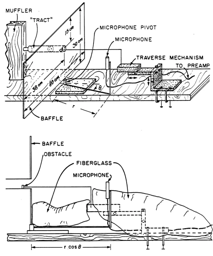
the "tract" with and without the muffler. The dashed line is the curve fit by logarithmic regression to the averaged pressure spectrum of the room noise. For all three curves, number of averages, n, is 16 .. ... 32 2.3 Diagram of the experimental setup downstream of the muffler (top). Expanded

view showing placement of sound-attenuating fiberglass (bottom). Both sketches are not to scale. ... ... 33 2.4 Detailed diagram of the "tract", giving relevant dimensions and the terms used

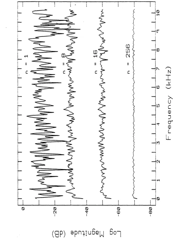
to refer to specific regions . ... 34 2.5 Power spectra of white noise, averaged n times .. .. ... 35 2.6 Curves generated from Heinz' data (1956) for the pressure drop across versus the

volume velocity through a constriction . ... ... 40 2.7 Experimental data for the pressure drop across versus the volume velocity through

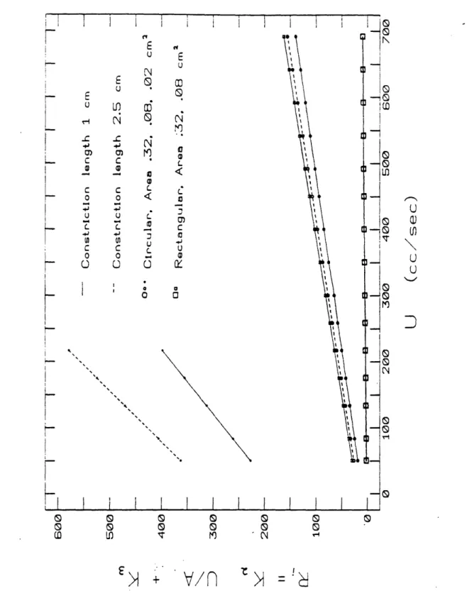
a constriction . . . ... . 41 2.8 Incremental flow resistance of a constriction, versus the volume velocity through

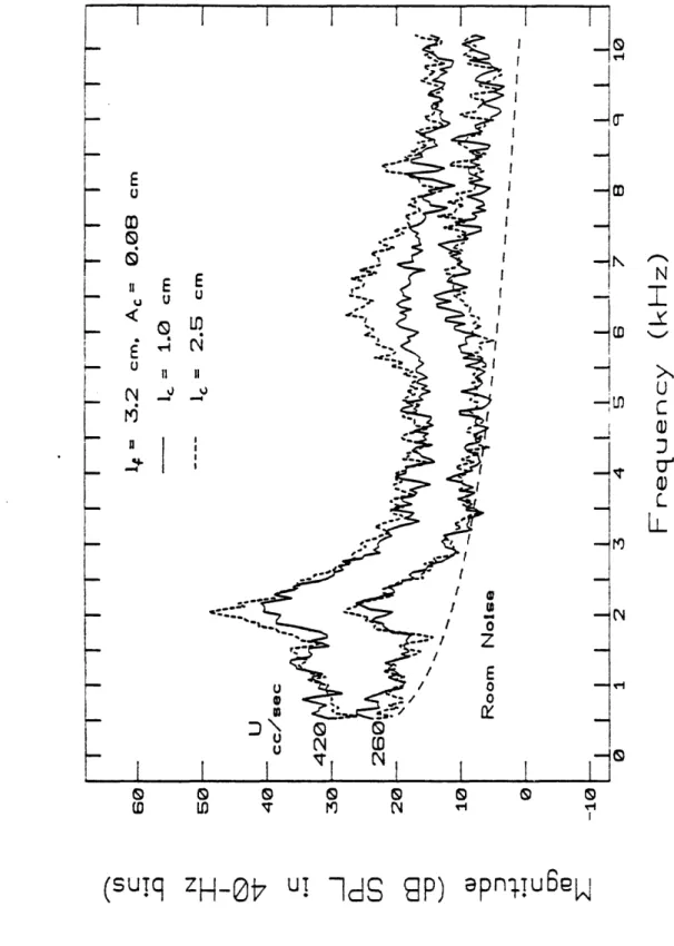
it ... ... ... 42 2.9 Averaged power spectra for front-cavity lengths If = 3.2 and 6 cm, and

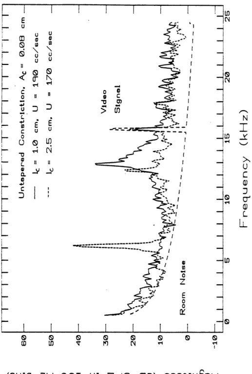
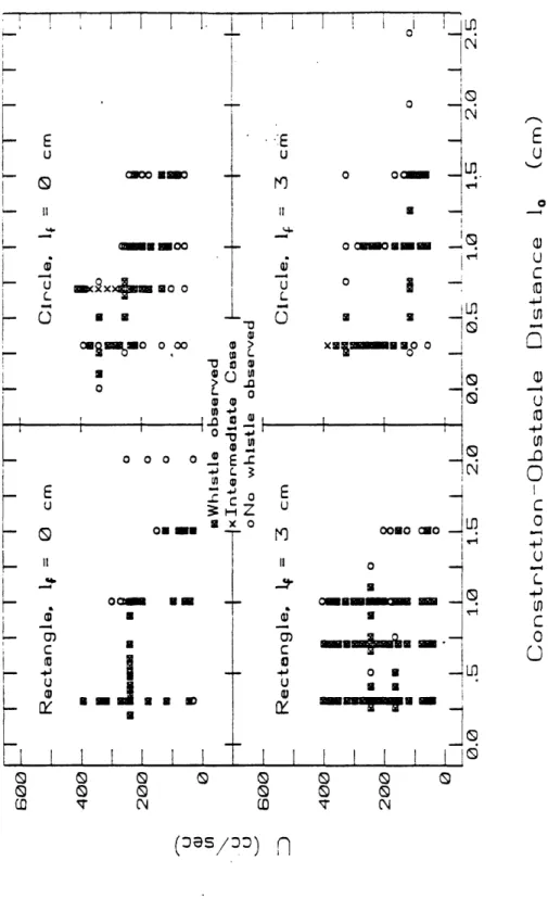
constric-tion areas A, = .08 and .02 cm2... . 46 2.10 Averaged power spectra for I = 3.2 and 6 cm and A, = 0.02, 0.08 and 0.32 cm2. 47 2.11 Averaged power spectra for lc = 1.0 and 2.5 cm . .. ... 48 2.12 Averaged power spectra of untapered constrictions of lengths 1.0 and 2.5 cm . 52 2.13 Summary of the conditions giving rise to whistles for a constriction-obstacle

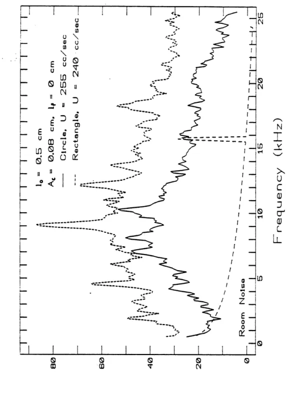
configuration. ... .. .. ... 53 2.14 Typical spectra for the circular and rectangular constrictions at mouth of tube,

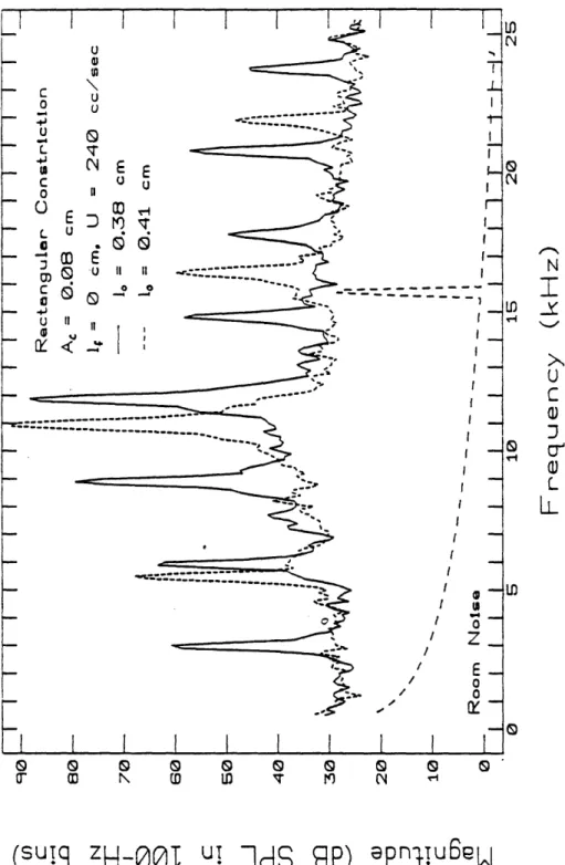
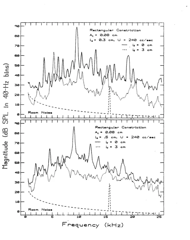
with semicircular obstacle a distance 10o downstream ... 54 2.15 Spectra generated by constriction-obstacle configurations differing only in their

values oflo . . . . ... . 55 2.16 Spectra generated by constriction-obstacle configurations, contrasting length of

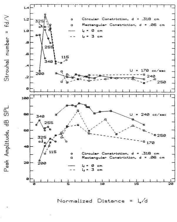
the front cavity at 10 = 0.3 and 0.5 cm. ... 56 2.17 Strouhal number and peak amplitude versus normalized distance to obstacle, for

whistles generated by the constriction-obstacle configuration. ... 57 2.18 Spectra contrasting no-obstacle and non-whistling constriction-obstacle

configu-rations, with all other parameters (, If/, A,) the same. ... 61 2.19 Spectra for non-whistling constriction-obstacle configurations, showing the effect

of variations in 0lo.. . ... . ... 62

10

2.20 Spectra for non-whistling constriction-obstacle configurations. showing the effect of variations in 0...

2.21 Complete directivity patterns for the constriction-obstacle configuration, 10 = 3

cm, If = 0 cm ...

3.1 Diagram of the predictions and comparisons to be made for the obstacle case. 3.2 Schematics of dipole reflected in baffle ...

3.3 Predicted far-field pressure due to three dipoles reflected in baffle, versus fre-quency.

3.4 Circuits relating dipole in tube to pressure source in transmission line ... 3.5 Diagram showing relation of network structure to transfer function zeros. 3.6 Effects on the transfer function of increasing damping.

3.7 Transmission-line models for a lossy duct section ... 3.8 Lumped-circuit representation of radiation impedance .... 3.9 Diagrams of Models

I,

II and I ...

3.10 Low Frequency Model I... 3.11 Low Frequency Model II... 3.12 Low Frequency Model III... 3.13 Higher Frequency Model I... 3.14 Higher Frequency Model H ...

3.15 Bandwidth vs. frequency for Higher Frequency Model III for nances .

3.16 Higher-pole and -zero correction functions, and final transfer obstacle case. ...

back cavity

reso-functions for the 63 64 68 69 70 71 76 77 78 79 80 84 85 86 97 98 99 ... 105

3.17 Diagram of the acoustic line source as a model for free-jet noise. ... 106

3.18 Final allpole transfer functions for the no-obstacle case. ... .... 107

3.19 Power spectrum of the ambient noise, with logarithmic curve fit. ... 115

3.20 Far-field sound pressure po at four flowrates. ... 116

3.21 Presslure source P, (derived from po) at four flowrates. ... 117

3.22 Far-field sound pressures for front cavity length If = 3.2 cm, obstacle case, measured vs. predicted ... 118

3.23 Far-field sound pressures for front cavity length If = 12 cm, obstacle case, mea-sured vs. predicted, at one flowrate. ... ... 119

3.24 Far-field sound pressures for front cavity length If = 12 cm, obstacle case, mea-sured vs. predicted, at four flowrates. ... 120

3.25 Pressure exponents for the three obstacle configurations ... 121

3.26 Sound pressure for the no-obstacle cases, for three front-cavity lengths ... 124

3.27 No-obstacle spectra for If = 3.2 and 12 cm, at one flowrate, inverse filtered to remove poles . . . 125 3.28 No-obstacle spectra for If = 3.2 and 12 cm, at three flowrates, inverse filtered to

remove poles ...

3.29 Pressure exponents for the no-obstacle configurations ...

4.1 Midsagittal view of the vocal tract for the recorded fricatives. After Flanagan (1972), Fant (1960). ...

4.1 (continued) Midsagittal view of the region of the vocal tract in the vicinity of the constriction for the recorded fricatives . ...

. 126 . 127 . 131 . 132 11 e

4.2 Schematic spectrum. showing dynamic range parameters AT and Ao ... 133

4.3 Fricative spectra for subject CS (female). ... 143

4.4 Fricative spectra for subject PP (female). ... 144

4.5 Fricative spectra for subject EM (female) ... 145

4.5 (continued) Fricative spectra for subject EM (female). ... 146

4.6 Fricative spectra for subject KS (male). ... 147

4.7 Fricative spectra for subject G (male) ... 148

4.8 Spectra of the fricatives /s, 0,

/.

recorded by two subjects with and without their false teeth. (From Catford, 1977) ... 157

4.9 Mechanical models used to mimic /s/ and //. All dimensions are in cm. .... 158

4.10 Spectra of the sound generated by air flowing through the models of Fig. 4.9, at flowrate 420 cc/sec. ... 159

4.11 Mechanical models used to mimic /, f, /. ... 160

4.12 Spectra produced by rectangular and circular constrictions 1.0 cm from mouth, at the flowrates 330. 420, and 520 cc/sec. ... 161

4.13 Spectra produced by the two-slot, the flat-topped plug. and the circular constric-tion plus obstacle. each posiconstric-tioned 1.0 cm from mouth, at three flowrates. .... 162

4.14 Mechanical models used to mimic /x, ~/ ... 163

4.15 Spectra produced by the circular and flat-topped constrictions, located 6, 4, and 1 cm from mouth. ... 164

4.16 Spectra of bilabial fricative // and whistle, and accompanying phonation. .... 169

4.17 Mechanical models used to mimic the bilabial whistle. ... 170

4.18 Spectra produced by mechanical model of bilabial whistle, with At = 0.71., Am = 0.32 cm2, I = 2 cm ... ... 171

4.19 Spectra produced by mechanical model of bilabial whistle, with At = 0.08, Am = 0.32 cm2 . . . ... .. . . 172

4.20 Spectra produced by mechanical model of bilabial whistle, with At = 0.32, Am = 0.71 cm2, If = 2 cm ... 173

4.21 Spectra of /s/ and /s/-whistle, and accompanying phonation ... 174

4.22 Spectra of /s/-like mechanical model, contrasting whistling and non-whistling flowrates. ... ... ... ... 175

4.23 Spectra of // and //-whistle, and accompanying phonation ... 176

4.24 Spectra of //-like mechanical model at flowrates 150 and 190 cc/sec ... 177

B.1 Four Network Topologies. ... ... . ... 186

12

.--List of Tables

2.1 90% Confidence Limits for Spectral Amplitude as a Function of Number of Av-erages.

2.2 Pressure-Flow Coefficients for Different Constrictions ...

2.3 Sound Pressure Ratios for Circular Constrictions of two Diameters, with two Front-Cavity Lengths ... .

3.1 Poles and Zeros for Higher Frequency Model I . ... 3.2 Poles and Zeros for Higher Frequency Model II ...

3.3 Back-Cavity Pole-Zero Pairs for Higher Frequency Model III ... 3.4 Complete Set of Poles and Zeros for the Final Model, Obstacle Case... 3.5 Poles for the No-Obstacle Case ...

3.6 Source Spectra Slopes Calculated from Data Measured for Obstacle Case ....

4.1 Measures of Spectral Amplitude Applied to Ch. 3 Data ... 4.2 Amplitude Measures of Spoken Fricatives, for /, f, / ... 4.2 (continued) Amplitude Measures of Spoken Fricatives, for /s,.,x/ 4.3 Amplitude Measures of Spoken Fricatives, Averaged Across Normal

Productions of All Subjects ...

4.4 Spectral Measures of /s/- and //-like Models ... 4.5 Spectral Measures of /X/-, /f/-, and /0/-like Models ... 4.6 Spectral Measures of /x/- and //-like Models ...

C.1

C.2 C.3

Poles and Zeros for the Obstacle Case, U = 160 cc/sec... Poles and Zeros for the Obstacle Case, U = 360 cc/sec... Poles and Zeros for the Obstacle Case, U = 420 cc/sec...

... 135 ... 137 ... 139 and Intense ... 140 ... 151 ... 153 ... 155 .... .... ... 188 .... .... .... . 188 ... ... .... . 189

D.1 Poles for the No-Obstacle Case, U = 375 cc/sec . ... D.2 Poles for the No-Obstacle Case, U = 470 cc/sec . ...

13 30 38 44 90 95 96 100 104 110 . 191 . 191

--

I__ I

List of Symbols

c Velocity of sound, = 34480 cm/sec for dry room-temperature air.

p Density of air. = 1.18 x 10-3g/cm3

v Kinematic viscosity of air, = 0.15 cm2/sec f Frequency (Hz).

w Angular frequency, = f/2ir rad/sec.

s Complex frequency (rad/sec).

k Propagation constant, = w/c.

A Wavelength of sound, = c/f cm.

t Time (sec).

p Instantaneous sound pressure, either the time waveform [p(t)] or the complex amplitude

P Sound power, usually total sound power (spatial average). U DC volume velocity, cc/sec.

V Mean velocity of jet, cm/sec.

Ap Static pressure drop between two points, cm H20 or dynes/cm2.

Ri

Incremental flow resistance, g/sec-cm4 b Friction factor of a pipe.

Re Reynolds number, = Vd/v, where V is a representative linear flow velocity and d is a representative length; dimensionless.

M Mach number, = V/c, dimensionless.

S Strouhal number, = fV/d, f = frequency, d = relevant dimension, usually diameter of jet; dimensionless.

I Complex magnitude of current. V Complex magnitude of voltage.

Z Complex magnitude of impedance, = VII or = p/U.

Y Complex magnitude of admittance, = 1/Z.

Zo Characteristic impedance of an infinitely long tube of area A, = pc/A.

d Diameter of nozzle, cm; also theoretical distance between point sources of dipole.

Ud Dipole strength, where two point sources, a distance d apart, pulse with volume velocity

U.

S Dipole strength, = Ud; also circumference of duct, cm. Il Length of entity z, cm.

A, Cross-sectional area of entity , cm2 (except for AT and Ao, see below). f When used as subscript, refers to front cavity of configuration.

b When used as subscript, refers to back cavity of configuration. c When used as subscript, refers to constriction of configuration.

m When used as subscript, refers to mouth (downtream opening) of configuration. g When used as subscript, refers to glottis (upstream opening) of configuration. o When used as subscript, refers to obstacle of configuration.

1o

Distance between constriction and obstacle in configuration.

8 Angle between jet axis and microphone, with origin located at either mouth of tube or obstacle.

r Distance from mouth of tube or from obstacle to microphone.

b Angle between jet axis and microphone, with origin located at image obstacle.

R Distance from image obstacle to microphone.

As Spectral measure of a single averaged power spectrum: absolute overall amplitude, mea-sured in dB SPL, found by summing the squares of the sound pressures over the range 500-10200 Hz.

AT Spectral measure of a single averaged power spectrum: total dynamic range, defined as maximum amplitude minus minimum amplitude, over the range 500-10200 Hz.

Ao Spectral measure of a single averaged power spectrum: low-frequency dynamic range,

defined by maximum amplitude over the range 500-10200 Hz, minus amplitude at 500 Hz.

/S/

The unvoiced bilabial fricative, as in the italicized portion of the word whew. /f/ The unvoiced labiodental fricative, as in the italicized portion of the word fin.

/0/ The unvoiced dental fricative, as in the italicized portion of the word thin.

/s/ The unvoiced alveolar fricative, as in the italicized portion of the word sin.

// The unvoiced palatal-alveolar fricative, as in the italicized portion of the word shin.

// The unvoiced palatal fricative, as in the italicized portion of the German word ich.

15

/x/ The unvoiced velar fricative, as in the italicized portion of the German word ach.

/h/ The unvoiced glottal fricative, as in the italicized portion of the word her.

/v/ The voiced labiodental fricative, as in the italicized portion of the word live.

/6/ The voiced dental fricative, as in the italicized portion of the word this.

/z/ The voiced alveolar fricative, as in the italicized portion of the word zest.

/./ The voiced palatal-alveolar fricative, as in the italicized portion of the word azure.

16

Chapter 1

Introduction and Literature Review

1.1 Introduction

Speech is produced by passing air through the vocal tract. A speaker is able to vary the

volume flow of air through the tract and the position of the articulators, such as tongue and

vocal folds. and by this means vary the acoustic output so as to produce the desired sequence

of sounds. The different speech sounds can be broadly divided into vowels and consonants.

Vowel sounds are periodic and tend to have energy concentrated in the low-frequency regions

(from roughly 50 to 5000 Hz). Contrasting with vowels is the class of consonants known as

fricatives, which are noisy rather than periodic, and tend to have the energy concentrated at

higher frequencies (roughly 3000 to 10000 Hz). The main question addressed in this thesis

is, what controls the nature of these fricative sounds? In other words. what is the acoustic

mechanism for fricative consonants?

An acoustic theory of speech production, developed primarily by Fant (1960), is concerned

with the articulatory-acoustic transformation for all speech sounds. It is in effect based on a set

of simplifying assumptions that allow us to model t

acoustical behavior of the vocal tract by

a distributed linear circuit in which sound sources are independent of the system. The circuit

parameters describing the model can then be used to perform synthesis. analysis or recognition

of speech. Our understanding of circuit behavior coupled with the physical basis for the circuit

model allows us to predict the acoustic effect of articulatory or anatomical changes.

When a vowel is being uttered. the vocal tract is relatively unconstricted and the vocal

folds vibrate periodically, causing the volume of air flowing through the glottis to fluctuate

periodically as well. A typical model for production of a vowel treats the vocal tract as a tube

of nonuniform cross-sectional area, in which only plane-wave sound propagation is considered.

Regardless of the shape of the tract at a given cross-section, only the area is incorporated in the

model, a simplification that is justifiable for frequencies below about 5000 Hz. The nonuniform

tube is modeled as a concatenation of short uniform tubes. each of which is represented by a

transmission line. The system is a linear filter for the sound produced by the vocal folds. The

waveform of the glottal volume flow becomes the excitation function for this linear filter, and

is assumed to be independent of the vocal tract configuration (e.g., Flanagan et al., 1975).

For fricative consonants the acoustic mechanism is not as well understood. A fricative is

produced when the vocal tract is constricted somewhere along its length enough to produce a

noisy sound when air is forced through the constriction. Such a constriction is indicated by

an arrow in Fig. 1.1. which shows a schematized midsagittal cross-section of the vocal tract

during production of a typical fricative. // (as in shin). As with vowels, the location of the

constriction affects the timbre of the resulting sound. as can be seen by the following sequence

of fricatives. in which the constriction moves from the lips towards the glottis: /, f, 0, s, s, ,

x. h/. (These phonemes are pronounced. respectively. as the italicized portion of the following

words: whew. fin, thin. sin, shin. German ich, German ach. hit.) In addition. the vocal folds may

vibrate simultaneously. generating a periodic sound at the glottis and nlodulating the airflow

through the constriction. Examples of voicing occur in the minimal pairs /v.f/ and /z.s/ (live,

17

rrIL·-O

/A

AIR

Figure 1.1: Diagram of a midsagittal cross-section of the vocal tract during the

pro-duction of the fricative //.

The arrow at the tip of the tongue indicates the point of

greatest constriction in the vocal tract.

life; zip, sip). where the order is voiced, unvoiced.

Due to their profound acoustic effect. these two articulatory parameters, constriction lo-cation and presence of voicing, are the primary means of classifying fricatives. An additional feature sometimes used is that of stridency (Jakobsonl. Fant and Halle. 1963) or sibilancy (Lind-blad. 1980). This feature identifies the fricatives in which the airstream is directed towards an obstacle such as the teeth downstream of the constricted region, at which, presumably, addi-tional sound is generated. These fricatives include /z.s, S/., and in some systems /v,f/.

Aerodynamic theories of turbulence are not well worked out. As a result, the effect of each of these articulatory parameters can be predicted analytically only with difficulty, if at all. Therefore. fricative models used to date. such as those of Fant (1960) or Flanagan et al. (1975), are not based on a set of simplifying assumptions applied to a well-understood physical mechanism. Instead they consist of empirically-based elaborations of the vowel models. The vocal tract is still represented as a tube of varying cross-sectional area. and again only plane-wave propagation is considered, but pressure sources are placed at the downstream edges of the noise-producing constrictions, or at the location of the teeth. The number of such noise sources and their spectral characteristics are two parameters that Fant and Flanagan et al. experimented with in efforts to make the model correspond more closely to the physical situation. Results were somewhat inconclusive. For some fricatives. no one source configuration provided a match that was equally good across the entire frequency range, and there was no other criterion with which to judge the physical accuracy of the source representations.

The vowel models based on source-tract independence have been largely successful in ap-plications such as speech synthesis and in the more basic task of predicting the acoustic effect of articulatory changes. There is a direct correspondence between the physical action of the vocal folds and the source function, which makes it possible to modify the source to represent different patterns of vibration of the vocal cords. Researchers are still working on refining the vowel model, particularly with regard to such modifications of the source. In recent years, the tract impedance has been shown to affect the glottal volume flow (Rothenberg, 1981; Fant, 1983). although this is a second-order effect. Our intention is not by any means to suggest that the problem of modeling vowels is solved. However. it does seem to be an easier problem, at least initially, than that of modeling fricatives, because the source is fairly localized, and is located at one end of the tract (by virtue of the high glottal impedance that acoustically separates the vocal tract and the subglottal portions of the anatomy). Also, the model initially devised for the voiced source represents the physical situation more accurately, and because of that it works better alnd is easier to know how to alter.

Both vowel and fricative models were tested by Fant by comparing the predictions of the models to speech spectra. Due to the inaccessibility of the vocal tract. it is not clear whether discrepancies found by the comparison are due to failures of the model or an inexact measure-ment of the configuration. Since the filter functions for vowels and fricatives are derived in the salne way. and the vowel lmodel is generally more successful than the fricative model. it is clear that problems with the fricative model must be due to an inaccurate source representation. The pressure source used in fricative models to date does not derive from specific knowledge of the sound eneration process, and therefore we do not know how how to alter it for a different shape of constriction, or a higher flowrate. We do not know if it interacts with the tract.

Before we develop a way in which to address these issues, let us consider previous work in more detail.

1.2

Literature Review

1.2.1 General Aspects of Unstable and Turbulent Jets

Techniques such as flow visualization have established that as air exits from a constriction it forms a jet. which gradually mixes with the surrounding air. The Reynolds number (Re) characterizes the degree of turbulence generated as this mixing takes place. It is defined by

Vd

Re =

V

where V = a representative flow velocity, usually taken to be that in the center of the con-striction exit. d = a representative dimension, usually the concon-striction diameter, and v = the kinematic viscosity of the fluid, which for air is 0.15 cm2/sec. As Re increases, an initially laminar flow will pass through an unstable region and finally become fully turbulent. Turbu-lent flow is distinguished by irregular. high-frequency fluctuations in velocity and pressure at a given point in space (Schlichting. 1979). The critical Reynolds numbers. Recit, separating these regions vary according to the geometry and degree of prior turbulence of the fluid. For a jet issuing from a circular hole, the unstable region would typically occur for 160 < Re < 1200

(Goldstein, 1976).

The dimensions of a fully turbulent jet in the subsonic range depend only on the constriction diameter and shape; thus, visually, all jets can be scaled to look the same. Theoretical work by Lighthill (1954) and others established that the sound generated by jets scales as well, that is, that the spectral characteristics of the sound generated by a jet depends only on the jet velocity and diameter.

Sound is generated by the random pressure fluctuations of the turbulent fluid. A good summary of the theoretical and empirical efforts to describe this sound generation process may be found in Goldstein (1976). For our purposes, the essential facts are as follows. For a jet emerging from a constriction of diameter d at Re > Reit, three regions, the mixing, transition and fully developed regions, can be defined, as shown in Fig. 1.2. From both theory and experiment it appears that nearly all of the sound power is generated in the mixing and transition regions, possibly with most of it coming from the mixing region (Goldstein, 1976). If half of the sound power is assumed to be generated in the mixing region, the total power, P, generated by the jet is proportional to

V

8 (where V is the flow velocity), which agrees with Lighthill's prediction (1952). The total sound power spectrum has a broad peak at about SV/d Hz, where V is the flow velocity in the center of the jet as it exits the constriction, d is the jet diameter, and S, the Strouhal number, defined by this equation, is equal to 0.15. (The frequency of the spectral peak depends on the type of spectrum chosen. The Strouhal number at the peak is S = 0.15 when the noise spectral density, an equal-bandwidth representation, is plotted; S = 1.0 for the third-octave spectrum.) The sound pressure measured at a particular point in the far field will have a similar spectrum. with a peak frequency dependent on the angle at which the measurement is made. Measurements within the jet itself show that the high-frequency sound originates closer to the nozzle than does the low-high-frequency sound (Fletcher and Thwaites, 1983).

Lighthill described three types of sound sources that are present to varying degress in the sound produced by turbulent flow: a monopole source, (which is equivalent to a sphere pulsing in and out). a dipole source (two spheres pulsing in opposite phase). and a quadrupole source. A monopole source obeys a V4 power law. meaning that the total sound power generated by

20

LAMINAR

_CORF

NOZZLE

d

TRANSITION

REGION

FULLY DEVELOPED

REGION

Figure 1.2: Diagram

of the mixing transition _{and fully} turbulnt jet. After Goldstein (1976)

ad fully de oped regons o

I

9

-4d

-4d_-

₄

_I

AAJ VV I t .-R'EI ^ I1

REGION

I I l I

a flow monopole increases as the fourth power of the flow velocity V; the dipole source obeys a V6 power law: the quadrupole source. V8. A equivalent statement is that the efficiency of conversion of the kinetic energy of the flow into sound is proportional to M = V/c for the monopole. M3 for the dipole. and AI5 for the quadrupole source (Morse and Ingard. 1968). For subsonic velocities (l < 1.0) the quadrupole is thus the least efficient source. but its relative contribution to the total sound generated should become progressively more important as M increases. Dipole sources occur along rigid boundaries. which exert an alternating force on the fluid: quadrupole sources exist in free jets. Thus if a jet impinges on an obstacle such as a flat plate, the sound generation can be modeled by a combination of quadrupole and dipole sources. It is not well understood how the energy divides between quadrupole and dipole sources in such a case (Goldstein. 1976).

Finally, air flowing through a constriction can also produce whistles. The acoustic mech-anism depends on an instability of the jet resulting in a periodic generation of vortex rings. The sound generated by the vortices acts to increase the oscillations of the jet, thus closing a feedback loop. This type of mechanism is not limited to a jet emerging from a single con-striction; it has been shown to operate within the constriction itself (Anderson, 1954; Succi, 1977). when air passes through axial holes in two plates spaced slightly apart (Chanaud and Powell, 1965), or when air passes around a cylinder (Thomas, 1955). Likewise, it can occur when a jet strikes a wedge (Powell 1961, 1962; Holger et al 1977, 1980), the edge of a cavity (Pollack, 1980; Elder et al, 1982), or a ring (Chanaud and Powell, 1965). A given geometry will often possess a range of Reynolds numbers within which different unstable modes occur. For example, according to Goldstein. circular jets are unstable when the Reynolds number is in the range 160 < Re < 1200. If a feedback mechanism is present when such an unstable mode occurs, a whistle is likely. Whistles are not confined to the unstable region, however. Goldstein reports the conjecture that a persistent periodic structure may exist in turbulent jets of circular cross-section, for Re > 1200. The conjecture is borne out by Elder (1982), Succi (1977), and Fletcher and Thwaites (1983), who all report whistle-like behavior in fully turbulent jets.

For most of the configurations, the unstable behavior is typified by a sequence of stages, each consisting of a characteristic stable pattern of vortices. The patterns are determined by the flow velocity and the particular dimensions of that configuration: e.g. diameter and length of the orifice for an orifice tone, or diameter of the nozzle, and distance from nozzle to edge, for an edgetone. Within a stage, the frequency of the whistle increases linearly with flow velocity. Between stages, the frequency jumps abruptly, with hysteresis. If a resonator is present, the whistle will couple into the resonances. A similar pattern of transitions from stage to stage will occur, but the frequencies generated within each stage will center on a resonance frequency. Thus, in order to predict the whistle frequency, the ranges within which the jet will be unstable, the factors determining which stage will be present, and the factors determining the frequency within that stage must be established. Such predictions have been made with varying degrees of theoretical justification for each of the configurations mentioned above. Of these. we will mention just the three that are relevant. For the orifice tone, the frequency is near the coincidence of the half-wave resonance frequency due to the orifice itself, and the feedback frequency, corresponding to intervals at which the jet perturbations are reinforced.

Both frequencies depend on the orifice length and jet velocity (Succi. 1977). The frequency of the edgetone is the frequency at which the jet flips from one side to the other of the edge. That frequency is determined by the jet velocity and the distance between the nozzle and the edge.

The frequency of the holetone depends on the distance between orifices and the jet velocity.

22

..-For human whistling it is. of course. much more difficult to measure flow velocity or artic-ulatory dimensions with precision, making frequency predictions difficult to check. It has been shown that the typical bilabial whistle is produced with Reynolds numbers between 1400 and 2000, which in view of the irregular shape of the vocal tract. is almost certainly fully turbu-lent. The range of frequencies extends from 500 to 4000 Hz. and is mostly controlled by the anterior-posterior position of the constriction formed by the tongue. Since the tongue position also determines the frequencies of the second and third formants, and since frequency jumps between those formants have been observed. it appears that the whistle frequency is always captured by either the second or third formant of the vocal tract (Shadle, 1983). Although these. observations leave the exact mechanism of the bilabial whistle unclear, it does exhibit behavior much like that of the mechanical whistles that have been so extensively studied. The capture behavior common to all whistling configurations makes them particularly ill-suited to being modeled by a system in which the source and filter are independent.

1.2.2 Acoustic Models of Fricatives and Fricative-Like Configurations

One of the earliest efforts to consider fricative production in terms of the aerodynamics involved was that of Meyer-Eppler in 1953. He compared sound-pressure vs. flow relationships for plastic tubes with different-sized elliptical openings. He derived effective-width formulas that allowed sound-pressure vs. Re plots for different ellipse sizes to coincide, and then used these derived formulas on data of human subjects uttering fricatives to infer articulatory parameters from pressure measurements.

It is not clear. however. that Re,it, which Meyer-Eppler defined to be the lowest Reynolds number at which measurable sound was generated, should be the same for the plastic tubes and the three fricatives /s, , f/ that Meyer-Eppler studied. First, Re,it is probably lower for the irregularly shaped vocal tract than for the plastic tubing. Second, sound is most likely being generated for these three fricatives both when the air passes through a constriction (over the tongue for /s, / or between teeth and lower lip for /f/) and when the jet of air strikes an obstacle (the teeth for /s, / or upper lip for /f/). The intensity of the sound generated may therefore be related more to the distance between the constriction and the obstacle and the physical properties of the obstacle than to the effective area of the constriction. Since the tubes he used had a constriction but no obstacle, application of the effective-width formulas developed for the tubes to the strident fricatives may give misleading results.

Heinz (1958) carried out experiments using a 17 cm tube imbedded in a wooden sphere to approximate the dimensions and radiation impedance of a vocal tract. By placing a cylindrical plug with a 0.2 cm diameter axial hole at the mouth and 4 cm back from the mouth, he approximated the articulatory configurations for fricatives such as // and //, respectively. He obtained far-field directivity patterns and spectra for a variety of frequencies and flow rates. As expected. intensity rose with flow rate, except at the half-wavelength resonance of the constriction. Heinz ascribed the behavior at this resonance to effective movement of the source relative to the constriction. However, the source he used in calculating the system response was a localized pressure source that did not change position with flowrate. The source spectra derived by subtracting the system response from the measured sound spectrum were fairly fiat, but with dips at resonance frequencies. which Heinz assumed were a consequence of greater than expected resonance bandwidths due to turbulence losses.

As a first attempt towards including these losses in the model. he calculated the incremental flow resistance,

R.,

for one of the configurations using two methods. The first method used

23 . · II---_ _ _L. ^·· A * . _.5.

measurements relating the static pressure drop across the constriction to the flow velocity through it. Ri was set equal to the slope of this function at a single. intermediate flow velocity. The second method was based on the conclusion that, at the constriction resonance. the input impedance of the constriction would reduce to RP. Therefore, the second value of R, could be based on the values of the frequency and bandwidth of the constriction resonance measured at the same flow velocity. At the one flow rate used. the R, values computed by these two methods agreed within 8 percent.

Fant (1960) used a distributed model of the vocal tract to investigate the effects of source location. source spectrum. and constriction resistance. Concluding that the theory of turbulence was too undeveloped to be useful, he judged the accuracy of his models by how closely the predicted spectra matched the spectra measured from the speech of a single subject. Models for all fricatives used a series pressure source that generated either white noise for /s, , , d/ or integrated white noise (i.e., with a -6dB/octave slope) for /x, f/.

Fant did not attempt to make a physical argument relating the two types of source spectra to the distinguishing features of the fricatives. The location of the source - whether at tongue or teeth - is more clearly linked to the place of articulation. The model for /x/, which used a source located at the tongue., produced the best match of all of the fricatives. For /s/ and /g/. although sources at both tongue and teeth were used, it appeared that neither location by itself would provide a good match at all frequencies. Fant suggested that quite possibly /s/ was produced with sources at both locations, with a low spectral level below 1 kHz, but did not attempt a physical justification for this particular source characteristic. Fant was aware that changes in the source location would alter the frequencies of the zeros it produced in the output. but he wrote that this effect would probably prove to be perceptually unimportant.

Flanagan et al. (Flanagan, Ishizaka. and Shipley, 1975, 1980; Flanagan and Ishizaka, 1976) elaborated on this model by allowing for multiple noise sources, one for each section of the uniform tube model, with the strength of each source (the variance of the white noise pressure source) depending on Re of the section (computed from its area and the glottal volume velocity). A given pressure source was included only if its Reynolds number exceeded the value of Re,it determined from Meyer-Eppler (1953). The model allows for a dependence of both intensity and acoustic resistance on flow rate. The sound sources are now distributed throughout the vocal tract, but the source due to a single section is still localized. Further. the spectral characteristic of the source is unchanged by flow rate (except for its overall amplitude), which contradicts findings of Heinz (1958) and Thwaites and Fletcher (1982), among others. Likewise, Rei./t is constant regardless of upstream conditions or the tract configuration. The method of computing Re based on the cross-sectional area is not sensitive to the turbulence generated when a jet of air impinges on an obstacle. This model, like Fant's, assumes linear elements, independence of source and filter functions, and one-dimensional sound propagation.

1.2.3 Analysis of Fricatives

Efforts to model fricatives, such as that of Fant (1960), and work with mechanical models, such as that of Heinz (1958), form two approaches to understanding the acoustic mechanisms involved in fricative production. A third approach is simply through acoustic analysis of spoken fricatives. Hughes and Halle (1956) examined the fricatives /f. s. / and their voiced counter-parts, /v, z. /, as produced by three speakers. A 50-ms portion of each fricative was analyzed by measuring the total alllOunlllt of energy in each 500 z banud between 0 and 10 kIIz. From these spectra three measurements were derived that could be used to classify the tokens

auto-24

matically. and perceptual tests established that the automatic procedure generally worked quite well, exhibiting the same pattern of errors as the human listeners. However, it appeared much easier to generalize about the acoustic distinctions between fricatives within a given speaker than across speakers. To quote from the article (p. 305), "The discrepancies among the spectra of a given fricative as spoken by different speakers in different contexts are so great as to make the procedure of plotting these spectra on one set of axes a not very illuminating one. On the other hand, the differences among the three classes of fricatives (labial, dental, and palatal) are quite consistent, particularly for sounds spoken by a single speaker" (emphasis added).

Strevens (1960) analyzed a larger set of fricatives, /,

f, 0, s, , , x X, h/, but was not

much more successful at describing spectral differences that consistently distinguished between fricatives. Distinguishing between the three groups of fricatives, defined by front, mid, and back points of greatest constriction, was possible. Briefly. the front fricatives have the lowest intensity and the smoothest spectra: the mid fricatives have the highest intensity and significant peaks in the middle frequency range; back fricatives have medium intensity and a marked formant-like structure.

Heinz and Stevens (1961) analyzed the fricatives /f. s. s/, matched the spectra with judicious combinations of two Conjugate-pole pairs and one pair of conjugate zeros, and conducted per-ceptual tests of the fricatives synthesized from this model. The pole-zero combinations, which form a simplified transfer function for a localized pressure source in a uniform tube model, were shown to be perceived as any of the fricatives /0 or f, s, , q/ depending on the frequencies of the poles. Their perceptual approach yielded generalizations about the acoustic distinctions between fricatives similar to those found by Hughes and Halle.

Finally, Catford (1977) discussed the difference between "channel turbulence" (that accom-panying a jet emerging from a constriction) and "wake turbulence" (that produced by a jet impinging on an obstacle) and presented spectra of the fricatives /, s, / as produced by sub-jects with and without their upper and lower dentures. Noting that /0/ changes very little, // somewhat, and /s/ the most between the two conditions, he concluded that the latter two fricatives have significant wake turbulence generated at the teeth, which adds high frequency energy to the spectrum. Perhaps this distinction would have proved useful to Strevens.

1.3 Plan of the Thesis

The literature reviewed above draws on a combination of theoretical and empirical ap-proaches to turbulence, theoretical models of fricatives, and acoustic analysis of fricatives. Each of these domains offers a different type of explanation and insight, and a different set of limitations. First, given the irregular shape of the vocal tract. an exact theoretical analysis is quite difficult and numerical integration techniques would provide little insight, if any. An empirical approach is thus indicated. Since the vocal tract is relatively inaccessible, the use of mechanical models, which proved to be so productive for Heinz (1958), is appealing. However, such an approach requires a separate justification of the applicability of the results to speech. Theoretical models, such as those developed by Fant (1960), provide useful conceptualizations of the acoustic mechanisms. However, as we have seen. developing such models directly from speech data can be difficult since the configuration is not known exactly and cannot be con-trolled arbitrarily, and because there is no independent check on the success of the model. Finally, attempts to unravel the acoustic mechanism of fricatives by simply analyzing fricatives are limited because the distinctions between fricatives are not clearcut and the articulatory

configuration is difficult both to measure and to vary systematically.

Since many of tile limitations of the previous studies are due to the choice of domain, this thesis is conducted in three domains: speech, mechanical models, and theoretical models. We begin by combining knowledge of the basic articulatory configuration common to all fricatives with a rudimentary consideration of the aerodynamics of turbulence. These lead to a simple mechanical model. that of a constriction in a tube with the dimensions of a typical vocal tract. In Ch. 2, the parameters of this model are varied methodically in order to establish which articulatory parameters have the greatest effect acoustically.

Following this sorting-out process. we arrive at two simplified models, in which the parame-ters that are varied are those that have the greatest acoustic effect and represent simplifications of the articulatory differences observed in fricative configurations. These idealized cases are then theoretically modeled in Ch. 3, and the predicted sound is compared to the actual sound produced by the mechanical models.

We would like a theoretical model for fricative production that is both physically represen-tative and tractable. It seems likely that such a model will still include source and resonator elements corresponding to the sound generated by air flow and the modifications induced on that sound by the vocal tract. In order to reduce the mathematical complexity and thus perhaps increase our physical intuition, we will assume. as others have, that the airflow-to-soudl coInv(,r-sion process can be modeled by a linear system. that the source is independent of the resonator, and that the three-dimensional motion of turbulence can be modeled as a one-dimensional trans-mission line. We are therefore seeking a model that is not physically representative in some fundamental ways. However. these constraints will allow us to establish with some precision the set of source parameters, such as spectral characteristic and location, that are necessary to the model. Further, we will be able to explicitly test some of the assumptions on which the model is based, such as that of no source-tract interaction.

Source-tract interaction in its simplest sense means that the output of the source is influ-enced by the surrounding tract. Clearly, then, the particular parameters used to define the source and tract affect whether or not such interaction can be said to occur. We will base our assessment of interaction on an initial set of source-controlling parameters derived from the results of Ch. 2 and the previous work with jets reviewed above. By the end of this the-sis the process of making that assessment will allow us to refine our definition of source-tract interaction so that it becomes more useful conceptually.

Basing the theoretical models on the mechanical models makes it much easier to check the accuracy of the theoretical models, but also makes it incumbent on us to justify the application of the final results to speech. Therefore in Ch. 4 speech is analyzed, in the same way the mechanical model data were analyzed, and the two types of data are compared. This comparison allows us to establish whether fricatives exhibit the same extremes of acoustic behavior that the articulatorily similar idealized cases do. The comparison is then refined by the development of more complex mechanical models that are designed to mimic the articulatory configuration of each fricative more closely. Again. the speech and mechanical model results are compared.

At this point. we will be in a position to answer two final questions. First, are we justified in using simplified mechanical model results to study real speech. that is. do the mechanical models offer us a usefuil tool for understanding acoustic mechanisms of fricatives? Finally, depending on that answer, what can we say about theoretical models for each fricative? A summary of all results and a discussion of these questions is presented in Ch. 5, together with an assessment of the logical directions in which to proceed from this point.

Chapter 2

A Constriction in a Tube: Methodology

and Preliminary Experiments

All fricative configurations have in common a constriction located within a duct. In this chapter we investigate the acoustic and aerodynamic effects of the various parameters describing such a configuration. The purpose of these preliminary experiments is threefold: to establish a methodology for use in all experiments involving mechanical models: to derive parameters. such as flow resistance, that we will need to develop theoretical models in Chapter 3 and to identify the parameters that affect the sound the most. thereby shortening the theoretical modeling

task.

2.1

Method

Figure 2.1 shows the experimental setup used for all mechanical model experiments. It consisted of the sound generating system. in which air was forced through a plastic tube con-taining the configuration under examination, and the sound analysis system, which analyzed the generated sound and stored the resulting power spectra.

2.1.1 Sound Generating System

The sound generating system was fed by an air tank containing pressurized dry air, and controlled by a regulator which provided a constant pressure of 15 psi to the rest of the system. Dry air at room temperature has a speed of sound of 34480 cm/sec (Beranek, 1949); this value of c was used in all computations. Air passed from the tank through a shutoff valve and through a flowmeter (Flowrator 3/8-25-G-5/36). Following the flowmeter. a T-junction allowed measurement of the static pressure by a water manometer. Following the T-junction, the air passed either directly into the "tract", in the case of the earlier preliminary experiments, or into a muffler and then into the "tract.

The muffler was used in order to attenuate sound generated in the upstream tubing and to provide a reflectionless termination for the input end of the "tract". It was constructed of plywood, and contained two channels for the air to pass around a central body. which was also made of plywood and tapered on both ends. Both sides of each channel were covered with foam rubber, tapered to a maximum depth of 5 cm. The inlet and outlet of the muffler were tapered to allow a gradual transition from a small circular cross-section to two large rectangular channels. The effect of the muffler was measured by positioning the microphone 42 cm from the outlet tube., first with andl then without the muffler in place. anl recording the sound at the same flowrates. The inlet and outlet tubes were of the same inner diameter, 1.11 cm. Figure 2.2 contrasts two such sound pressure spectra at a flowrate near the maximum of those used, showing that the mnufiler attenuates the peaks by about 20 (lB and smooths out the spectruml considerably. The curve labeled "room noise" in the figure is the spectrum of the lambient noise, m(asur(d wlhenI no air was flowing through the syst(m, smoothell by performing logarithnllic regression.

27