After treatment and turbocharger effects on emissions of a diesel engine

(1)

After Treatment and Turbocharger Effects on Emissions of a Diesel Engine by

Kristina Schmidt Submitted to the

Department of Mechanical Engineering

in Partial Fulfillment of the Requirements for the Degree of Bachelor of Science in Mechanical Engineering

at the

Massachusetts Institute of Technology June 2017

Signature of Author:

Department of Mechanical Engineering May 29, 2017 Certified by: Amos Winter Assistant Professor Thesis Supervisor Accepted by:

MASSe- USUS- NST ITUT E

Rohit Karnik

Professor of Mechanical Engineering Undergraduate Officer

(2)

---77 Massachusetts Avenue

Cambridge, MA 02139

MIT Libraries

http://Iibraries.mit.edu/ask

DISCLAIMER NOTICE

The pagination in this thesis reflects how it was delivered to the Institute Archives and Special Collections.

(3)

(4)

After Treatment and Turbocharger Effects on Emissions of a Diesel Engine

by

Kristina Schmidt

Submitted to the Department of Mechanical Engineering on May 29, 2017 in Partial Fulfillment of the

Requirements for the Degree of

Bachelor of Science in Mechanical Engineering

ABSTRACT

An experimental study on the effects of after treatments and a turbocharger on emissions of a single cylinder diesel engine. The study measured the concentration of CO, C02, HC, NO, N02, and NOx. Tests on the engine were performed at different engine loads and engine speeds. The engine power ranged from 0 to 9 HP, and the engine speed ranged from 1500 to 3500 rpm. Emissions were characterized in terms of engine speed, engine power, and exhaust temperature. The results showed that the optimal strategy for emission reduction was to combine the Diesel Oxidation Catalyst and the Diesel Particulate Filter to form a Continuously Regenerating Trap. These after treatments would be combined with the use of a turbocharger and air capacitor to ensure that the back pressure doesn't take away too much power and increase fuel consumption.

Thesis Supervisor: Amos Winter Title: Assistant Professor

(5)

Figures

1.1 Single Cylinder D iesel Engine...

1.2 Ideal D iesel C ycle...

1.3 Conversion of CO and HC as a function of temperature in a DOC...

1.4 N02 concentrations at varying temperatures within a DOC...

1.5 Thermal regeneration within a DPF...

1.6 Flow through an orifice...

1.7 Measured back pressure for varying orifice sizes at different engine speeds with NA...

2.1 Physical diesel oxidation catalyst used in this experiment... 2.2 Performance as a function of temperature for the DOC...

2.3 Physical diesel particulate filter used in this experiment...

2.4 Diagram of the naturally aspirated setup to run baseline tests...

2.5 Diagram of the diesel oxidation catalyst test setup...

2.6 Diagram of the diesel particulate filter test setup... 2.7 Back pressure baseline data as a function of engine power and speed for the system with no

after treatm ents...

2.8 Back pressure baseline data as a function of engine power and speed for the system with a D O C ...

2.9 Back pressure baseline data as a function of engine power and speed for the system with a

D P F ...

2.10 Back pressure as a function of exhaust temperature and engine speed for a system with no

after treatm ents...

2.11 Back pressure as a function of exhaust temperature and engine speed for a system with a

DOC..

2.12 Back pressure as a function of exhaust temperature and engine speed for a system with a DPF..

2.13 Back pressure as a function of engine power for all three scenarios...

2.14 Back pressure as a function of engine speed for all three scenarios...

2.15 Back pressure as a function of exhaust temperature for all three scenarios...

Figure 2.16. CO emissions as a function of engine power and speed for a system with no after treatments.

Figure 2.17. CO emissions as a function of engine power and speed for a system with a DOC. Figure 2.18. CO emissions as a function of engine power and speed for a system with a DPF. Figure 2.19. CO emissions as a function of exhaust temperature and engine speed for a system with no after treatments.

Figure 2.20. CO emissions as a function of exhaust temperature and engine speed or a system with a DOC.

Figure 2.21. CO emissions as a function of exhaust temperature and engine speed for a system with a DPF.

Figure 2.22. CO as a function of engine power for all three scenarios. Figure 2.23. CO as a function of engine speed for all three scenarios.

Figure 2.24. CO as a function of exhaust temperature for all three scenarios.

(9)

Figure 2.25. C02 as a function of engine power and speed or the system with no after treatments. Figure 2.26. C02 as a function of engine power and speed for the system with a DOC.

Figure 2.27. C02 as a function of engine power and speed for the system with a DPF.

Figure 2.28. C02 as a function of exhaust temperature and engine speed for the system with no after treatments.

Figure 2.29. C02 as a function of exhaust temperature and engine speed for the system with a

DOC.

Figure 2.30. C02 as a function of exhaust temperature and engine speed for the system with a DPF.

Figure 2.31. C02 as a function of engine power for all three scenarios. Figure 2.32. C02 as a function of engine speed for all three scenarios.

Figure 2.33. C02 as a function of exhaust temperature for all three scenarios. Figure 2.34. HC Figure 2.35. HC Figure 2.36. HC Figure 2.37. HC after treatments. Figure 2.38. HC DOC. Figure 2.39. HC DPF. Figure 2.40. HC Figure 2.41. HC Figure 2.42. HC Figure 2.43. NO Figure 2.44. NO Figure 2.45. NO Figure 2.46. NO after treatments. Figure 2.47. NO Figure 2.48. NO Figure 2.49. NO Figure 2.50. NO Figure 2.51. NO

as a function of engine power and speed for the system with no after treatments. as a function of engine power and speed for the system with a DOC.

as a function of engine power and speed for the system with a DPF.

as a function of exhaust temperature and engine speed for the system with no as a function of exhaust temperature and engine speed for the system with a as a function of exhaust temperature and engine speed for the system with a as a function of engine power for all three scenarios.

as a function of engine speed for all three scenarios.

as a function of exhaust temperature for all three scenarios.

as a function of engine power and speed for the system with no after treatments. as a function of engine power and speed for the with a DOC.

as a function of engine power and speed for the system with a DPF.

as a function of exhaust temperature and engine speed for the system with no as a function of engine power and speed for the system with a DOC.

as a function of engine power and speed for the system with a DPF. as a function of engine power for all three scenarios.

as a function of engine speed for all three scenarios.

as a function of exhaust temperature for all three scenarios.

Figure 2.52. N02 as a function of engine power and speed for the system with no after treatments.

Figure 2.53. N02 as a function of engine power and speed for the system with a DOC. Figure 2.54. N02 as a function of engine power and speed for the system with a DPF.

Figure 2.55. N02 as a function of exhaust temperature and engine speed for the system with no after treatments.

(10)

Figure 2.59. N02 as a function of engine speed for all three scenarios.

Figure 2.60. N02 as a function of exhaust temperature for all three scenarios.

Figure 2.61. NOx as a function of engine power and speed for the system with no after treatments.

Figure 2.62. NOx as a function of engine power and speed for the system with a DOC. Figure 2.63. NOx as a function of engine power and speed for the system with a DPF.

Figure 2.64. NOx as a function of exhaust temperature and engine speed for the system with no after treatments.

Figure 2.65. NOx as a function of exhaust temperature and engine speed for the system with a

DOC.

Figure 2.66. NOx as a function of exhaust temperature and engine speed for the system with a DPF.

Figure 2.67. NOx as a function of engine power for all three scenarios. Figure 2.68. NOx as a function of engine speed for all three scenarios.

Figure 2.69. NOx as a function of exhaust temperature for all three scenarios. Figure 3.1. Diagram of a turbocharger.

Figure 3.2. Block diagram of engine flow with an air capacitor system. Figure 3.3. Diagram of the turbocharged experimental setup.

Figure 3.4. Back pressure data for the medium and large manifold. The top is the medium sized manifold and the bottom is the large manifold.

Figure 3.5. CO emissions data for medium and large sized manifolds. The top is the medium manifold and the bottom is the large on.

Figure 3.6. C02 emissions data for medium and large sized manifolds. The top is the medium manifold and the bottom is the large one.

Figure 3.7. NO emissions data for medium and large sized manifolds. The top is the medium manifold and the bottom is the large one.

Figure 3.8. N02 emissions data for medium and large sized manifolds. The top is the medium manifold and the bottom is the large one.

Figure 3.9. NOx emissions data for medium and large sized manifolds. The top is the medium manifold and the bottom is the large one.

Figure 3.10. Turbocharging effects on CO emissions. Figure 3.11. Turbocharging effects on NOx emissions. Figure 4.2. Diagram of a continuously regenerating trap.

(11)

Chapter 1: Introduction

1. Motivation

The motivation for this project is to verify a model used for the turbo project in the class Global Engineering at MIT. For this project, we attempted to provide the company Mahindra with emissions after treatment solutions that could be reasonably used with the turbocharger/air capacitor technology on their single cylinder diesel engine. The main issue with adding after treatments is the power loss that occurs due to increased back pressure. We decided to simulate back pressure applied by after treatments by using orifices. This was done because Mahindra and MIT operate in different markets, and this would generalize the results enough so that they could make the best decision for their specific needs. For that project, the team assumed the accuracy of the orifices at simulating back pressure of various after treatments. The purpose of this project is to verify the validity of this assumption by performing tests using actual after treatments. 2. Background

2.1 Single Cylinder Diesel Engine

The engine that is currently used by Mahindra is a single cylinder diesel engine. A schematic of the process is shown in Figure 1.1. The ideal process is depicted in Figure 1.2. At point 0 the intake stroke starts letting air into the chamber, through the opened intake valve, at atmospheric pressure. At point 1, the piston uses work from the crankshaft's inertia to compress the air, increasing the pressure in the cylinder. When the piston reaches point 2 (top dead center) the diesel is injected and ignites due to the high temperature. Point 3 is the beginning of the expansion stroke which produces the work that is transferred to the crankshaft. Point 4 is the moment when the exhaust valve opens at the bottom dead center and the remaining pressure in the chamber is released, along with heat. Finally, the exhaust stroke takes place until the piston reaches point 0 again, at the top dead center. The loop that connects points one, two, three, and four represents the energy generated by the system. The loop between zero and one is called the pumping loss, which is due to the pressure difference of the system. This corresponds to the energy loss. A greater back pressure along the exhaust channel will lead to a larger power loss.

(12)

000

Intake Compression Power Exhaust

041 142 243+4 4+ 1- 0

Figure 1.1. Single Cylinder Diesel Engine.'

V

Figure 1.2. Ideal diesel cycle. The loop between points zero and one represents the power

loss.2

2.2 Back Pressure

Back pressure is the exhaust pressure that must be produced to expel the gas from the engine to the outside atmosphere. This pressure is defined and measured as the gauge pressure inside the exhaust tube directly at the engine exhaust manifold for naturally aspirated engines or at the turbocharger turbine outlet for turbocharged engines. It is important to note that back pressure is not a vector quantity. In fact, back pressure is the pressure drop from the start of the exhaust system to the end, and back pressure of individual exhaust components can be similarly measured. For example, the back pressure generated by a Diesel Oxidation Catalyst (DOC) system is equivalent to the pressure drop across the DOC system.

Increased back pressure can have many different effects on a diesel engine. These effects include increased pumping work, reduced intake manifold boost pressure, cylinder scavenging

' _{Buchman, Michael R. "A Methodology for Turbocharging Single Cylinder Four Stroke Internal} Combustion Engines." Thesis. Massachusetts Institute of Technology, 2015. Print.

2 Buchman, Michael R. "A Methodology for Turbocharging Single Cylinder Four Stroke Internal

Combustion Engines." Thesis. Massachusetts Institute of Technology, 2015. Print.

(13)

and combustion effects, and turbocharger problems. At these increased levels, the engine has to compress the exhaust gases to higher pressures, which required more work. When applying this to a turbocharged engine, this means that less energy can be used by the exhaust turbine. An increase in back pressure can cause fuel consumption to increase, which could increase emissions (particularly PM and CO). It could also increase the engine load, which could cause an increase in NOx emissions. The increased back pressure could also cause an internal EGR effect, which could cause NOx emissions to decrease slightly.3

2.3 Emission Reduction Technologies 2.3.1 Diesel Oxidation Catalyst

A Diesel Oxidation Catalyst (DOC) is used to reduce carbon monoxide (CO) and

hydrocarbons (HC). The catalyst shows no activity at low exhaust gas temperatures, but as the temperature increases, so does the oxidation rate of CO and HC. The high temperature conversion rate is highly dependent on the mass transfer conditions of the catalyst itself. The catalyst that will be retrofitted in this experiment is an MD15 DOC produced by Nett Technologies4_.

The emissions reductions can be shown in the following chemical reactions.

[Hydrocarbons] + 02 = CO2 + H20 Eq. 1.]

CnH2m + (n+m/2)02 = nCO2 + H20 Eq. 1.2

CO + 1/202 = CO₂ _{Eq. 1.35}

Equations 1.1 and 1.2 show that hydrocarbons (HC) are oxidized to produce carbon dioxide and water. Equation 1.3 describes the process where CO is oxidized to become C02. The oxidation of NO to N02 also occurs within a DOC. This process is described in Equation 1.4.

NO + 1/202 = NO₂ Eq. 1.46

The oxidation of NO to N02 is unwanted. This is because NO2 is more toxic than NO, and can create air quality problems. However, N02 can be used to enhance the performance of Diesel Particulate Filters (DPF). Designs are often created with high N02 production in order to be used jointly with a DPF.

The reaction mechanism in a DOC can be described in three steps. In the first step, oxygen becomes bonded to the catalytic site. In the second step, the reactants (CO and HC) diffuse to the surface and react with the oxygen that is bonded to the surface. In the third step,

(14)

the reaction products (C02 and water) are removed from the surface and are let out as part of the exhaust gases.

The performance of the DOC is dependent on temperature. At low temperatures, the catalyst is ineffective. Figure 1.3 shows the conversion of CO and HC as a function of temperature for a DOC. When the temperature becomes high enough, the conversion rate settles at a constant rate. If a larger conversion rate is desired, the mass transfer coefficient or the mass transfer surface area can be increased. This can be achieved by increasing the density of the cells or using a larger catalyst.

ino

.2i

1!

80 60 40 20 n 100 200 300 400 500

Temperature,

*C

Figure 1.3. Conversion of CO and HC as a function of temperature in a DOC.7

Although not designed for NOx reductions, small reductions can sometimes occur over a

DOC. This can be explained by either lean NOx performance, storage of nitrates in catalyst

washcoat, or reactions with diesel PM or HCs. Some catalysts can show lean NOx performance

by having the hydrocarbons engage in selective catalytic reduction of nitrogen oxides. Maximum

lean NOx activity generally occurs at low temperatures (200-250 degrees Celsius). Nitrates can also be stored on some catalysts, which appear to reduce NOx.

Nitrogen oxides undergo chemical changes within the DOC. More N02 can potentially be formed through the oxidation of NO. A plot of N02 at varying temperatures is shown in Figure 1.4.

7 Majewski, W. Addy. "Diesel Oxidation Catalyst." Diese/Net Technology Guide. Ecopoint Inc., 2012. Web.

29 May 2017.

13

Carbon __ _ _

Monoxide

(15)

E

E 120 0 8 0-C c 40 0-100

20C

300

Temperature, *C

Figure 1.4. N02 concentrations at varying temperatures within a DOC.'

At the DOC inlet, N02 can first be reduced to NO because it is in the presence of reductants (CO and HC). Once these reductants are oxidized, the NO becomes re-oxidized to

N02. The N02 reduction takes place at the inlet face of the catalyst and is independent of

velocity. The NO oxidation occurs throughout the length of the catalyst and is dependent on volume. Depending iff reductants are present, the N02 emissions can either increase or decrease. 9

2.3.2 Diesel Particulate Filter

A Diesel Particulate Filter (DPF) is an after treatment that captures particulate matter and

prevents its release into the air. They are generally very efficient, with efficiencies around 90% usually. Diesel particulates generally have low density, so DPFs can accumulate large volumes of soot every day. This soot can cause the back pressure to increase drastically. Therefore, the PM needs to be removed, and DPFs do this through regeneration. Thermal regeneration is usually used. The PM is oxidized by oxygen or N02, and is turned into products such as C02. A thermal regeneration schematic is shown in Figure 1.5.

Cataly

En

---ZN

(16)

Filtration .. PM .. 'C02

Regeneration

0 2 H

1.5.

/ ~2 Heat N 2

Figure 1.5. Thermal regeneration within a DPF."0

The filter needs to operate at an adequate temperature in order for regeneration to work. Passive filters make use of the exhaust gas heat to ensure temperatures are high enough."

3. Previous Work

3.1 Back Pressure Valve System 3.1.1 Motivation

A back pressure valve system was designed to obtain data for specific emissions under

varying operating conditions. Different emissions after treatments are associated with varying back pressure consequences, and this can change the emissions output of the engine before the catalysts or filters even start working. There is also an effect on the power output. This strategy would allow Mahindra to design and spec out after treatment systems that can satisfy the new emission and power requirements."

3.1.2 Back Pressure Induced by Orifice

The final concept that was settled on was the addition of a plate with an orifice to the exhaust end of the engine. Different orifice sizes would simulate different levels of back pressure. The amount of back pressure generated by the orifices is determined by the Sharp-Edged Orifice Equation for incompressible flow, which is derived from the fluids continuity equation and the Bernoulli equation. This mechanism is shown in Figure 1.6, and the relationship is shown in Equation 1.5

10 Majewski, W. Addy. "Diesel Particulate Filters." DieselNet Technology Guide. Ecopoint Inc., 2011. Web. 29 May 2017.

* Majewski, W. Addy. "Diesel Particulate Filters." Diese/Net Technology Guide. Ecopoint Inc., 2011. Web.

29 May 2017.

12 Schmidt, Kristina, Yadunund Vijay, Brad Jokubaitis, Alvaro Mufarech, Gokce Solakoglu, and Benjamin

Claman. Parametric Study of a Single-cylinder Diesel Engine. 2.76 Global Engineering, Dec. 2016. Web.

29 May 2017.

(17)

SD, ₂... DyG

Figure

AP = ip(l

1.6 Flow through an orifice."

Equation 1.5"

CdA0

In Equation 1.5, AP represents the pressure losses due to the orifice. The density of the fluid is shown by p . The reduction ratio, f , is the ratio between the diameter of the orifice and the diameter of the pipe. The volumetric flow rate,

Q,

is the total volume flow rate through the pipe or orifice. The value for Cd is the empirical coefficient of discharge, which takes into account the minimum cross section. The value for A, is the area of the orifice.

The theory behind this model shows that significant differences in pressure losses could be created by changing the diameter of the orifice. The pressure losses are affected by the diameter ratio by a factor of four, while the other variables remain constant. However, this model accounts only for incompressible fluids. When compressible fluids are used, the area of the orifice is factored by a compression coefficient. Empirical observation is needed in order to view the discrepancies between the theoretical results and the physical results.15

3.1.3 Induced Back Pressure Results

The results of the induced back pressure are shown in Figure 1.7. This graph shows the measured back pressure of varying orifice sizes at different engine speeds. This result shows that orifices can be used to induce back pressure.

13 "Flow through a Sharp-edged

(18)

-I

Engine's RPM

Valv -V.vae 2 -Vave 3 -Valve 4 Valve 5 Vave 6

Figure 1.7. Measured back pressure for varying orifice sizes at different engine speeds with

a naturally aspirated setup.16

3.2 Single Cylinder Turbocharging

Turbocharging a single cylinder diesel engine is difficult because the exhaust and intake strokes are out of phase. This means the intake air compressed during the exhaust stroke will be unable to enter the cylinder of the engine because the intake valve will be closed. To alleviate this problem, it was suggested that a space be created to store the compressed air. This has been called an "air capacitor." It will be placed between the compressor and the intake manifold. It has been demonstrated that adding this capacitor, with a volume of 5-6 times the volume of the engine, is optimal for steady state applications.17

16 Schmidt, Kristina, Yadunund Vijay, Brad Jokubaitis, Alvaro Mufarech, Gokce Solakoglu, and Benjamin Claman. Parametric Study of a Single-cylinder Diesel Engine. 2.76 Global Engineering, Dec. 2016. Web.

29 May 2017.

17 Buchman, Michael R. "A Methodology for Turbocharging Single Cylinder Four Stroke Internal Combustion Engines." Thesis. Massachusetts Institute of Technology, 2015. Print.

(19)

_______________________________________________ _____________________ *1

Chapter 2: After Treatment Experiment

1. Background

1.1 Diesel Oxidation Catalyst

The DOC used in this experiment was purchased from Nett Technologies. The DOC's that they produce are catalytic converters created specifically for diesel engines. The goal of using a DOC is to reduce carbon monoxide (CO) and hydrocarbons (HC). The hydrocarbons it works to include include the soluble organic fraction (SOF) of diesel particulate matter (DPM). This part is maintenance free and suitable for all applications of diesel engines.

Within the company, they have ceramic DOC's and metallic DOC's. A ceramic DOC is used to create high performance in the low temperature range. For the purposes of this experiment, we will be working in the high temperature range, so a metallic DOC is sufficient. The baseline reductions for this technology are a 90% decrease in carbon monoxide, an 80% decrease in hydrocarbons, and a 25% decrease in particulate matter.

The metallic version of the catalytic converter uses metallic monolith catalyst supports, which are made of corrugated, high temperature stainless steel foil. Multiple foil layers are fitted into the stainless steel housings and secured in place by stainless steel rings. The exhaust gases are forced into the turbulent flow regime, which causes better contact between gas and catalyst, makes mass-transfer conditions better, and results in a higher conversion efficiency. The catalyst used is shown in Figure 2.1. It is connected to the engine downstream of the exhaust port.'

Figure 2.1. Physical diesel oxidation catalyst used in this experiment.

The conversion efficiencies depend on the temperature that the catalyst is run at. Figure 2.2 shows the performance as a function of temperature. A minimum temperature of about 180 degrees Celsius is required for conversion. The best performance occurs at around 250 to 300

(20)

100 .9 0

.6

so 20 100 M-Series Performance -0-0 - n--- onoxidle 200 300 400 Soo 600 Temperatre,*C

Figure 2.2. Performance as a function of temperature for the DOC.19

1.2 Diesel Particulate Filter

The purpose of a DPF is to reduce the amount of particulate matter produced by the engine. The DPF used in this experiment is a part meant for Volkswagen cars. It is a DPF that is suitable for a 2.OL diesel engine. This is larger than the engine currently in use, but that is okay because it will have the capacity to filter all of the exhaust gases that pass through. An image of the DPF in use is shown in Figure 2.3. It is connected to the engine downstream of the exhaust port.20

Figure 2.3. Physical diesel particulate filter used in this experiment.

19 "M-Series Metallic DOC." Nett Technologies. Nett Technologies Inc., n.d. Web. 29 May 2017.

20 "Diesel Particulate Filter. Tube. Tube Assy." Ernie Von Schiedom Volkswagen. N.p., n.d. Web. 29 May

(21)

-4

2. Setup

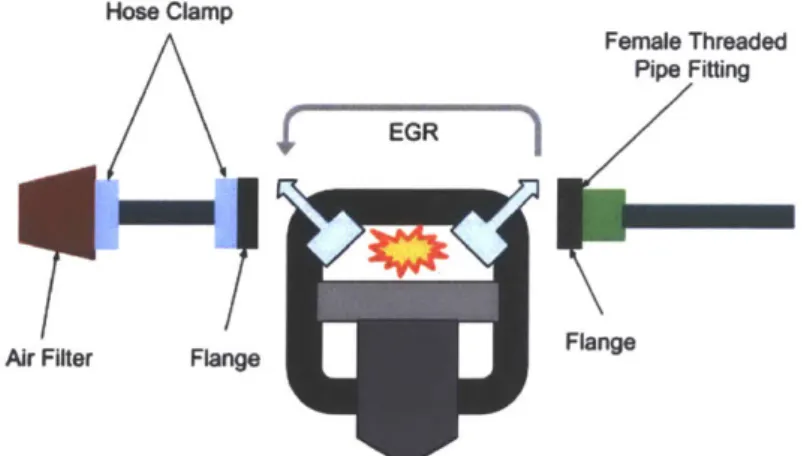
2.1 Naturally Aspirated with No After Treatment

The diagram of the naturally aspirated system with no after treatment setup is shown in Figure 2.4. Taking data using this setup is important to provide a baseline as to what would be happening without the after treatments. It helps recognize how the after treatments actually affect emissions.

Hose Clamp

Female Threaded Pipe Fitting

A

EGRI L

Ar Filter Flange Flange

Figure 2.4. Diagram of the naturally aspirated setup to run baseline tests.

With this setup, tests will be run to determine the back pressure and emissions at various speeds and loads. A sweep of loads will be run to create an engine output power from zero to nine horsepower. Speeds will range from 1500 to 3500 rpm. The results will be shown in Section

3.

2.2 Diesel Oxidation Catalyst

The DOC test setup is shown in Figure 2.5. This setup is a naturally aspirated system, so there is no turbocharger present. On the intake side, there is an air filter connected to the intake port. On the exhaust side, the gas goes through the DOC and into the emissions sensor. This and the dynamometer will be able to determine the back pressure that is present, as well as the emissions.

(22)

Hose Clamp Air Filter Female Threaded Pipe Fitting EGR FlneDiesel Oxida FM : Frng AtAjyst tion ang.

Figure 2.5. Diagram of the diesel oxidation catalyst test setup.

With this setup, tests will be run to determine the back pressure and emissions at various

speeds and loads. A sweep of loads will be run to create an engine output power from zero to nine horsepower. Speeds will range from 1500 to 3500 rpm. The results will be shown in Section

3.

2.3 Diesel Particulate Filter

The DPF test setup is shown in Figure 2.6. This setup is a naturally aspirated system, so there is no turbocharger present. On the intake side, there is an air filter connected to the intake port. On the exhaust side, the gas goes through the DPF and into the emissions sensor. This and the dynamometer will be able to determine the back pressure that is present, as well as the emissions.

Hose Clamp

Air Filter FMange

Female Threaded Pipe Fitting

EGFR

Diesel Flange P __ _ilter

Figure 2.6. Diagram of the diesel particulate filter test setup.

With this setup, tests will be run to determine the back pressure and emissions at various speeds and loads. A sweep of loads will be run to create an engine output power from zero to nine horsepower. Speeds will range from 1500 to 3500 rpm. The results will be shown in Section

3.

(23)

3. Results

3.1 Back Pressure Data

3.1.1 Back Pressure as a Function of Power and Speed

The back pressure data was determined by measuring the pressure at the engine exhaust for the system with no after treatment. For the other two systems, it was determined by measuring the pressure at both ends of the after treatment, and subtracting the inlet pressure from the outlet pressure. The data for the system with no after treatments is shown in Figure 2.7, and is shown as a function of engine power and speed. Figure 2.7 shows that for the first system, back pressure increases as engine power decreases. The data also shows that at mid-range values for engine speed, the back pressure decreases.

10 9-5 a. 1800 2000 2200 2400 2600 2800 3000 3200 3400 Speed [RPM] 0.5 0.4 0.3 0.2 0.1 0 0

Figure 2.7. Back pressure baseline data as a function of engine power and speed for the system with no after treatments.

The back pressure data for the system with the DOC is shown in Figure 2.8. This data shows that with a DOC in place, the back pressure remains consistently high for the full range of engine power and speed. Compared to the baseline data, this after treatment adds a lot of back pressure, which will lead to power loss.

(24)

7 75 51 4-3H 2 1800 2000 2200 2400 2600 2800 3000 3200 3400 Speed [RPM] 0.5 0.4 0.32 0,2 0.1 0

Figure 2.8. Back pressure data as a function of engine power and speed for a system containing a DOC.

The back pressure data for the system with the DPF is shown in Figure 2.9. This data

shows that as engine power decreases, the back pressure increases. It also shows that as engine speed decreases, back pressure increases. This is a similar trend as seen in the baseline data, but it is magnified because of the after treatment.

a.

I

8 7 1 6 5 4 3 2 0.5 0.4 0.3 0.2 0.1 0 1800 2000 2200 2400 2600 2800 3000 3200 3400 Speed [RPM]

Figure 2.9. Back pressure as a function of engine power and speed for a system with a DPF.

(25)

3.1.2 Back Pressure as a Function of Temperature and Speed

Back pressure can also be affected by the exhaust temperature. In the figures below, the data is plotted as a function of exhaust temperature and engine speed. Figure 2.10 displays the baseline data in this form. It shows that as temperature decreases, the amount of back pressure increases. It displays a similar speed trend as that shown in Figure 2.7.

700 1 7_F 550 - 0500.- 2450-a E 400-350 1800 2000 2200 2400 2600 2800 3000 3200 3400 Speed [RPM] 0.5 0.4 0.3 0.2 0.1 0

Figure 2.10. Back pressure as a function of exhaust temperature and system with no after treatments.

engine speed for a

The back pressure data for the system with the DOC is shown in Figure 2.11. The data is much higher than the baseline data, and remains this high consistently for the full range of exhaust temperatures and engine speeds.

.dm

650-

600-

(26)

-fUU 650- -0.5 600-550 - 0.4 0D500 . 2450 E 400 -0).1 350 0. 300-1800 2000 2200 2400 2600 2800 3000 3200 3400 Speed [RPM]

Figure 2.11. Back pressure as a function of exhaust temperature and engine speed for a system with a DOC.

The back pressure data for the system with the DPF is shown in Figure 2.12. This shows that as temperature decreases, back pressure increases. It also shows that back pressure is fairly independent of engine speed.

700 650 0.5 600 550 0.4 ()500. 0.3 450 E 400 0 F-350 -300 - 2501-200' L 1800 2000 2200 2400 2600 2800 3000 3200 3400 Speed [RPM)

Figure 2.12. Back pressure as a function of exhaust temperature and engine speed for a system with a DPF.

(27)

3.1.3 Back Pressure as a Function of Independent Components

The plots below shows the back pressure data for all three scenarios as a function of one component: engine power, engine speed, or exhaust temperature. This was done in order to determine which factor creates an increase in back pressure. Figure 2.13 shows the data as a function of engine power. It shows that no after treatment consistently exhibits a lower back pressure throughout the sweep of engine loads. It also shows that with no after treatment, there is a slight negative relationship between back pressure and engine power. For the system with the

DOC, back pressure remains constant throughout the sweep. For the system with the DPF, there

is a more drastic negative relationship between back pressure and engine power.

0.6 h I

* ~ None

DOC

0.5 ... ~ *. DPF FI

0.5e _{None Beat Fit}

-DOC Bs FI - *-DPF Best Fit 0.4 0.3-090 0.2-. -0.1 465 -0.2 too 0 1 2 3 4 5 6 7 8 9 10 Power [HP]

Figure 2.13. Back pressure as a function of engine power for all three scenarios. The back pressure data plotted against engine speed is shown in Figure 2.14. For the scenario with no after treatment, there is not a clear relationship between engine speed and back pressure. For the scenario with a DOC, there is no change in back pressure as engine speed varies. For the scenario with a DPF, there is a negative relationship between back pressure and engine speed, but this doesn't fit a linear model too well.

(28)

0.6 J j j ~ ________-+ None DPF None Best -DOC Beat -OPF Best r-*~ ?4 * 4

-i

1800 2000 2200 2400 2600 Speed [rpm] 2800 3000 3200 3400 3600

Figure 2.14. Back pressure as a function of engine speed for all three scenarios. The back pressure data as a function of exhaust temperature is shown in Figure 2.15. In the scenario with no after treatment, there is a negative relationship between back pressure and exhaust temperature, but the linear fit does not describe the data too well. For the system with a

DOC, back pressure is independent of exhaust temperature. For the system with a DPF, there is a

negative linear relationship between exhaust temperature and back pressure.

.- Nor Best Fit

-DOC Bet Fi

--DPF BWs Fit

200 250 300 350 400 450 Temperature [deg F1

500 550 600 650 700

Figure 2.15. Back pressure as a function of exhaust temperature for all three scenarios.

0.5[ 0.4 0.3- 0.2- a-10.1 00.1 -Ft Fit -0.2' 16C 0.6 0.3 0.2 120.1 0 -0.1 r 0 0.6 0.5

(29)

0.4-3.2 Emissions Data 3.2.1 CO Data

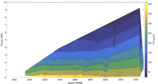
3.2.1.1 CO as a Function of Power and Speed CO emissions are shown

shows the data for the scenario decreases, the concentration of independent of engine speed.

10 9 8 7 6 5 4 3 2

below as a function of engine power and speed. Figure 2.16 with no after treatments. This demonstrates that as power

CO emissions increases. It also shows that emissions are

01 1800 2000 2200 2400 Spe Figure 2.16. CO 400 350 300 250 2008 150 100 50 2600 2800 3000 3200 3400 ed [RPM]

emissions as a function of engine power and speed for a system with no

after treatments.

The CO emissions data for the scenario with a DOC is shown in Figure 2.17. This plot demonstrates that as engine power decreases, the amount of CO emissions increases. It also shows that emissions are independent of speed for lower speeds. As speed increases, there is a negative relationship between CO emissions and engine speed. For high engine loads, the amount of CO decreases from that seen in the first situation. However, as power decreases, the amount of emissions starts to match that found in the baseline tests.

(30)

lu I400 9 350 8 7 6 ₂₅₀ 5 200 4-150 3- 2-50 0 1800 2000 2200 2400 2600 2800 3000 3200 3400 Speed [RPM]

Figure 2.17. CO emissions as a function of engine power and speed for a system with a

DOC.

The CO emissions data for the scenario with a DPF is shown in Figure 2.18. It shows that as power decreases, emissions increase. It also shows that emissions are independent of speed. The trend is similar to that seen in the baseline data, but the overall amount of CO is decreased at every step. 10400 9--350 8- 4-3 150 22008 115-1800 2000 2200 2400 2600 2800 3000 3200 3400 Speed [RPM]

Figure 2.18. CO emissions as a function of engine power and speed for a system with a DPF.

(31)

3.2.1.2 CO as a Function of Temperature and Speed

The CO emissions data as a function of temperature and speed is shown below. Figure

2.19 shows the baseline data. It shows that as exhaust temperature decreases, the amount of CO

emissions increases. It also shows a slightly negative relationship between engine speed and CO emissions. 650_r 600 F 400 350 550 S500-- ,2450-0) 9400 350 300 F 250 200 1800 2000 2200 2400 2600 Speed [RPM] I -~ 2800 3000 3200 3400 300 250 2008o 150 100 50

emissions as a function of exhaust temperature and engine speed for a system with no after treatments.

The CO emissions data for the scenario with a DOC is shown in Figure 2.20. It shows that as temperature decreases, emissions increase. This is similar to the baseline data. However, the emissions level at similar temperatures and speeds to that of the baseline is significantly less.

Figure 2.19. CO

(32)

650 600 550 a 500 450 0 E 4oo 350 300 250 200 2800 3000 3200 3400 400 350 300 250 200 0 150 100 50

The CO emissions data for the scenario with a DPF is shown in Figure 2.21. This shows a similar trend as the baseline data, with a negative relationship between temperature and emissions. However, it shows a slightly more negative relationship between speed and emissions levels. It causes a general decrease in emissions levels, but not as much as the DOC.

1800 2000 2200 2400 2600 Speed [RPM] 400 350 300 250 2000 150 100 so 2800 3000 3200 3400

Figure 2.21. CO emissions as a function of exhaust temperature and engine system with a DPF.

1800 2000 2200 2400 2600

Speed [RPM

Figure 2.20. CO emissions as a function of exhaust temperature and engine speed or a system with a DOC.

7007 650 600 K 550 CM500 .2450 4) CL 400 350 300 250-200' speed for a -j fill] -.. -

(33)

0-3.2.1.3 CO as a Function of Independent Components

The CO emissions data is shown as a function of engine power for all three scenarios in Figure 2.22. This demonstrates that there is a similar relationship for all three scenarios. It shows a negative relationship between engine power and CO emissions level that stabilizes to a single value at high power. The DOC decreases emissions at high power the most, while the DPF decreases emissions at high power slightly.

Non DO0C -*-DPF 8 B Best Fit C Best Fit Best Fit 6 7 8 9 10

Figure 2.22. CO as a function of engine power for all three scenarios.

The CO emissions data as a function of engine speed is shown in Figure 2.23. This data suggests that there is not a relationship between speed and emissions level.

450 400 300 250 0 8 200 150 -100 50-OL 0 3 4 w2 5 Power [HP] i

(34)

WM

1800 2000 2200 2400 2600

Speed (rpm]

2800 3000 3200 3400 3600

Figure 2.23. CO as a function of engine speed for all three scenarios.

The CO emissions data as a function of exhaust temperature is shown in Figure 2.24. There is a similar negative relationship between exhaust temperature and emissions level. It shows similar emissions levels for baseline data and with the DPF. The DOC significantly decreases CO emissions at higher temperatures.

400 350 300 h 250 0. 8 2001 150-100

F

250 300 350 400 450 Temperature [deg F] 500 550 600 650 700

Figure 2.24. CO as a function of exhaust temperature for all three scenarios. 400

350-300

k

-250 F . 01 o 200[ 150-100F 50-01 1600 .None . Doc *DPF SNone Best F --DC Best F -- DPF BOSt F *~ 0-200 -A *None .DOC DPF None BeMFit -DOC Best Fk -DPF Bet Fit 'd IL Arn It k

(35)

-Ad

3.2.2 C02 Data

3.2.2.1 C02 as a Function of Power and Speed

The C02 emissions data as a function of engine power and speed is shown below. The baseline data is shown in Figure 2.25. This data demonstrates that as engine power increases,

C02 emissions also increase. There is no relationship between engine speed and emissions. 10! 9 8 5 4- 2-0 1800 2000 2200 2400 2600 2800 3000 3200 3400 Speed [RPM]

Figure 2.25. C02 as a function of engine power and speed or the system with no after treatments.

The C02 emissions data as a function of engine speed and power for the system with a

DOC is shown in Figure 2.26. It shows a similar trend as that seen in the baseline data. However,

it shows a general decrease in C02 at the various engine loads.

5 4.5 4 ('4 0 C-) 3.5 3 2.5 2 1.5

(36)

10 --- 15 9 4.5 80 0. ~3. 4ale 2. 2H 2 01 1800 2000 2200 2400 2600 2800 3000 3200 3400 Speed [RPM]

Figure 2.26. C02 as a function of engine power and speed for the system with a DOC.

The C02 emissions data as a function of engine speed and power for the system with a DPF is shown in Figure 2.27. This exhibits a similar trend as shown in the baseline data. However, there is a general decrease in C02 emissions at the various engine loads.

10 9 .5 82 1.5 8 -(L 3 4-3- 2.5 2 -2 1 1800 2000 2200 2400 2600 2800 3000 3200 3400 Speed [RPM]

Figure 2.27. C02 as a function of engine power and speed for the system with a DPF. 3.2.2.2 C02 as a Function of Temperature and Speed

The C02 emissions data as a function of exhaust temperature and engine speed is shown below. The baseline data is shown in Figure 2.28. As temperature increases, the amount of C02

(37)

emissions also increases. There is also a slightly negative relationship between engine speed and emissions level. 700 - 650- 60-550 0500 .3450 0. E 400 350 300 - 250-1800 2000 2200 Figure 2.28. C02 as a function 2400 2600 Speed (RPM] 2800 3000 3200 3400 5 4.5 4 3.5 3 2.5 U. 2 1.5

of exhaust temperature and engine speed for the system with no after treatments.

The C02 emissions data as a function of exhaust temperature and engine speed for the system with a DOC is shown in Figure 2.29. There is a similar trend as that shown in the baseline data. However, there is a general decrease in C02 emissions at the varying levels of speed and temperature.

-. A 5 4.5 4 3.5 C'4 0 C.) 3 2.5 2

1

700 650

L

600 - 550-500h S 450 9400 350 - 300-250 -4

(38)

The C02 emissions data as a function of exhaust temperature and engine speed for the system with a DPF is shown in Figure 2.30. The trends are similar to those seen in the baseline data. There is also a general decrease in the C02 emissions at the varying temperature and speed levels. 700-650 600 ~ 550 500 450 E 400- I-350 300-250 A 1800 2000 2200 2400 2600 2800 3000 3200 3400 Speed [RPM]

Figure 2.30. C02 as a function of exhaust temperature with a DPF.

and engine speed for the system

3.2.2.3 C02 as a Function of Independent Components

The C02 emissions data as a function of engine power for all three scenarios is shown in Figure 2.31. This data shows that as power increases, C02 emissions increase. This trend remains the same for all three scenarios.

I-F 5 4.5 4 3.5 3 2.5 2 1.5

1

(39)

0D

0 1 2 3 4 5

Power (HPI

6 7 8 9 10

Figure 2.31. C02 as a function of engine power for all three scenarios.

The C02 emissions data three scenarios. This data shows

C02 emissions concentration. 5 4.5 I-4 ~3.5 0 803 2.5- 2- 1.5-1600

as a function of engine speed is shown in Figure 2.32 for all that there is no distinct relationship between engine speed and

* None

.Doc

DPF

None Best Fit

-DOC Beet Fit

-DPF Bet Fit -G. -I I I I I 2800 3000 3200 3400 3600

Figure 2.32. C02 as a function of engine speed for all three scenarios.

The C02 emissions data as a function of exhaust temperature for all three scenarios is 5 4.51 4 03.5 2.5 1800 2000 2200 2400 2600 Speed [rpm] SNone B i

.. + -DOC Best Fit

F -DPF Beat Fit

-0*

- **

.Ot. . .4,

(40)

5.5 I

.Nori

5 DPF

None Best Fit

--- OC Best Fkt 4.5 - -DPF Bmst Fit-4 :F3.5-0 - 3 2.5-2 200 250 300 350 400 450 500 550 600 650 700 Temperature [deg F]

Figure 2.33. C02 as a function of exhaust temperature for all three scenarios.

3.2.3 HC Data

3.2.3.1 HC as a Function of Power and Speed

The HC emissions as a function of engine power and speed are shown below. The baseline data is shown in Figure 2.34. It shows that as engine power increases, the amount of HC also increases. There is no relationship between emissions level and engine speed.

10 T 540

9

520 8 5W0 B9--7480 480 66 440 420 4 -2 360 1V 340 320 1800 2000 2200 2400 2600 2800 3000 3200 3400 Speed [RPM)

Figure 2.34. HC as a function of engine power and speed for the system with no after treatments.

(41)

The HC emissions data as a function of engine power and speed for the system with a

DOC is shown in Figure 2.35. It shows that as engine power increases, emissions levels increase,

which is a similar trend as that seen in the baseline data. It also shows no clear relationship between emissions level and engine speed. For low power applications, the DOC actually produces more emissions than the baseline setup does. As the engine moves into higher power applications, the DOC begins to decrease emissions levels.

8 6 -5 4 1 2 3- 2-01 1800 2000 -- 1 2200 2400 2600 Speed [RPM] 2800 3000 3200 3400

Figure 2.35. HC as a function of engine power and speed for the system with a DOC. The HC emissions data as a function of engine power and speed for the system with a DPF is shown in Figure 2.36. This figure shows a similar trend with respect to power and speed as that seen in the baseline test. However, it shows a decrease in HC emissions at higher engine loads, and an increase in HC emissions at lower engine loads.

10 r 9g 0 a. 540 520 500 480 460 440 420 Q 400 380 360 340 320

(42)

10of 9K 0 a. 2000 2200 2400 2600 2800 3000 3200 3400 Speed [RPM]

Figure 2.36. HC as a function of engine power and speed for the system with a DPF. 3.2.3.2 HC as a Function of Temperature and Speed

The HC emissions data as a function of exhaust temperature and speed is shown below. The baseline data is shown in Figure 2.37. This data shows that as exhaust temperatures increase,

HC emissions increase. There is no clear relationship between emissions and speed.

2200 2400 2600 2800 3000 3200 3400

Speed [RPM]

Figure 2.37. HC as a function of exhaust temperature and engine speed for the system with no after treatments.

The HC emissions data as a function of exhaust temperature and engine speed for the system with a DOC is shown in Figure 2.38. This data shows similar temperature and speed

540 520 500 480 460 440_w C. 420 0) 400 380 360 340 320 0' 1800 700 650 540 520 600 550 5001 450 (D E 400 K 350 300 250 2001 -4 I 1800 2000 480 420 440 420 L) 400 380 360 340 320

7'7"'7

I I I I I

(43)

trends as that seen in the baseline test. However at low temperatures, it shows an increase in HC emissions. As the temperature increases, the HC emissions begin to decrease.

700 - 540 650- - 520 500 600-480 550- . 4 460 0500 440' 0 .C 450. 4200u ~~400 350- 8 300- 6 25034 200 320 1800 2000 2200 2400 2600 2800 3000 3200 3400 Speed [RPM]

Figure 2.38. HC as a function of exhaust temperature and engine speed for the system with a DOC.

The HC emissions data as a function of exhaust temperature and engine speed for the system with a DPF is shown in Figure 2.39. This data shows trends that are similar to those of the baseline data for exhaust temperature. For engine speed, it starts to show a negative relationship between speed and emissions level. For low temperatures, there is an increase in HC emissions when compared to the baseline data. At high temperatures, the HC emissions decrease with respect to the baseline data.

(44)

2200 2400 2600

Speed [RPM]

Figure 2.39. HC as a function of exhaust temperature and a DPF.

engine speed for the system with

3.2.3.3 HC as a Function of Independent Components

The HC emissions data as a function of engine power for all three scenarios is shown in Figure 2.40. This data shows a positive relationship between emissions and engine power. For low engine powers, the system with the DOC produces more HC than the baseline system. At around 4 HP, the DOC begins to produce less HC emissions. The DPF produces less HC emissions than the natural system at all engine loads above 1 HP. At low power, the DPF produces more HC emissions.

550 500 450 400 350 0 1 2 3 4 5 Power [HP] 6 7 8 9 10

Figure 2.40. HC as a function of engine power for all three scenarios.

700 r 650 600 550 M500 450 E 400 350 320 250 540 520 500 480 460 440 420o 400 380 360 340 320 1800 2000 2800 3000 3200 3400 SNonke so# DPF 7# so - B* 00* I I I I

(45)

The HC emissions data as a function of engine speed for all three systems is shown in Figure 2.41. The data shows no trend between engine speed and emissions level.

None IIDPF b Nor* Best Fd -DOC Best Fkt 0 -DPF Best Fit 1600 1800 2000 2200 2400 2600 Speed [rpm] 2800 3000 3200 3400 3600

Figure 2.41. HC as a function of engine speed for all three scenarios.

The HC emissions data as a function of exhaust temperature for all three scenarios is shown in Figure 2.42. This shows a positive relationship between exhaust temperature and emissions level. For low temperatures, the DOC produces more HC emissions than the natural system. At around 325 degrees F, the DOC begins to produce less HC emissions. The DPF produces less HC emissions at all temperatures.

500 450 E 400 350 F500 -450 T 400 350t-0 . DOC o DPF Name Best Ft IDOC BWs Fkt ft IDPF Besti 550I

(46)

3.2.4 NO Data

3.2.4.1 NO as a Function of Power and Speed The NO emissions data as a function baseline data is shown in Figure 2.43. This emissions levels also increase. It also shows emissions levels. 101 7'-I 0 0 0. 5 4k 3b 2-1k

of engine power and speed is shown below. The data shows that as engine power increases, NO a negative relationship between engine speed and

400 350 300 250 R 150 100 1800 2000 2200 2400 2600 2800 3000 3200 3400 Speed [RPM)

Figure 2.43. NO as a function of engine power and speed for the system with no after treatments.

The NO emissions data as a function of engine speed and power for the system with a

DOC is shown in Figure 2.44. This data shows a more negative relationship between engine

speed and emissions level. It also shows that as engine power increase, so does NO emissions. For lower power levels, the amount of NO emissions is greater than the baseline level. As power increases, the emissions levels begin to be less than those shown in the baseline data.

(47)

goo 2 8 -6 aj5 3h 2 0 -1800 2000 2200 2400 2600 2800 3000 3200 3400 Speed [RPM]

Figure 2.44. NO as a function of engine power and speed for the with a DOC.

The NO emissions data as a function of engine power and speed for the system with a DPF is shown in Figure 2.45. This data shows similar trends for engine speed and power as those seen in the baseline data. However, at lower engine loads, there is a general increase in NO emissions. As the engine power increases, the emissions level begins to decrease.

10 9 -7 6 5 5r 4 3 1800 2000 2200 2400 2600 Speed [RPM] 2800 3000 3200 3400