HAL Id: hal-00799235
https://hal-enpc.archives-ouvertes.fr/hal-00799235
Submitted on 11 Mar 2013
HAL is a multi-disciplinary open access archive for the deposit and dissemination of sci-entific research documents, whether they are pub-lished or not. The documents may come from teaching and research institutions in France or abroad, or from public or private research centers.
L’archive ouverte pluridisciplinaire HAL, est destinée au dépôt et à la diffusion de documents scientifiques de niveau recherche, publiés ou non, émanant des établissements d’enseignement et de recherche français ou étrangers, des laboratoires publics ou privés.
F. Grazi, H. Waisman
To cite this version:
F. Grazi, H. Waisman. Urban Agglomeration Economies in Climate Policy : A Dynamic CGE Ap-proach. 2009. �hal-00799235�
DOCUMENTS DE TRAVAIL / WORKING PAPERS
No 17-2009
Urban Agglomeration Economies in Climate
Policy: A Dynamic CGE Approach
Fabio Grazi
Henri Waisman
November 2009
C.I.R.E.D.
Centre International de Recherches sur l'Environnement et le Développement
UMR
8568
CNRS
/
EHESS
/
ENPC
/
ENGREF
/
CIRAD /
M
ÉTÉOF
RANCE45 bis, avenue de la Belle Gabrielle
F-94736 Nogent sur Marne CEDEX
Tel : (33) 1 43 94 73 73 / Fax : (33) 1 43 94 73 70
www.centre-cired.fr
ABSTRACT
This paper designs and solves a theoretical model in the light of the new economic geography to assess the role of urban land use in driving local energy consumption pathways that affect global climate change. To inform on the urban economic sectors of climate pressure we offer new modeling arguments and take the next step of testing them in simulations using computable general equilibrium (CGE) model for international climate policy. The exercise of embedding urban economies in a CGE framework is operationalized on the U.S. context. Both the modeling arguments and the simulations indicate that setting spatial policies for the control of long-run density patterns of cities is beneficial strategy to curtail national dependence on energy imports. When faced with international climate agreement that sets targets on carbon emissions, the national government may resort to urban infrastructure policies to offset the cost of an exogenous carbon tax (JEL C68, Q54, R12).
Keywords: CO₂ emissions, Energy use, Infrastructure investments, Urban and regional economics
RÉSUMÉ
Ce papier décrit et résout un model théorique fondé sur les principes de la nouvelle économie géographique et permettant d’évaluer le rôle de l’espace urbain comme déterminant des trajectoires de consommation d’énergie locale affectant le changement climatique global. Afin de mieux informer sur les secteurs de l’économie urbaine à considérer dans le cadre du changement climatique, nous proposons un cadre de modélisation innovant, testé numériquement au travers de simulations utilisant un model d’équilibre général calculable construit pour l’évaluation des politiques climatiques internationales. L’intégration des économies urbaines au sein d’une telle architecture est effectuée pour les USA. Aussi bien les principes de modélisation que les résultats numériques des simulations démontrent que la mise en place de politiques d’infrastructure pour le contrôle du développement de long-terme des villes est une stratégie bénéfique pour réduire la dépendance nationale vis-à-vis des importations d’énergie. Dans un contexte d’accord climatique international imposant des objectifs de réduction d’émissions de carbone, les gouvernements nationaux pourraient avoir recours à des politiques d’infrastructure au niveau urbain pour diminuer le coût de l’imposition d’une taxe carbone (JEL C68, Q54, R12).
Mots-clés : Emissions de CO₂, Consommation d’énergie, Investissements sur les infrastructures,
Economie urbaine et régionale
Approach
Fabio GRAZIy and Henri WAISMAN
International Research Centre on the Environment and Development (CIRED, umr ENPC/ParisTech & EHESS/CNRS), Paris, France.
I
Introduction
There is an increasing attention in climate policy literature towards the ne-cessity of investigating the dynamics of the impacts of economic activities where they speci…cally arise (e.g., IPCC, 2001; Tietenberg, 2003; OECD, 2006; Grazi et al., 2008). Urbanization, city growth, and economic develop-ment are strictly related phenomena that have many important implications on global environmental change. First, urban dynamics and climate change are related through emissions and energy consumption from economic ac-tivities located in cities. Second, spatial organization and its counterpart transport in‡uence the extent of global warming, especially through reduced commuting distances from private automobiles and consequently lower carbon emissions. A serious search for sustainable systems requires therefore analysis of spatial patterns. Modeling regional/urban climate change is a logical next step of climate change research.
To study the relationship between spatial patterns at the urban and re-gional scale and climate (un)sustainability in a way that is consistent with mi-croeconomic theory, we build up a model that can be incorporated in a Com-putable General Equilibrium modeling framework for climate policy analysis. In particular, we focus on how dynamic recursive modeling frameworks for the study of climate policy options capture the spatial dimension of an econ-omy and the impacts of urban activities on climate. In analyzing where an economy chooses to locate and under what determinants it distributes across
We are indebted to John Reilly for helpful discussions during the preparation of this article. We thank Jean-Charles Hourcade, Olivier Sassi and seminar audience at CIRED, Paris and MIT-EPPA, Cambridge MA for useful comments. This article has been …rst conceived while Fabio Grazi was visiting the Joint Program on the Science and Policy of Global Change at MIT. He gratefully acknowledges the institution for hospitality. The usual disclaimer applies.
yAuthor for correspondence. Mail : 45bis avenue de la Belle Gabrielle, 94736 Nogent sur
the space our model draws upon the new economic geography (NEG), but modi…es it, as it is made clear further below. Since its appearance, due to the work of Krugman (1991), NEG has brought up interesting contributions to the understanding of those patterns along which an economy locates. Com-prehension of the spatial determinants of regional economic development is set at the core issue of NEG’s investigation, which particularly looks at how …rms (and consequently households) agglomerate or sprawl. The NEG ap-proach employs a two-region, two-sector general equilibrium framework and makes use of a set of assumptions that combine monopolistic competition à la Dixit and Stiglitz (1977) and ‘iceberg’trade costs à la Samuelson (1952) in a mathematically tractable manner.
In the present paper, a simple model is proposed that allows for regional economies where multiple urban agglomerations dynamically evolve and al-ternative con…gurations of city growth potentially emerge. In so doing, we need to slightly reformulate the theory described above. Indeed the NEG theory posits that manufacturing-like …rms end up agglomerating in certain places (cities) may be true to some extent, but it is certainly not complete. Here we aim to show not only what optimal agglomeration (city) size arises from …rms’ location choice, but also determine under what conditions …rms choose to locate in a wide, more realistic range of alternative agglomerations (cities). This suggests that a value of agglomeration may exist for fairly di¤er-ent industry types. To the best of our knowledge, this spatial ‘disaggregation’ of the …rms’location preferences over multiple (endogenous) agglomerations is simply not available in the NEG framework. Yet, this is clearly what we observe in the real world. In order to render a realistic picture of spatial dis-tribution patterns of an economy, we therefore consider households enjoying identical welfare levels except that they face some external bene…ts and costs that are both function of how close to the city-center their location prefer-ence falls. Similarly, we assume that all …rms have identical …xed production costs structures but face di¤erent variable costs in that they internalize the workers’external bene…ts and costs through the wage rate. In line with the NEG theory, our approach distinguishes as external bene…ts the economies of scale that arise from economic agents (both …rms and workers/households) being located close together (e.g., facilitation of interchange among …rms, job ‡exibility, ability to support social and cultural events). On the other hand, external costs are re‡ected in the diseconomies that arise from congestion (e.g., increased land costs and higher commuting costs for workers, and larger salaries that the …rms have to pay to compensate workers for the costs of living in urban areas).
In addition to allowing for spatial disaggregation of the production sec-tor, our model introduces other signi…cant features that make it diverge from the standard NEG framework. Dynamics is enabled through migration de-cisions of …rms, whose location preferences go towards those agglomeration markets that o¤er the best investment opportunities. This is not the case in the standard NEG framework, in which dynamics is typically modeled
through interregional mobility of workers responding to utility maximization. This in turn introduces a conceptual innovation of our model that better …ts the modern structure of the production sector, where decisions are taken as a result of trade-o¤s between …rms’pro…ts and managers’and shareholders’ interests. Finally, we explain agglomeration spillover e¤ects endogenously, in a less stylized, more realistic analytical framework. By breaking the duality of the production sector (two-region, two sectors, two factors of production) through the introduction of a third input factor of production (intermedi-ate consumtpion), we model the bene…ts from reduced (transaction) costs of intermediate goods as a result of scale economies, while still maintening the standard increasing returns structure on the production cost function of …rms. Agglomeration spillover e¤ects have been recognized in the economic litera-ture on trade theory and urban economics since Marshall and Chamberlin, but their formal representation has turned out to be di¢ cult and controversial (Ciccone, 2002).
Stylized analytical approaches typically fall short of rendering a complete picture of the complexity that animates sustainability debate, especially in the …eld of climate change, where CO2(major responsible for global warming)
and other green house gas (GHG) emissions represent a global transboundary threat that can hardly be incorporated in a simpli…ed analytical framework. Moreover, policy actions require long-run forecasting of complex dynamic sys-tems a¤ecting climate, as the whole economy. For these reasons, numerical analysis techniques like computable general equilibrium (CGE) models are seen as more reliable guides to address the relationship between determinants of economic development and forces inducing climatic variations (Böhringer and Löschel, 2006). Our NEG model of urban economies is developed to be integrated by CIRED Impact Assessment of Climate Policies (Imaclim-R, hereafter) (Crassous et al., 2006), a global CGE model of economic growth, international trade, and CO2 (carbon) emissions. Modular integration with
Imaclim-R enables capturing the global environmental impacts stemming from all activities associated with urban land use and translate these through negative externalities into welfare e¤ects. Imaclim-R model has been applied to a number of international policy studies and it is recognized as an innovative analytical tool for policy scenario analysis. Two are the points of innovations that characterize Imaclim-R with respect to other reknown CGE models in use to climate policy: i) the transition costs between two steady-state equilib-ria are endogenously generated by the interplay between non-perfect foresight and the inertia of technical systems ii) the physical technical coe¢ cients al-low for a transparent incorporation of bottom-up information and ‘routine’ behaviors as drivers of technical change. These modeling features are particu-larly well suited to analyze the complexity of urban phenomena as they allow capturing the uncertainty related to agents’ spatial behavior when multiple locations are available. Like other recursive frameworks (Paltsev et al., 2004), the dynamics in Imaclim-R accounts for imperfect expectations of economic agents when taking decisions over equipment, technology, location.
The remainder of this paper is organized as follows. Section II provides a brief discussion on CIRED/Imaclim-R model, the CGE modeling framework used for this study. Section III presents the static model, as well as the dy-namic setting to be embedded in Imaclim-R. Section IV presents our results. Section V …nally concludes.
II
The IMACLIM-R CGE modeling framework
CGE models are being increasingly used by research institutes and interna-tional organizations as well, as numerical instruments that are capable of pro-viding policy makers with a wide range of information on the several economic sectors of climate pressure. Standard CGE models adopted in environmental economic analyses base on multi-regional, multi-sectoral analytical framework accounting for economy’s e¢ ciency and distributional e¤ects of policy mea-sures (mainly, carbon taxes/subsidies and emission trading permits) aimed at CO2 abatement. They can in fact provide numerical outcomes under di¤erent
policy scenarios, simulating what economic impacts arise from speci…c policy interventions. In consequence of the cost (bene…t) pressure exercised on its sectors by a tax (subsidy), the world economy reacts adjusting production and consumption, as well as reallocating input factors according to pre…xed factors of substitutability.
Most empirical CGE models are static models, mostly because a static framework allows for accounting of policy interferences, using counterfactual simulations on a calibrated equilibrium to investigate the e¤ect of price mea-sures of new introduction. However, a dynamic framework is essential in models that aim at accomplishing the twofold task of accounting for policy interference on economic welfare and forecasting carbon emissions from eco-nomic activities. Indeed, taking into account the dynamic dimension allows capturing the change in (both human and physical) capital stock as a conse-quence of some exogenous policy pattern, as well as addressing the issues of resource allocation over time, economic growth, environmental degradation.
The Imaclim-R model used in this study is a dynamic recursive model in that savings and investments a¤ect the capital stock as function of in-come only in the current period (Crassous et al., 2006).1 It is based on an explicit representation of the economy both in money metric values and physi-cal quantities linked by a price vector. This dual vision of the economy, which comes back to the Arrow-Debreu theoretical framework, guarantees that the projected economy is supported by a realistic technical background and, con-versely, that any projected technical system corresponds to realistic economic ‡ows and consistent set of relative prices.
Calibration data rely upon the combination of GTAP dataset and explicit energy balances, the former providing detailed accounts of regional
produc-1This is opposed to what occurs in forward-looking intertemporal optimization
tion, consumption and international trade, and the latter giving a complete picture of patterns of energy production and consumption. The base year used for policy scenario analysis is the 2001, and the model covers the pe-riod 2001-2100, in one year steps. The version of the Imaclim-R model used in this paper divides the world economy into 12 regions and 12 sectors for which details are reported in Table 1. Two transport modes auto-produced by households (personal vehicles, and non-motorized transportation) are also included.
Table 1:
Key dimensions of the IMACLIM-R model
Region
USA Canada Europe
OECD Paci…c (JP, AU, NZ, KR) Former Soviet Union
China India Brazil Middle-East Countries Africa Rest of Asia
Rest of Latin America
Sector Energy Primary Energy Coal Oil Gas
Transformed Energy Liquid Fuels
Electricity Transport Air Water Others Goods & Services Construction Agriculture Energy-intensive Industry Composite (including Services)
Note: A number of primary energy carriers are used. Concerning liquid fuels, we consider oil, biomass (biofuels) and coal (Coal-To-Liquid). As for the electricity sub-sector, we consider coal, gas, oil, hydro, nuclear and renewables.
The Imaclim-R model adopts a recursive structure that allows a system-atic exchange of information between:
and labor intensity are …xed (a Leontief production function), capital is treated as a production capacity (partially or fully exploited) and de-mand from representative households result from utility maximization under income and time-budget constraints. Solving this equilibrium at date t provides a consistent set of physical and money ‡ows linked by endogenous relative prices. As a closed model, monetary resource circu-larly ‡ow internally to the system: all the revenues from the production are either redistributed among the consumers (as returns to capital and labor) or within the production sectors (as payment for intermediate goods), or given to government (as taxes). The (passive) government is seen as a collector of taxes and re-distributor of pro…ts to the consumers. ii. Dynamic modules composed of a ‘growth engine’with endogenous tech-nical change, and sector-speci…c reduced forms of technology-rich mod-els. The latter assess the reaction of technical systems to the economic signals stemming from the static equilibrium at time t (prices, wages, pro…t margins) and send back this information to the static module in the form of new production coe¢ cients for calculating the equilibrium at time t + 1. In this putty-clay structure, technical choices can be made on the new equipment vintages every year, but do not change the coe¢ -cients of the average technology embodied in the pre-existing equipment stock.
Conventionally, the growth engine is composed of exogenous demographic trends and labor productivity changes, but constraints on investments (in a context of inertias on equipment and non-perfect expectations) lead to en-dogenous gaps between potential and real growth. This structure captures the existence of ‘transition costs’ due to non optimal responses of the economic system to random shocks around an optimal steady state (Solow, 1988).
Available domestic …nancial resources for investment are given by the sum of savings and the share of returns to capital that is directly re-invested. Since we assume that households’savings are mostly linked to the dynamics of regional population, we set saving rates exogenously, as demographic trends. A share of available investments is traded internationally, and resulting net available …nancial resources are distributed among sectors according to their expected needs in terms of new producing capacities.
For the majority of traded goods in Imaclim-R (exception being energy trade), international trade is modeled following Armington’s approach (Arm-ington, 1969) for not perfect substitute goods. Armington assumption dis-tinguishes domestically produced goods from imported commodities by the same industry on the base of the elasticity of substitution between them. The importance of Armington elasticity parameter can be seen in allowing the evaluation of economy’s response to a certain carbon cap policy set on a group of countries. Considering the production of a composite good, the increased costs of producing intensive energy goods of the composite in those
countries lead to a drop in domestic supply favoring imports from foreigner industries that are not burdened by the carbon constraint.
As noted above, the Imaclim-R model has been conceived to accomplish a twofold task: computing the carbon emissions arising from economic activities and assessing the e¤ects of emission control measures on the economy. In Imaclim-R policy measures result from economic incentives modeled through carbon taxes di¤erentiated across sectors and regions, infrastructure policy, and norms on equipment.
III
The Spatial Economy
A The static model
The world is composed of many regions each of which can be envisaged as a mass of urban agglomerations. Urban agglomeration land is conceived as monocentric, axi-symmetric city spread along one-dimensional space x 2 d, where d is the overall city size. Like traditionally approached by urban and regional economics since von Thünen (1966), the central business district (CBD), situated at the origin x = 0, is the location where …rms choose to dis-tribute once they enter the agglomeration. All economic activities take place in the j CBD, whereas the urban population is distributed within circular pe-ripheral areas surrounding it. In our economy three types of decision-makers exist: governments, producers, and consumers. We purposely abstract from all income distributional issues, and assume that the government chooses housing policies that maximize the utility of the representative consumer. Pro…t-maximizing …rms do not consume land, while utility-maximizing work-ers do. Urban workwork-ers settled at a certain point x of d consume j(x) units of
land and commute x to the CBD. The number of urban workers Lj is given
by: Lj = Z 0 jxj dj dx j(x) : (1)
At the land market equilibrium, workers are indi¤erent between any x-location around the CBD of agglomeration j 2 J. This comes down to as-suming that all people living inside each peripheral rings at each point x face identical external costs resulting from the interplay between di¤erent com-muting costs (being di¤erent the distance from each individual’s residential place and the CBD, where jobs and all varieties of the di¤erentiated goods are available) and housing costs (being heterogeneous the value and the con-sumption of land throughout the periphery).
Government owns the available land and decides of the spatial distribution of housing supply. Hence, heterogeneity of density within the agglomeration does not result from households’ preferences over the available land but is rather exogenously set. We take the trend for the density function j(x) as
given and choose a power functional form for the sake of simplicity.
j(x) = bjx ; 0 < 1:2 (2)
As in Murata and Thisse (2005), each (urban) worker supplies one unit of labor. Considering unitary commuting costs > 0 in the ‘iceberg form’à la Samuelson (1954),3 the e¤ective labor supply of a worker living in the urban area at a distance x from the CBD is:
sj(x) = 1 2 j j x j; x 2 [ dj; dj] : (3)
Condition: 0 < j 2d1j ensures positive labor supply.
The total e¤ective labor supply throughout the urban area is therefore:
Sj = Z 0 jxj dj s(x) j(x) dx = 2d 1 j bj(1 ) 1 2 j 1 2 dj ; (4)
whereas the total potential labor supply is given by:
Lj = Z 0 jxj dj 1 j(x) dx = 2d 1 j bj(1 ) (5)
Letting wj be the wage rate …rms pay to laborers to carry out their
ac-tivity within the j-urban area, commuting costs CCj faced by one worker in
agglomeration j result from the losses of e¤ective labor. Combining (4) and (5), we obtain: CCj = (Lj Sj) wj Lj = 2 j 1 2 djwj: (6)
We normalize at zero the rent value of the land located at the edges of the city: Rj(dj) = 0. Given that all urban workers are identical from a welfare
perspective, and given the wage rate wj laborers earn to work in urban area
j, using (3) the value of worker’s income j net of commuting costs 2 jxwj
and rent costs Rj(x) is the same throughout the urban city. Precisely:
j = sj(x)wj j(x)Rj(x) = sj( dj)wj = sj(dj)wj = (1 2 jdj)wj: (7)
From (7), the equilibrium land rent for an evenly distributed urban
work-2Condition 0 ensures that
j(x) is an increasing function, so that the empirical
evidence of higher population density in the centre of the city is captured. Condition < 1 is necessary to have population convergence in (1).
3Considering di¤erent unitary commuting costs
j across the agglomerations captures
ing population in region j is simply derived, as follows: Rj(x) =
2 j(dj j x j) j(x)
wj: (8)
In order to comprehend how the land rent is distributed over the urban workers by the local government, we …rst calculate the aggregated land cost by integrating Rj(x) over the distance x that represents the available urban
land, and then divide the resulting …gure by the labor force that is active in the city: RCj = Z 0 jxj dj j(x)Rj(x) dx j(x) Lj = 2 j 1 2 djwj: (9)
Combining (6) and (9) gives CCj
RCj = 1 ; which determines the distribution
of external costs between commuting and housing: the lower , the more commuting costs are relatively important. From each laborer’s income, an amount: CCj+ RCj = ECjLis deduced as compensation to live in the urban
area. This amount is expected to a¤ect consumer’s purchasing power j:
Consumption We consider a regional economy entailing a continuum of agglomerations (labeled j = (1; J )), one composite sector (the Imaclim-R industrial and service sectors) and one di¤erentiated good q. We assume that the many …rms of the industry-plus-service type composing our economy pro-duce each one variety (labeled i = (1; N )) of one type of the di¤erentiated good q under increasing returns to scale. Therefore, the number of available varieties in each agglomeration j, nj 2 N, is equal to the number of …rms that
are active in the same agglomeration. All goods can be traded internation-ally and each component of total demand is composed of both imported and domestic goods. Unlike the standard NEG literature, we avoid tracking bi-lateral ‡ows, as this would excessively complicate our model due to the many agglomerations our approach allows for. For the purpose of our simulations, all trade ‡ows are assumed to end up in an international pool (labeled h) that processes the exported varieties and re-allocates them across agglomerations. For a given fraction of the nj varieties that agglomeration j exports to the
pool h, it receives back nh varieties of the same good from the pool h, such
that: Rj=0J nj+ nhdj = N:
We de…ne a price index Pj of the composite good available in
agglomera-tion j in order to be able to treat the various products as a single group.
Pj = Z nj i=0 pjj(i)1 di + Z nh i=0 p1hj (i)di 1 1 : (10)
The economy employs a unit mass of mobile workers L: Wherever they are employed, the L laborers are both input production factors and output
end-users. Given a certain net income j based on the wage wj that a laborer
earns from working at a the j-agglomeration, she has to decide of its alloca-tion over the consumpalloca-tion of the di¤erentiated good D. We consider house-holds that reach identical welfare levels and bare identical external costs ECjL stemming from being located in the j agglomeration (see eq. (7)). Given individual’s utility Uj de…ned over the disposable income j for
consump-tion of the composite good Dj in each agglomeration j, welfare maximization
behavior imposes:
max Uj = Uj[Dj( j)] : (11)
Price and utility homogeneity throughout the j-city impose that aggre-gate consumption of the composite good is independent on the distance x from the j-core. Letting cjj(i) be the consumption of variety i produced
do-mestically and chj(i) the consumption of the variety coming from the pool h,
the constant-across-city utility from goods aggregate consumption is:
Dj= Z nj i=0 cjj(i)( 1)= di + Z nh i=0 chj(i)(" 1)= di 1 : (12)
A consumer has to satisfy the following budget constraint: Z nj i=0 pjj(i) cjj(i) di + Z nh i=0 phj(i)chj(i)di = j: (13)
Here j is the net disposable income for consumption, already discounted
from external costs for laborers ECjL (see eq. (7)).
Maximizing utility given in (12) subject to (13) gives the aggregate de-mand in region j for a variety i domestically produced and coming from the pool h; respectively: cjj(i) = Lj jpjjP(i)1 j chj(i) = Lj j phj(i) Pj1 : (14)
Production All …rms producing in a given agglomeration j incur the same production costs and rely upon the same input factors: intermediate con-sumption Zj, capital Xj, and labor lj. Capital and labor are spatially
mo-bile. Intermediate consumption is referred to as ’material’ and corresponds to the aggregate Imaclim-R sector that includes consumption of goods and transport. We consider intermediate consumption as subject to external economies of scale resulting from improved production process through some agglomeration-speci…c technology spillover, as follows:
Zj =
Z0
nj : (15)
Here nj is the given number of active …rms in region j, Z0 is a constant
captures the non linearity of the external ‘agglomeration e¤ect’ (Fujita and Thisse, 1996; Grazi et al., 2007).
Due to the …xed input requirement , the amount of productive capital in agglomeration j, Xj, is proportional to the number of domestic …rms, nj:
Xj = nj: (16)
Firms of the above type …nd it pro…table to join a certain agglomera-tion j to bene…t from a specialized labor market. This brings about di¤er-ences in terms of labor productivity between producing inside and outside the agglomeration. To avoid all …rms collapsing at the same place because of absent speci…c di¤erentiation, we introduce inherent reasons for di¤erential location choices. We therefore posit that …rms choose to locate according to the trade-o¤ between production bene…ts and costs that are speci…c of the agglomeration j. Concerning the former, they take the form of hetero-geneous labor productivity across di¤erent urban agglomerations (that is, lj 6= lk; 8j; k =2 (1; J)), whereas the latter are indirectly captured by the
dif-ferent labor costs (namely, the wage rate wj) …rms face across the di¤erent
agglomerations to compensate laborers for the agglomeration-speci…c external costs:
Letting rj; wj; pZ be the unitary returns of, respectively, capital Xj, labor
lj, and intermediate consumption Zj, the total cost of producing qj for a …rm
i 2 nj in region j is expressed as:
T Cj(i) = rj + (ljwj+ pZZj)qj(i): (17)
In the short-run model, , lj, Zj and pZ are known, as they result from the
spatial disaggregation of the aggregate macroeconomy.
Given its monopoly power, it is clear that each …rm acts to maximize pro…t:
j(i) = pj(i)qj(i) rj + (ljwj+ pZZj)qj(i) . (18)
In order to allow the model for the spatial dimension, trade is allowed between the agglomerations. We use the ‘iceberg’ form of transport costs associated with trade of the composite goods (Samuelson, 1952). In particu-lar, if one variety i of manufactured goods is shipped from region j to region k, only a fraction > 1, will arrive at the destination: the remainder will ‘melt’during the shipment. This means that if a variety produced in location j is sold in the same agglomeration at price pjj, then it will be charged in
consumption location k via the pool h a price pjk = pjh, which equals:
pjk = pjh = pjj: (19)
Short-run market equilibrium At the labor-market equilibrium, in an urban agglomeration j in which nj …rms are set up, the total labor e¤ectively
production ljnjqj.
Sj = Lj 1 2 j
1
2 dj = ljnjqj: (20)
Here, we recall, dj [dj = Lj=2 ] is the size of agglomeration j, j is the
unitary commuting cost in agglomeration j; and njqj is the total domestic
production of the composite good.
Equilibrium on goods market imposes that all is produced by …rms is consumed by households in agglomeration j, at the net of all exports to the pool. The market clearance imposes that the production size qj(i) of a …rm
located in region j is:
qj(i) = cjj(i) + cjh(i) : (21)
Here cjh represents the volume of shipped goods from production location
j to some consumption location k via the pool h: We consider that a share (1 ) of each variety produced is consumed locally, the rest being exported to the pool. Given a j …rm’s production size qj, exports are modeled as a
…xed share cjh = qj of that output volume.
For the sake of simplicity and without loss of generality we consider that all the varieties are identical. This allows us to drop the notation i for the variety in the reminding of the analysis. In particular, the price index in (10) can be re-written as: Pj = njp1jj + nhp1hj
1 1
: By plugging (14.a) and above condition on exports into (21), the equilibrium production qj of a …rm
located in region j is de…ned as follows:
qj = Lj j 1 pjj njp1jj + nhp1hj : (22)
As a consequence of the pro…t maximization behavior, in the agglomer-ations …rms will enter and exit the manufacturing sector until the point at which pro…ts are zero, as an equilibrium condition of monopolistic competi-tion. Therefore, by substituting (22) into (18) and setting j = 0, the return
to capital rj at the equilibrium is:
rj =
qj
pj (ljwj+ pZZj) : (23)
Recalling that pj is the price of a variety i that is both produced and sold
in agglomeration j, under Dixit-Stiglitz monopolistic market we have that a pro…t-maximizing …rm sets its price as a constant mark-up on variable cost by assuming a constant elasticity of substitution (CES), > 1:
pj = 1 @T Cj @qj = 1(ljwj+ p ZZ j): (24)
All varieties are sold in the agglomeration at the same price and no shop-ping cost occurs to spatially di¤erentiate the market value of a given variety. Given a …rm’s export volume in …xed share of the production ( qj) and the
identity of all varieties coming from a certain agglomeration, it turns out that Rk=0J nkqkdk varieties are sent to the pool. We treat them as a single
additional variety of pool price phj = RJ
k=0pkhnkqkdk
RJ
k=0nkqkdk
.
It is now worth spending a few words in order to make clear what we consider as the wage rate wj: In our core-periphery economy, a fraction of the
whole available land hosts city activities. Letting lj the labor productivity
within the j urban area, for a given wage rate discounted from the external cost the nominal income of agglomeration j per unit of output associated to (7) is: lj j = ljwjj1 2 jdjj :
Workers decide to enter the agglomeration only if the purchase power they perceive in the urban area is at least identical. In doing so, they are expected to react to di¤erences in real income, as this adequately measures the disposable purchase power.
For a given price index Pj and a certain labor productivity level, we de…ne
a unitary real income in agglomeration j:
yj = lj j(Pj) 1: (25)
Workers join the urban agglomeration j if condition on unitary real income yj y is veri…ed, with y representing the reference unitary real income for
workers that is not augmented to include the urban costs.
To minimize the cost of labor in (17) …rms are available to compensate workers with a wage rate that guarantees the minimum unitary real income:
yj = y (26)
By combining (26) and (25), the equilibrium wage rate for a laborer in agglomeration j is formed as follows:
wj = y 1 2 jdj Pj lj : (27)
This concludes the short-run model.
B The dynamic model: integration in IMACLIM-R
Here we extend the short-run model so as to address dynamics and ensure analytical consistency for its inclusion in the Imaclim-R framework as a speci…c module accounting for the spatial organization of the economy at the urban scale.
Spatial disaggregation We consider the Imaclim-R static equilibrium time t. At this time the information from the macro-economy at the country
level are disaggregated into a combination of local urban economies where the interactions between economic agents take place in the form developed in the previous sub-sections.
In each agglomeration j at time t, a …xed number of pro…t-maximizing …rms nj(t) sets prices pj(t) and quantities qj(t) to meet households’demand
for the composite good D, according to (24) and (22). Workers require-ments for production drive population distribution Lj(t) and agglomeration
size dj(t) through (20) and (5).
Consistency between the description of the economy at the agglomeration scale and that at the country scale requires ensuring that the average value of each spatially disaggregate variable equals the value of the corresponding aggregate variable resulting from the Imaclim-R equilibrium.
Firm mobility The second step of the module describes …rms’location de-cisions and induced changes in the spatial distribution of …rms and productive capital in the national economy.
Agglomerations di¤er in labor force and infrastructure endowment that, in the urban model, are captured by labor productivity lj and unitary
com-muting costs j, respectively. These j-speci…cities act as constraints on
pro-duction (through (17)) and expected returns to capital (through (23)), and in‡uence the attractiveness of agglomerations for productive investment. The attractiveness of agglomerations ultimately a¤ects the migration decisions of …rms.
Location preferences over the di¤erent agglomerations at time t are taken by …rms on the basis of an index of attractiveness that accounts for the max-imum return to capital investors expect to make in a certain agglomeration and its market potential.
Let nj(t) be the number of existing …rms in agglomeration j, rantj (t +
1;cnj(t + 1)) the return to capital an investor expects to maximize at time
t + 1 in agglomeration j; and cnj(t + 1) the optimal number of …rms that
maximizes that anticipated return, such that: @rjant(t + 1) @nj(t + 1) = 0 ) c nj(t + 1) b rj(t + 1) = rjant(cnj(t + 1)) : (28)
The attractiveness Aj(t) of a given agglomeration j at the equilibrium
time t is then de…ned as follows:
Aj(t) = 1 rant j (t + 1) min k r ant k (t + 1) max k r ant k (t + 1) mink rantk (t + 1) + (29) + 2 (cnj(t + 1) nj(t)) min k (cnk(t + 1) nk(t)) max k (nck(t + 1) nk(t)) mink (nck(t + 1) nk(t)) ; with j; k = (1; J ); j 6= k; 0 1; 2 1; 1+ 2 = 1:
The two terms on the right-hand side of (29) represent the two determi-nants of the attractiveness of agglomeration j. The …rst term captures the absolute level of future anticipated revenues from investment opportunities as the main economic driver of …rms’ location decisions in the short run. This re‡ects the active role of shareholders who want to maximize the return to capital, which is a priori a cost for …rms. The second term embeds long-run trends of market potential. More precisely, the second term posits that the larger and positive (negative) the gap between optimal and current number of …rms, the higher the incentive to enter (exit) agglomeration j. The parameters 0 ( 1; 2) 1 measure the relative importance of the two determinants of the attractiveness in (29): for 2 = 1, only market potentials are accounted for, whereas expected short-run returns to capital play the dominant role when 1 > 0:5. We study the case 1 = 2 = 0:5; which attaches identical weight to the determinants.
The agglomeration attractiveness Aj(t) helps determine the stable spatial
distribution of …rms across the available agglomerations at equilibrium time t + 1, nj(t + 1): Two types of …rms base their location decisions on Aj(t),
namely the existing …rms at previous equilibrium time and the newly created …rms. For each of the two groups of …rms we are able to build an indicator that establishes the stable number of …rms at a given equilibrium time.
i. Consider the case of two agglomerations j and k, with j; k = (1; 2); j 6= k: For a generic ’old’ j …rm – that is a …rm coming from previous equilibrium time and settled in agglomeration j –the magnitude of the incentive to migrate to a given agglomeration k depends on the absolute attractiveness of agglomeration j: mj!k(t) = [ jAk(t) Aj(t)j] 1 1 jk 2 1 lk(t) lj(t) 3 ; (30) with j; k = (1; 2); j 6= k:
Here jk is the distance between the agglomerations j and k, lk(t)
mea-sures the productivity of labor in region k and 1, 2, 3 represents the measurement of the relative migration incentive of, respectively, at-tractiveness, distance, and labor productivity, with 1; 2; 3 > 0 and
1+ 2+ 3 = 1:
Equation (30) writes that a generic j-…rm is encouraged to move from agglomeration j to k if condition: Ak(t) Aj(t) is veri…ed (as
this ensures mj!k(t) > 0): The magnitude of this incentive is a function of: a) the absolute di¤erence in attractiveness between agglomerations k and j; b) the distance jk between the two agglomerations; iii) and
the absolute di¤erence between agglomerations in the structure of pro-duction, captured by the labor productivity l(t).
Extending (30) to a more generic multi-agglomeration picture, the incentive to move to an agglomeration j from any other k agglomeration
(with j; k = (1; J ) and k 6= j) is derived as follows: Mj(t) = M Z J k=0 mk!j(t)dk; (31) with j; k = (1; J ); k 6= j:
Here M is a parameter that homogenizes the units of measurement. ii. Consider now the case of new …rms that are created at the equilibrium
time t. They spatially sort out themselves across the J agglomerations according to the agglomeration attractiveness. The number of …rms created in agglomeration j is proportional to the emerging force Ej:
Ej(t) = E Aj(t) min
k Ak(t) : (32)
Here E is a parameter that homogenizes the units of measurement.
Given the economy size at the time t; the total number of …rms in agglom-eration j at the equilibrium time t+1 results from the interplay between …rms’ migration decisions from other agglomerations and entry of new …rms:
nj(t + 1) = nj(t) + Mj(t) + Ej(t) : (33)
The relation between the number of …rms at play in agglomeration j at equilibrium time (t + 1) and the anticipated production in agglomeration j is ensured by the value of parameters M in (31) and E in (32). They in
fact are calculated so as to ensure condition: QantC =Rj=0J nj(t + 1)qantj dj on
anticipated production volume at Imaclim-R equilibrium time t + 1.
IV
Results
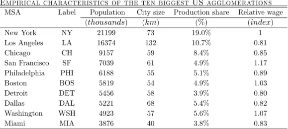
The study aims at providing information on the impact of spatial policies at the city scale on the climate change issue. The US is the geographical context for this study. We consider long-run general equilibrium paths for the US 20 largest cities. Table 2 summarizes the main spatial and economic features of the cities. We show model …ndings for two types of analysis concerning the interaction mechanisms between local (urban), regional (country) and global (world) economies and investigate those mechanisms in as many alternative policy scenarios. The base year used for policy scenario analysis is the 2001, and the overall study covers the period 2001-2100, in one year steps.
The …rst analysis considers a Business-As-Usual (BAU) scenario of the world economy and look at the spatial and economic patterns of US urban development when cities are let be part of the global system. In turn, the global system is both economically and environmentally in‡uenced by those patterns. In the BAU scenario, the major drivers of the (both US and world)
macroeconomy (e.g., population, labor productivity, oil price, primary energy mix, CO2 emissions) follow some conservative trend that are set in
Imaclim-R.
Next, local spatial policies are considered that a¤ect the urban spatial structure through augmented public expenditure in the local infrastructure sector. The direct e¤ect of infrastructure policy takes the form of increased urban density due to increased investments in the building sector and is an-alyzed in a speci…c infrastructure scenario. The e¤ect of such a spatial den-si…cation policy on global carbon emissions is also isolated, so as to assess its complementary city-scale e¤ect in reducing the cost of a broader inter-national climate policy that aims at setting a market price for carbon. The cost o¤-setting e¤ect of the two types of policy is addressed by comparing two low carbon scenarios in which an identical cap on carbon emissions is en-visaged. The ambitious climate policy requires a mix of carbon pricing (and other economic incentives) and speci…c “policies and measures”, among which densi…cation policies at the urban scale can either be planned or not.
A Long-run patterns of urban development
In the BAU scenario, the conservative assumption of a constant average den-sity (as de…ned by: Lj
2dj) in each agglomeration holds throughout the time
path considered. For the sake of presentation, we narrow the study of long-run (spatial and economic) patterns of urban development and present results for the ten largest US urban agglomerations.
The dynamic mechanisms of urban development are driven by the at-tractiveness index Aj a¤ecting …rm migration decisions (see …gure 1). The
number of active …rms nj in turn in‡uences the supply side of the market, as
measured by a variation in the production size of each agglomeration, njqj as
the amount of locally available …rms varies. In particular, our model shows that given the general trend of continuous domestic growth of the production predicted by Imaclim-R, the share of this production borne by the available agglomerations is expected to be positively related to the number of …rms op-erating in each agglomeration (see …gure 2).Note: Data source: US Census Bureau, 2000.
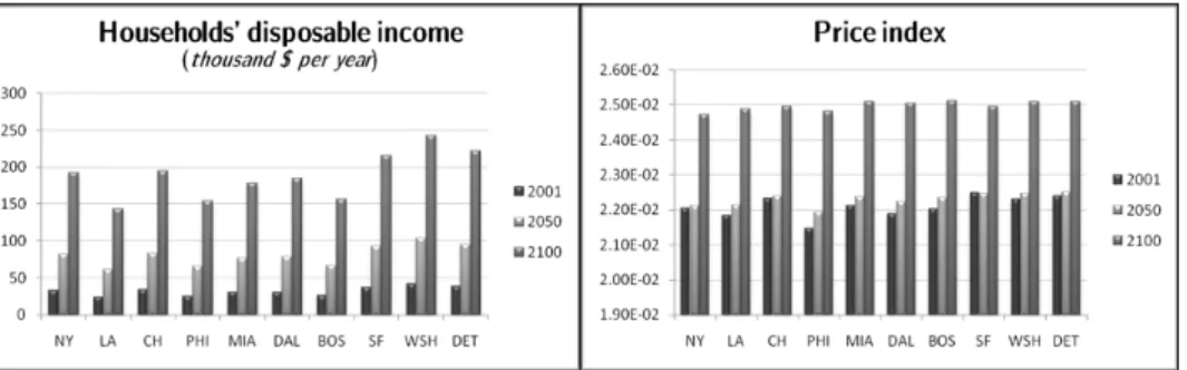
Changes in the size of production bring about modi…cations of the con-sumption behavior of individuals located in the agglomeration j. In partic-ular, changes in the consumption behavior occur via a modi…cation of the purchase power of households, as de…ned by j
Pj, which in turn results from a
combination of overall increasing households’disposable income j (conveyed
by labor productivity gains) and the cost of living in each agglomeration as captured by the price index Pj, which remains almost homogenous across the
agglomerations at each point in time (see …gure 3).
Finally, dynamic feedback mechanisms between the local and aggregate dimensions of the economy a¤ect the spatial structure of urban economies over the time. This e¤ect is captured through the study of the city size
Figure 1: Dynamic mechanisms of the urban market in terms of agglomeration attractiveness (left) and …rm migration (right). [Source: Imaclim-R modeling outcome based on US Census Bureau (2000) data]
Figure 2: Long-run domestic production size and pathways of production share allocation across cities. [Source: Imaclim-R modeling outcome based on US Census Bureau (2000) data]
Figure 3: Impact of urban development on onsumption behavior through households’ income (left) and price index (right). [Source: Imaclim-R mod-eling outcome based on US Census Bureau (2000) data]
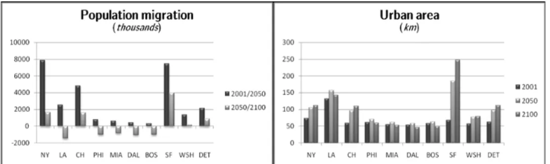
Figure 4: Spatial development patterns of cities through population dynamics (left) and urban land ares (right). [Source: Imaclim-R modeling outcome based on US Census Bureau (2000) data]
dj, which is a proxy for the extension of the urban land area. The size
of a given city evolves proportionally to the urban population Lj in this
BAU scenario. This is due to the assumption of constant average density in each agglomeration throughout the time period considered. Analyzing population migration ‡ows shows that on the one hand constant population growth path occurs for certain cities (New York, Chicago, San Francisco and Detroit); on the other hand, long-term population is found to decrease for the remaining ones (see …gure 4). This last result makes sense as the …rst group of cities experience a strong increase in the share of domestic production and therefore in their labor force requirement. Given our assumption on homogeneous density of the BAU agglomerations, New York, Chicago, San Francisco, and Detroit turn out to grow proportionally more than the others.
B Macroeconomic e¤ ect of urban policies
The US government decides to support densi…cation policies at the city scale that have the goal of reducing domestic dependence on energy import through lowering the need of transport. This type of policy takes the form of increased urban density in the 20 largest US cities. We test the e¤ect of the densi…ca-tion policy strategy on domestic and global macroeconomic setting through studying its impact on US national income and on global CO2 emissions,
re-spectively. From a modeling standpoint, this exercise is carried out by forcing an increasing trend on average urban density instead of assuming it constant as it is the case in the BAU scenario (see previous sub-section). Increased urban density in‡uences the general equilibrium through reduced travel de-mand. For the sake of simplicity, we consider a 25% increase of density for all agglomerations between 2010 and 2060, which corresponds to a moderate densi…cation rate of 0.45% per year. We abstract from any welfare e¤ect of increasing density. This is no shortcoming as we focus on carbon emissions that create external costs, which in turn harm social welfare.
the general equilibrium computation as the reduced external costs the policy induces. A …ve-year delay is assumed between the time at which investments are set in operation and their actual e¤ect on the urban structure.
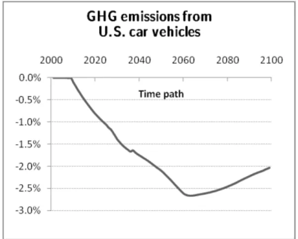
First we focus on the impact of increasing density on the use of automobile, which with its 90% of modal share represents the most important travel mode used for commuting purpose in US. Our …ndings reveal a bene…cial action of the policy measure in that it induces a reduction of carbon emissions by automobile displayed in …gure 5. Our model predicts that the overall e¤ect of a 25% densi…cation leads to 2% reduction of global CO2 emissions from car
use in 2100, passing through a 2.7% reduction in 2060.
Figure 5: Reduction of CO2 emissions from the automobile sector due to
in-frastructure policy at the urban scale. [Source: Imaclim-R scenario analysis]
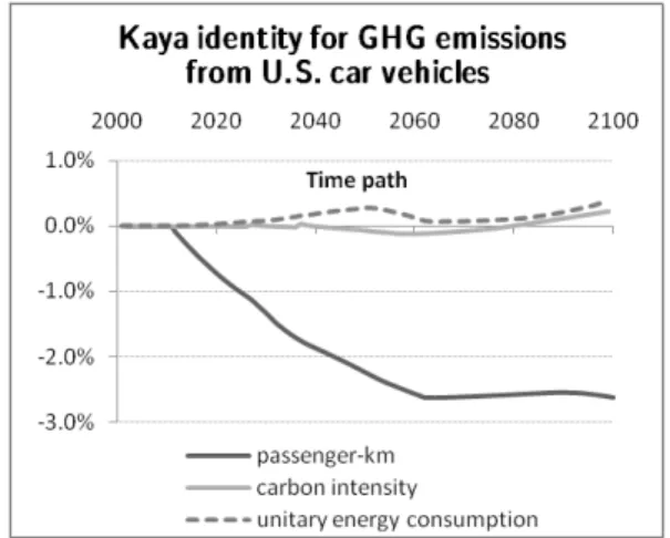
The drivers of a variation in carbon emissions from the transportation sector can be analyzed through what in the climate change literature is known as the “Kaya identity”:
Emissions = Emissions Energy
Energy
Transport volume Transport volume The above relation decomposes emission changes into components related to carbon intensity (in turn associated to the primary energy mix of liquid fuel production by oil, biomass, and coal), energy e¢ ciency of vehicles (resulting from technical change) and transport volume (measured in physical quantities, namely passenger-km).
Figure 6 shows relative variations of the three components of the Kaya identity when an densi…cation policy aimed at increasing urban density is set in place. Expectedly, the major impact of such a policy measure occurs through a reduction of the total volume of transport (measured in passenger-km) due to a decrease in average commuting distance by individuals in denser
agglomerations (around 2.6% reduction with respect to BAU case). However, indirect e¤ects also simultaneously occur that a¤ect carbon intensity and ve-hicle unitary fuel consumption in the long run. In particular, the decrease of liquid fuel demand due to a decrease in the average commuting distance, endogenously generates a fall of liquid fuel prices. This in turn slows down technical change towards more energy-e¢ cient vehicles (modeling …ndings show that automobile vehicles are 0.40% less e¢ cient in 2100), which ulti-mately causes the CO2 emissions from car to raise of another 0.6% in the
period 2030-2100 up to the …nal level of 2%.
Figure 6: Kaya decomposition of CO2 emissions from U.S. car vehicles.
[Source: Imaclim-R scenario analysis]
The positive net e¤ect of density on carbon emissions from cars is only partially o¤set by a simultaneous increase of emissions from other transport modes that is due to modal shift. In particular, our …ndings show that in-creasing density stimulates modal shift towards less energy-intensive travel modes. As a consequence, carbon emissions from public transport means are found to increase by 4% in 2100 (results for this analysis are not included here).
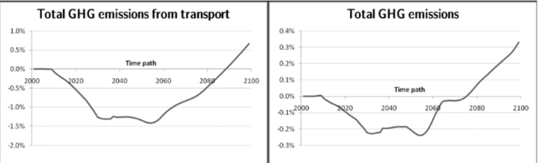
Results for the role of spatial policy measures on carbon emissions from the transportation sector and from all sectors of the US economy are reported in …gure 7, left and right panels, respectively. As a general insight, it is found that long-run emissions from transport may be higher if a densi…cation policy is implemented. This counter-intuitive outcome is a consequence of underlying general equilibrium mechanisms. Indeed, the reduced travel demand by au-tomobile pushes down the consumption of liquid fuels and, hence, their price due to release of market tensions. The associated fall of transport cost …nally stimulates a rise in transport activity, which in turn tends to o¤set the direct reduction of emissions from automobile induced by a 25% increase in urban density (see …gure 5). Figure 7 (right panel) shows that this indirect e¤ect may be dominant in the long run and induce an overall increase of emissions.
Figure 7: US trend for CO2 emission from the transportation sector (left) and
all sectors of the economy (right). [Source: Imaclim-R scenario analysis]
The trend for global total emissions (…gure 7, right panel) is of course similar but generally more diluted. This is due to the e¤ect of other energy-intensive economic sectors which are a¤ected but indirectly (i.e. through prices rather than quantities) by a spatial policy at the urban scale.
Next, the macroeconomic impact of setting in operation the densi…cation policy is studied. This is done through analyzing the long-run path of US total and sectoral GDP. The trend for US total domestic income under densi…cation policy scenario is studied with respect to the baseline one. Figure 8 reports results for this analysis.
Figure 8: Ratio of US GDP under infrastructure policy scenario to baseline US GDP. [Source: Imaclim-R scenario analysis]
As it is shown, in the …rst 30 years of the set in operation of the densi…ca-tion policy, early investments are responsible for losses in the overall economic activity, especially since a …ve-year delay is assumed before investments start to operate e¤ectively on urban density.
In 2060, the densi…cation process is ultimated, no additional investment is required, and the economy starts bene…ting from the full advantages of the densi…cation policy through a reduction of urban external costs. This
gives rise to a 65-year period during which the US GDP increases because of the bene…cial e¤ect of increased urban density in reducing national energy demand. In particular, up to the year 2060 and increasing-rate growth is envisaged for the US economy. In the last …ve years of our time period sim-ulation, this positive trend is expected to reverse. Main reason to that is the over-time decreasing trend of the price of energy due to fall in the energy de-mand, which is expected to slow down technical change and raise signi…cantly the energy intensity. This indirect e¤ect of the densi…cation policy becomes dominant in the last time period of the simulation, jeopardizing the initially bene…cial economic impact. Additional measures (like e.g., direct regulation for carbon emissions from vehicles) may be envisaged that can correct for the negative e¤ect of a rapid fall in energy e¢ ciency due to low energy demand.
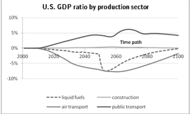
A sectoral analysis of the impact of densi…cation enables further insights for the comprehension of the underlying mechanisms through which the macro-economy is a¤ected. We consider the Imaclim-R 12 sectors of the world econ-omy. Figure 9 presents results for the impact of the spatial policy on four sectors of the US economy, the remaining 8 being a¤ected only marginally (within 0 and 0.5% of a variation in the GDP between the two scenarios has been found). These are all related to the US transportation sector.
Figure 9: Ratio of US GDP under infrastructure policy regime to baseline US GDP for four sensitive IMACLIM-R sectors. [Source: Imaclim-R scenario analysis]
As it is shown, production of liquid fuels is negatively a¤ected by a change in the spatial structure. This is logic consequence of the decrease in the use of car when density increases. Public transport and air transport show opposite trends. The increasing trend of the public transport is due to individuals’ preference towards cheaper and slower transport modes when car use drops and travel distances (and time) are shorter. The sharp increase of air trans-port in the second part of the period is stimulated by the overall lower price of liquid fuels under the densi…cation scenario than in the BAU one, which acts as a strong incentive for this energy-intensive mode.
additional public investments on buildings and transport. Hence, it stimu-lates the activity of sectors involved in densi…cation supply, among which construction plays a major role. This justi…es the higher sectoral GDP for the construction sector.
C Cost o¤ -setting e¤ ect of urban policies in the context of
international climate policy
As we have demonstrated in the previous sub-section, a densi…cation policy aimed at increasing urban density produces the net e¤ect of reducing carbon emissions. Therefore, we can expect to act as a valuable complementary mea-sure to carbon pricing schemes in the context of an ambitious climate policy. In this sub-section we test this. To investigate the role of urban densi…cation policies in a carbon constrained world, we assume that an international cli-mate policy is decided. For the sake of simplicity, we further assume that an agreement is reached among all countries to pursue the objective of a stabi-lization of CO2 atmospheric concentration at 450ppm, which corresponds to
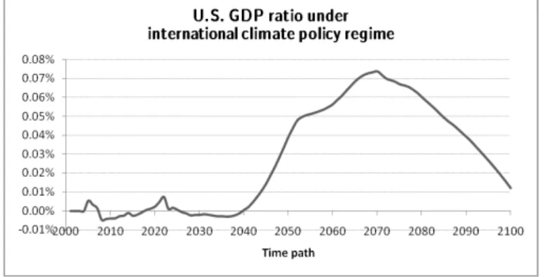
a carbon budget of 520GtC for the period 2001-2100. Burden-sharing across countries is based on a “contraction-and-convergence” principle, which aims at homogenous emissions per capita in 2100. Two alternative climate policy scenarios are considered with identical goal in terms of carbon emissions. Sce-narios di¤er regarding the implementation of a speci…c densi…cation policy at the urban scale as part of the “policies and measures”adopted to complement carbon pricing. We are interested in investigating whether a densi…cation pol-icy is bene…cial in this context. Results of the simulation show that this is globally the case (Figure 10).
Figure 10: Ratio of US GDP under infrastructure policy regime to US GDP under climate policy regime (e.g., carbon tax). [Source: Imaclim-R scenario analysis]
During the thirty-…ve …rst years, the densi…cation policy has hardly any e¤ect on the economic activity, early investments costs being compensated by the bene…ts of the densi…cation process. This policy at the urban scale is
speci…cally important in a climate policy context, since it induces a decrease of commuting emissions and then makes a lower carbon price compatible with the threshold on emissions. This e¤ect is dominant during the next 40 years and leads to a signi…cant increase of the economic activity when a densi…cation policy is carried out in urban areas as a complement of carbon pricing (around a 0.07% gain). In the last period, the densi…cation policy becomes less bene…cial in terms of economic activity as a result of its indirect e¤ect on energy intensity of the economy.
V
Conclusions
To summarize, this paper has presented a theoretical model in the light of the new economic geography (NEG) to explain the international policy com-munity’s claim of involvement of local governments (cities) in taking action against the global climate change. To provide better understanding of the feedback mechanism between urban, regional (country) and global (world) economies in the context of climate change, the model has been conceived to be driven in Imaclim-R, a dynamic, multi- region, computable general-equilibrium model for international climate policy analysis. It di¤ers from earlier work, which focused on a globally aggregated approach, by introducing production, consumption, trade and urban-related external costs for multiple cities within regions. Our study has allowed for regional economies where mul-tiple urban agglomerations dynamically evolve and alternative con…gurations of city growth potentially emerge. This has been done in a simple analyt-ical framework that enables to account for external (costs) bene…ts of land use and transport that re‡ect the (dis)economies arising from agglomeration. The spatial disaggregation of national into city economies is a major outcome of our research that goes beyond the scope of climate change analysis. Possi-ble applications concern the …eld of public economics and …nance, to analyze the macroeconomic consequences of interjususdictional mobility under some jurisdiction-speci…c land-use versus income tax. This line of research is not pursued here but may prove fruitful in future studies.
In addition to allowing for spatial disaggregation of the national economy, our model has departed from the standard NEG approach in at least two ways: i) dynamics of cities is allowed through migration decisions of …rms, whose location preferences go towards those urban agglomeration markets that o¤er the best investment opportunities. This in turn introduces a conceptual in-novation of our model that better …ts the modern structure of the production sector, where decisions are taken as a result of trade-o¤s between …rms’pro…ts and managers’and shareholders’interests; ii) the agglomeration spillover ef-fect is endogenously modeled by breaking the duality of the production sector through inclusion of a third input factor of production, namely the interme-diate consuption of goods. We consider intermeinterme-diate consumption as subject to external economies of scale resulting from improved production process through some agglomeration-speci…c technology spillovers. This allows for
analytically capturing the Marshallian-Chamberlanian set of positive spatial externalities, whose formalization in the broad literature of urban economics and trade theory has proved to be di¢ cult and controversial.
A speci…c study was carried out that accounts for the overall impact of the disaggregated US economy on the climate change. The study has consid-ered the U.S. …rst 20 largest cities in terms of population. We have compared three di¤erent strategies for the control of global warming through spatial pol-icy mechanisms: a market approach in which no climate change policies are taken; a domestic approach in which US country takes urban infrastructure (e.g., urban densi…cation) policies to raise its own national income through switching from high- to low-intensive carbon economy; and a global interna-tional approach in which all countries choose climate-change policy action and the US only fosters additional densi…cation policy that levies the burden of a carbon policy action. In the …rst baseline scenario, we assume that condition of constant average density in each urban agglomeration holds throughout the time path considered. In the last two scenario analyses, the densi…cation policy is thought as one that increases actual degree of density by 25% in 50 years (until 2060), which is moderate.
We have provided some guiding intuitions as well as evidence from cali-brated general equilibrium simulations that indicate that the spatial dimen-sion of the economy matters in the climate change debate. General equilib-rium results have shown that, …rst, in the business as usual (BAU) economy (market or uncontrolled scenario), the share of increasing-over-time produc-tion size is expected to be spread across the agglomeraproduc-tion proporproduc-tionally to the number of …rms operating in each agglomeration. This in turn pro-vokes modi…cations in the consumption behavior of individuals. In particular, purchase power of households increases as their disposable income increases, whereas the cost of living in each agglomeration proves not to vary signi…-cantly over the time period considered.
Second, we have studied the e¤ect of the densi…caiton policy strategy on domestic macroeconomic setting through studying the impact of increasing urban density on US national income. We have found that the major impact of such a policy occurs through up to 2.8% reduction of the total carbon emissions from transport due to a decrease in average commuting distance by individuals in denser agglomerations with respect to BAU case. Because of modal shift, the net bene…t of increasing density amounts to a total of 1.8% of carbon emission reduction. When looking at the total bene…t of a 25% increase in density in 2060, it is found that 0.35% reduction of cumulative CO2emissions from the overall US economy is reached. Next, we have studied
the impact of setting in operation the densi…cation policy on long-run path of U.S. GDP. In the …rst 30 years of the set in operation of the densi…cation policy, early investments are responsible for losses in the overall economic activity, especially since a …ve-year delay is assumed before investments start to operate e¤ectively on urban density. From 2030 to 2095 the economy is expected to bene…t from the advantages of the densi…cation policy via a
decrease of national demand to energy import. In the last …ve years of our time period simulation, this positive trend is reversed because of a fall in energy e¢ ciency due to low energy demand. As a consequence, households consume less of the di¤erentiated good and production falls, dragging down domestic income.
Third, we have investigated the cost-o¤setting role of the urban densi…ca-tion policy in the context of a carbon constrained world where countries are committed to stabilization goal of CO2atmospheric concentration at 450ppm,
which corresponds to a carbon budget of 520GtC for the period 2001-2100. Results have suggested a slow initial e¤ect of urban density on the economic activity. Subsequently, the spatial policy becomes e¤ective in decreasing com-muting carbon emissions and thus making a lower carbon price compatible with the threshold on CO2 emissions (around a 0.07% net gain in GDP). In
the last period of the policy, the densi…cation policy becomes less bene…cial in terms of economic activity as a result of its indirect e¤ect on energy intensity. More direct regulations of energy e¢ ciency may prevent long-run decreasing (yet positive) trend of national income. These …ndings have indicated that there will be substantial e¢ ciency in an densi…cation policy that intervenes to complement emissions control policies by reducing its total cost, when a market price for carbon is available.
In sum, the results of this integrated modeling analysis of climate and the spatial economy have emphasized the implications of the fact that while climate change is a global externality, the decision makers can be local and relatively small. The inherent di¢ culties involved in planning over a horizon of a century about so uncertain and complex a phenomenon like climate change may be avoided by integrating the international with the regional and urban dimensions of climate change policy, where externalities that lie at the origin of the phenomenon arise. This would allow in turn curtailing the risk of free-riding by non-participants or outdrawing in any global agreement due to the high cost of the carbon price policy.
References
[1] Armington, P.S. 1969. ‘A theory of demand for products distinguished by place of production’. International Monetary Fund Sta¤ Papers 16, 159-176.
[2] Böhringer, C., and A. Löschel. 2006. ‘Computable general equilibrium models for sustainability impact assessment: status quo and prospects’. Ecological Economics (in press).
[3] Ciccone, A. 2002.‘Agglomeration E¤ects in Europe.’European Economic Review 46, 213-227.
[4] Crassous, R., J-C Hourcade, and O. Sassi. 2006. ’Endogenous structural change and climate targets. Modeling experiments within Imaclim-R. The Energy Journal, 259-276. (Special Issue: ‘Endogenous Technological Change and the Economics of Atmospheric Stabilization’)
[5] Dixit, A.K., and J.E. Stiglitz. 1977. ‘Monopolistic competition and opti-mum product diversity’. American Economic Review 67, 297-308. [6] Fujita, M., and J-F. Thisse. 1996. ‘Economics of agglomeration’. Journal
of Japanese and International Economics 10, 339-378.
[7] Grazi, F., J.C.J.M. van den Bergh, and J.N. van Ommeren. 2008. ‘An Empirical Analysis of Urban Form, Transport, and Global Warming’. The Energy Journal 29(4), 97-107.
[8] Grazi, F., J.C.J.M. van den Bergh, and P. Rietveld. 2007. ‘Spatial Wel-fare Economics versus Ecological Footprint: Modeling Agglomeration, Externalities, and Trade’. Environmental and Resource Economics 38, 135–153.
[9] IPCC. 2001. ‘Climate Change 2001: The Scienti…c Basis’. D.L. Albritton et al. (eds.). Cambridge University Press, New York.
[10] Krugman, P. 1991. ‘Increasing returns and economic geography’. Journal of Political Economy 99, 483-499.
[11] Murata Y., and J-F. Thisse. 2005. ‘A simple model of economic geography à la Helpman–Tabuchi’. Journal of Urban Economics 58, 137–155. [12] OECD. 2006. ‘Competitive cities in the global economy’. OECD
Territo-rial Revies. Organisation for Economic Co-operation and Development, Paris.
[13] Paltsev, S., J.M. Reilly, H.D Jacoby, R.S. Eckhaus, J. McGarland, M. Saro…m, M. Asadoorian, and M. Babiker. 2005. ‘The MIT Emissions Prediction and Policy Analysis (EPPA) model: version 4’. MIT Joint Program on the Science and Policy of Global Change Report No. 125 (Aug.).
[14] Samuelson, P.A. 1952. ‘The transfer problem and transport costs: the terms of trade when the impediments are absent’. Economic Journal 62, 278-304.
[15] Solow, R. 1988. ‘Growth theory and after’. American Economic Review 78(3), 307-317.
[16] Tietenberg, T.H. 2003. ‘The tradable permits approach to protecting the commons: lessons for climate change’. Oxford Review of Economic Policy 19, 400-419.
[17] Thunen, von, H.J. 1966. ‘Von Thunen’s Isolated State’. (Translation by Wartenberg). C. M. Pergamon Press, Oxford.
Appendix
Here we provide the details of data calibration for the integrated modeling framework that has been developed in the paper. The twofold representa-tion adopted in Imaclim-R, both in money and physical ‡ows, creates some important constraints on calibration. Indeed, it makes necessary to use a so-called ‘hybrid matrix’ including consistent economic input–output tables and physical quantities (Sands et al., 2005). In the current version of the model, energy and transport sectors are described in explicit physical quan-tities (MToe and p-km, respectively). At the calibration date 2001, the equi-librium is obtained by combining macroeconomic data from GTAP 6, energy balances from ENERDATA 4.1 and the International Energy Agency (IEA) and data on passenger transport from (Schäfer and Victor, 2000). For each region, a set of macroeconomic variables corresponding to country-level aver-ages in 2001 are obtained as a result of this calibration process. Among those variables, we …nd domestic production size QC, production price pC, labor
requirements for production ClC, aggregate wage wC, price of intermediate
consumption goods pZ
C, intermediate consumption requirements for
produc-tion ZC and total production capacity KKC. The model presented in this
paper is calibrated to US data; since USA is a speci…c region of Imaclim-R, national averages at the USA level are directly given for all those macroeco-nomic variables.
The disaggregate microeconomies at the urban scale and the aggregate macroeconomy of the Imaclim-R equilibrium at the country scale are con-sistent if each variable appearing in both the scale description satis…es the condition: “the aggregation of microeconomic variables must equal the cor-responding aggregate macroeconomic variable given in Imaclim-R”. Given J agglomerations represented in USA, the condition on consistency sets that the set of equations listed in Table A1 must be veri…ed.