3.1.2 Design Catalogues: An Efficient Search Approach for Improved Flexibility in Engineering Systems Design

(1)

3.1.2 Design Catalogues: An Efficient Search Approach

for Improved Flexibility in Engineering Systems Design

The MIT Faculty has made this article openly available. Please share

how this access benefits you. Your story matters.

Citation Cardin, Michel-Alexandre, and Richard de Neufville. “3.1.2 Design Catalogues: An Efficient Search Approach for Improved Flexibility in Engineering Systems Design.” INCOSE International Symposium 23, no. 1 (June 2013): 62–83.

As Published http://dx.doi.org/10.1002/j.2334-5837.2013.tb03004.x

Publisher Wiley Blackwell

Version Author's final manuscript

Citable link http://hdl.handle.net/1721.1/93227

Terms of Use Creative Commons Attribution-Noncommercial-Share Alike Detailed Terms http://creativecommons.org/licenses/by-nc-sa/4.0/

(2)

Design Catalogues: An Efficient Search Approach for

Improved Flexibility in Engineering Systems Design

Michel-Alexandre Cardin

Department of Industrial and Systems Engineering, National University of Singapore Block E1A #06-25, 1 Engineering Drive, Singapore, 117576

macardin@nus.edu.sg

Richard de Neufville

Engineering Systems Division, Massachusetts Institute of Technology 77 Massachusetts Avenue, E40-245, Cambridge, MA, 02139, United States

ardent@mit.edu

Abstract. This paper proposes and demonstrates design catalogues as a computationally

efficient method for identifying improved designs for complex technological systems. This new process significantly speeds up the analysis of systems that will operate and will be managed under various uncertainty scenarios. It enables analysts to explore the design space more fully, taking into account a greater number of design parameters and variables. It can lead to design solutions with greatly improved lifecycle performance. The design catalogue consists of a small subset of designs that collectively perform reasonably well over a range of possible scenarios. The catalogue approach contrasts with the usual approach that optimizes designs for each scenario, and thus can only afford to examine a limited number of situations. Each design in the catalogue consists of combinations of design variables, parameters, and flexibility decision rules. The set of designs in the catalogue is determined using adaptive One-Factor-At-a-Time (aOFAT) analysis. An example demonstrates the use and how it leads to improved lifecycle performance compared to a standard benchmark design.

Introduction

Engineering systems are characterized by a high degree of technical complexity, social intricacy, and elaborate processes aimed at fulfilling important functions in society (ESD 2011). Given they are typically long-lived (+20 years), they face much uncertainty at strategic, tactical, and operational levels. Examples engineering systems include critical infrastructures for defense, emergency services, power generation and distribution, telecommunications, transportations, and housing.

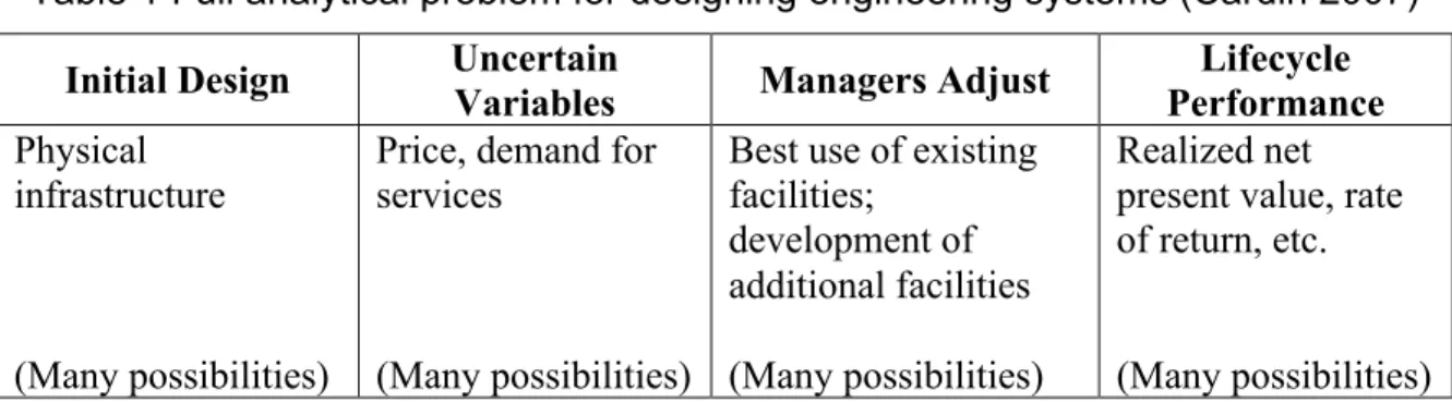
From a computational standpoint, the design of engineering systems today is a daunting task (Braha, Minai, and Bar-Yam 2006; de Weck, Roos, and Magee 2012). As summarized in Table 1, it involves modeling and optimizing basic infrastructures (e.g. plants, networks, etc.) considering a wide array of uncertainty scenarios (e.g. market demand, price, regulations) over long-term horizons. There can be many possible architectures and operating modes (e.g. number and size of plants, routing of vehicles on network, allocation of production lines to products, etc.) The system can also be evaluated based on many lifecycle performance indicators (e.g. net present value (NPV), return on investment (ROI), etc.) It is practically intractable to consider exhaustively all possible design combinations and alternatives.

(3)

Table 1 Full analytical problem for designing engineering systems (Cardin 2007)

Initial Design Uncertain _Variables Managers Adjust _PerformanceLifecycle

Physical infrastructure

(Many possibilities)

Price, demand for services

Best use of existing facilities;

development of additional facilities (Many possibilities)

Realized net present value, rate of return, etc. (Many possibilities) A typical approach in engineering design and complex project evaluation is to simplify the full analytical problem. Instead of considering many scenarios of periodical data, designs are often optimized for the most likely projection of major uncertainty drivers (Braha, Minai, and Bar-Yam 2006; Eckert et al. 2009). Typical project evaluation approaches based on discounted cash flow (DCF) analysis, such as NPV, does not account for the fact that system operators will react periodically to enhance the system performance (Trigeorgis 1996). Also, design decisions are often based on one evaluation metric like internal rate of return (IRR), NPV, or ROI. The combination of such practices in systems design and evaluation can lead to sub-optimal choices, and even economic failure (Cardin et al. 2012).

Flexibility in Engineering Systems Design:

Computational Challenges

There has been a great deal of effort over the last two decades to improve standard design and evaluation practice by making more explicit considerations of uncertainty. Flexibility in engineering design is one approach, which aims at designing an engineering system so it can adapt and change pro-actively in the face of uncertainty in environment, markets, regulations, and technology (de Neufville and Scholtes 2011; Nembhard and Aktan 2010). It is a different design paradigm from, for example, design for robustness, which aims at making systems function more consistent and invariant to changes in the environment, manufacturing, deterioration, and customer use patterns (Jugulum and Frey 2007). In the literature, flexibility in design is often referred to as a real option embedded “in” the system (Mikaelian et al. 2011; Wang and de Neufville 2005). Flexibility can improve expected lifecycle performance by affecting the distribution of possible outcomes. It reduces the effect from downside (like buying insurance), risky scenarios, while positioning the system to capitalize on upside, favorable opportunities (like buying a call stock option). For example, the 25 de Abril bridge connecting Lisbon to the municipality of Almada in Portugal was originally designed to carry four car lanes. Engineers accommodated the design for more car lanes if needed in the future, as well as a railway on its lower platform, should usage and demographic patterns warrant it. This flexibility in design later allowed expansion to the current six car lanes and two-railroad tracks infrastructure seen today. This strategy required a smaller initial investment than if full capacity was deployed, and deferred additional costs to the future, taking advantage of the time-value of money. It also enabled more traffic between the two cities today, contributing to a growing economy.

Flexibility has shown improvements typically ranging between 10% and 30% compared to the outcome from standard design and evaluation practice in different industries: strategic phasing of airport terminals development (de Neufville and Odoni 2003; Gil 2007), offshore platforms designed for future capacity expansion (Jablonowski, Wiboonskij-Arphakul, and Neuhold 2008), strategic investments in new nuclear plant facilities (Rothwell 2006), supply

(4)

chain adaptation to fluctuating exchange rates (Nembhard, Shi, and Aktan 2005), strategic investment in innovative water technologies (Zhang and Babovic 2012), etc. Examples abound.1

An important issue in designing engineering systems for flexibility is the complexity of the analytical problem. In addition to the many design variables and parameters to consider, designers need to account for a wide range of uncertainty scenarios, periodic managerial adjustments, and evaluation metrics. The case of Lin et al. (2009) illustrates the issue, working on the design of an oilrig with a major oil company. The company would use a highly complex model for the oil and gas infrastructure system, and optimize the design based on average historical price, and most likely original oil in place (OOIP) quantity (i.e. estimated reserves). Optimization for only one combination of oil price and OOIP scenario would require at least a day of intensive computations. If only three distinct price scenarios were considered in each year of a 20-year lifecycle (i.e. typical lifetime for such asset), the number of design configurations to investigate would be 320_{~3.5 billion. Consideration of so}

many scenarios is, as a practical matter, intractable, let alone with additional degrees of freedom stemming from explicit considerations of flexibility in design and management. In essence, the problem addressed in this paper is that the analysis of performance of an engineering system under uncertainty requires a special design or operating plan for each scenario. The definition of such plans and their lifecycle performance requires a lot of time and analytical resources, as exemplified above, so analysts can only look at a very few designs fully. Therefore, solutions possibly improving lifecycle performance cannot be examined due to time and analytical constraints.

Proposed Solution

This paper addresses this issue by devising a priori a set of operating plans or models that together deal reasonably adequately with a range of uncertainty scenarios. This speeds up the analysis for the most relevant plans, allows analysts to consider more design alternatives, and enables uncovering better design solutions with improved lifecycle performance. The proposed solution suggests a middle-ground approach standing between the simplest set of assumptions typically made in design and evaluation, and the full analytical problem summarized in Table 1. It relies on a representative range of possibilities small enough to be manageable analytically, and broad enough to enable a more informed analysis of the design problem. The aim is to provide a practical approach leading designers to rapid lifecycle performance improvements by explicit considerations of flexibility. It is also efficient in terms of the computational and analytical resources required.

Design Catalogues. The method simplifies the analysis by relying on the concept of a design

catalogue. The catalogue provides a limited number of scenarios and responses intended to describe relevant patterns designers might wish to anticipate. An operating plan is therefore a combination of design variables, parameters, and flexible decision rules to manage the engineering system in operations, and over its lifecycle. For instance, instead of considering explicitly all possible 3.5 billion price scenarios, only a handful representative scenarios are considered. One operating plan is created to suit each scenario, thereby creating the catalogue.

1_{More case studies are available at http://ardent.mit.edu/real_options/Common_course_materials/papers.html,}

(5)

Representative uncertainty scenarios can be selected based on different criteria, and operating plan crafted to deal best with each scenario. For example, consider a scenario where prices rise steadily at first, and start falling after some time. Another possibility is for prices to start low for the first few years, and then incur a sudden surge due to high demand. Volatility around the main trend may vary between low, medium, and high values. In each case, a different flexible response might be required, and better supported by a different flexible design configuration. The catalogue contains the flexible design alternatives that cope most appropriately with each scenario.

The concept of catalogue is analogous to customers buying suits, typically coming in many sizes and shapes. While it is possible to hand-tailor suits for each customer, this can be demanding in terms of manufacturing and operations. One alternative is to have a range of suits (i.e. a catalogue) that will reasonably fit any of the customers’ needs. The items in the catalogue provides a range of choices varying along several dimensions – as in the example below Table 6 – and as in real life (e.g. tall, short, large, thin, etc.).

Decision Rules. A decision rule defines the trigger point or mechanism at which time it is

appropriate to exercise a designed flexibility. It aims to simulate an appropriate decision taken by the system operator or manager at any given point in time to adapt the system to arising conditions. Such rule is typically based on the observation of a given uncertainty source (e.g. demand, price, technological performance) to which the system is called to react. It is crucial for determining the lifecycle performance improvement and value-added by flexibility compared to standard design approaches. In the example of the 25 de Abril bridge, a hypothetical decision rule could have been that if traffic demand reached a certain threshold, additional lanes would be added. If traffic demand increased even further, this would warrant development of the railroads on the lower platform. While it is unclear what decision rule was used in this case, it is clear that the decision to expand capacity was based on observed changes in the main uncertainty drivers (e.g. availability of EU funds, prospects of land boom on South shore, etc.) Decision rules aim at capturing such managerial decisions to be included in the modeling.

A decision rule simplifies the analysis compared to full optimization on each uncertainty scenario. This is because it only requires “looking back” over the information provided up to a certain point in time. Typical stochastic or dynamic programming algorithms used in standard real options analysis (Copeland and Antikarov 2003; Dixit and Pindyck 1994) consider the best sequence of decisions over the entire scenario period. On the one hand, this may not be realistic in an engineering context because a decision-maker does not know a priori how the future will unfold. Also, the number of possible combinations explodes exponentially as a function of the number of time periods – or stages – also making the problem quickly intractable.

Design Space Exploration. The aim of the proposed approach is to reduce the complexity of

the analysis. It focuses on investigating a suitable combination of physical design variables and parameters together with flexible decision rules available to better handle uncertainty. This abstract combinatorial space is referred in this paper as “design space”. The approach structures the process of exploring the design space under considerations of uncertainty and flexibility, while still being tractable computationally.

The exploration process is inspired from the adaptive One-Factor-At-a-Time (aOFAT) fractional factorial algorithm by Frey and Wang (2006) used in statistical design of

(6)

experiments (DOE). The approach consists of starting at a particular design combination (or factor level), and measuring the lifecycle performance obtained using a system model. One of the factor levels is then toggled to another level, and another performance measurement is taken. If the objective function is improved, the change is kept, and the analysis moves on to toggling another factor and level. If the response is not improved, the change is discarded, and another factor level is explored. The algorithm goes in sequence until all factors levels have been explored once.

This process reduces the number of search iterations tremendously, while still reaching a good solution. Frey and Wang (2006) showed that in a design space with n factors with 2-levels each, aOFAT reduces the number of experiments from 2n to n + 1, while still reaching on average nearly 80% of the optimal response. The main motivation for using aOFAT is the good tradeoff it provides between computational efficiency and precision. The remainder of the paper is organized as follows. In the next section, a short review of the literature is presented to highlight previous efforts in addressing this computational design problem. The methodology section explains how the design catalogue is developed, and how to evaluate flexible design alternatives. An example application is presented for the analysis of a public infrastructure system. Results, findings, validity, and limitations of the framework are discussed, together with possible avenues for future research, followed by conclusions.

Literature Review

Conceptual Process

The conceptual process of designing engineering systems for flexibility typically requires five phases depicted. The process starts from an initial design, obtained by means of existing and/or standard design procedures (phase 1). This phase is necessary to circumscribe the initial design space, as it is difficult to consider flexibility without an initial design. A review of current procedures to generate initial design alternatives is provided by Tomiyama et al. (2009). The major uncertainty sources affecting lifecycle performance are recognized, modeled, and incorporated explicitly in the process (phase 2). Flexibility strategies are generated to deal with these uncertainties, and enablers are identified in the design (phase 3). The design space is explored systematically to find flexible design alternatives leading to improved lifecycle performance, as compared to the baseline design (phase 4). Phase 5 oversees phases 1-4 to create a productive collaborative environment for designers. More details on this process and suitable procedures for each phase are provided in Cardin (2012).

Design Space Exploration

This paper is mainly concerned with design space exploration (phase 4). This phase involves developing efficient computational methods and search algorithms to find the most valuable flexible design configurations, subject to a range of design variables, parameters, decision rules, and uncertainty scenarios. This phase requires modeling explicitly the flexible design concepts generated in phase 3. For example, the flexible design concept explored in the case of the 25 de Abril bridge is capacity expansion. This could give rise to a wide range of flexible design alternatives with different decision rules. One could design additional capacity for one, two, or three extra lanes when user demand reaches threshold T, account for one or two additional rail tracks, etc. Given T alone can take on any value, there is are infinite combinations of physical design variables and decision rules, each leading to a different lifecycle performance outcome. The design procedures in phase 4 provide systematic ways to search effectively through this combinatorial space.

(7)

The methods in phase 4 typically integrate real options analysis tools based on dynamic programming and economics (Bellman 1952; Cox, Ross, and Rubinstein 1979; Dixit and Pindyck 1994; Trigeorgis 1996) with standard optimizations and statistical techniques to assess the lifecycle performance of flexible design alternatives. To tackle this computational problem, Jacoby and Loucks (1972) first suggested screening methods to identify most promising design alternatives within reasonable time. de Neufville and Scholtes (2011) suggested three types of screening methods: bottom-up, simulators, and top-down. Bottom-up models use simplified versions of a complex, detailed design model. Simulators incorporate statistical techniques (e.g. response surface modeling) and/or fundamental principles to mimic the response of the detailed model. Top-down models use representations of major relationships between the parts of the system to understand possible system responses (e.g. systems dynamics).

Wang (2005) was first to apply screening methods for design space exploration in the context of flexibility. He applied his approach to the analysis of water infrastructures in China. Lin (2009) developed a bottom-up screening model of an integrated oil and gas system to identify valuable flexible design alternatives in an offshore oil platform system. Yang (2009) used a response-surface methodology coupled with fractional factorial analysis to explore flexibility in the car manufacturing process. Hassan and de Neufville (2005) used genetic algorithms to structure the search process in oil platform design and planning. Olewnik and Lewis (2006) extended a utility-based framework to the context of flexibility in product development. Ross (2006) proposed Multi-Attribute Trade space Exploration (MATE) based on Pareto-optimal configurations. This process exploits tradeoffs between design performance utility attributes, and lifecycle cost.

Research Gap

The methods above all depend on simplifications of a system model. Simplifications, however, can be a difficult to achieve for many reasons, depending on the context. For example in bottom-up methods, it may be unclear what parameters to simplify. Should designers simplify considerations of demand and price to make the model run within reasonable time? Are there other factors more important to consider? In the case of simulators, it is unclear what is the best sampling mechanism to create the response surface. Different sample points may lead to different response surfaces, and different optimal design solutions. In top-down models used in systems dynamics, a deep understanding of the system’s underlying feedback and feedforward mechanisms is required (Sterman 2000). Building such model requires intensive field research and data collection (Steel 2008), which can be constraining. In addition, for a variety of practical reasons (e.g. time and resource constraints), there might be situations where practitioners cannot use screening methods. In this case, it might be better to work directly from the model at hand, even if the model has high complexity. The methodology detailed in the next section introduces a complementary and practical way to address the above issues.

Methodology

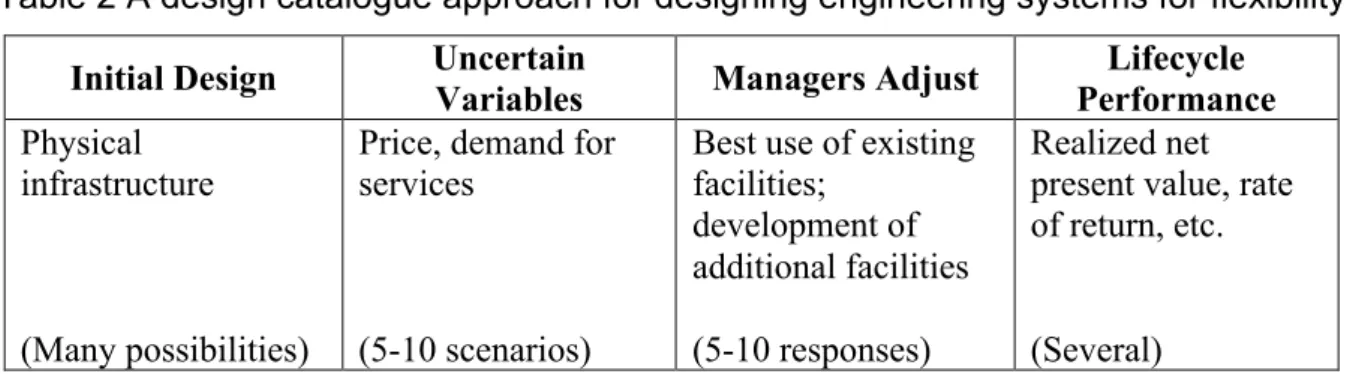
Table 2 below summarizes the design catalogue approach. The approach considers a handful of representative uncertainty scenarios (e.g. 5-10) and associated flexible responses to each scenario. The catalogue approach enables designers to consider several lifecycle performance metrics, depending on the decision-making environment.

(8)

Table 2 A design catalogue approach for designing engineering systems for flexibility

Initial Design Uncertain _Variables Managers Adjust _PerformanceLifecycle

Physical infrastructure

Price, demand for services

(5-10 scenarios)

Best use of existing facilities;

development of additional facilities (5-10 responses)

Realized net present value, rate of return, etc. (Several) The general methodology for developing a design catalogue has five steps:

1- Develop a basic model for measuring lifecycle performance

2- Find representative uncertainty scenarios affecting lifecycle performance 3- Identify and generate potential sources of flexibility in design and management

4- For each uncertainty scenario, find the most appropriate flexible operating plan and construct the catalogue using the aOFAT fractional factorial algorithm

5- Assess lifecycle performance improvement – if any – using the design catalogue as compared to the baseline design under uncertainty

Analysis and Results

This section demonstrates application of the five-step process. The objectives are to demonstrate that the design catalogue technique 1) can improve expected lifecycle performance compared to a baseline design typically more rigid (i.e. inflexible), and 2) is computationally efficient compared to an exhaustive search. The former objective demonstrates the value of embedding flexibility in engineering systems. The latter shows that the technique is useful particularly when computational efficiency is required.

Case Study

The case study is inspired from the development of a multi-level parking garage near the Bluewater commercial center located in the surrounding of London, United Kingdom. The analysis is based on the model presented in de Neufville et al. (2006). Following a process similar to that described in the Conceptual Process section, the authors showed that flexibility embedded in the design improved expected lifecycle performance compared to a more rigid, baseline design. The baseline design would account for six initial floors, providing the optimal NPV based on the most likely forecast of parking space demand.2 Embedding flexibility in the design enabled capacity expansion when demand was higher than installed capacity. This flexibility was enabled physically by building stronger columns to support additional floors.

The authors showed that the main source of value was the ability to expand capacity when needed. A smaller initial design with four floors instead of six would prevent unnecessary investments in unused capacity. This would lower initial capital expenditures and exposure to downside risks in case demand was weaker than expected. It would also position the system to capture upside opportunities, in case more demand materialized. The authors showed a clear improvement in expected lifecycle performance (i.e. E[NPV]) for this design strategy,

(9)

as compared to an inflexible six-floor design. The evaluation approach led to a completely different design (i.e. four initial floors with stronger structure and columns to support expansion) than one based on a standard design approach. The authors only explored the value of one decision rule, however, which was to expand when demand exceeded capacity for two consecutive years. They did not explore other combinations of decision rules and design variables. Application of the design catalogue technique shown next enables a more thorough exploration of this design space.

Application

Step 1: Basic Model Development. Application of the catalogue approach starts from the

development of a basic model enabling quantitative lifecycle performance assessment of design alternatives. Here, an economic DCF model is used, inspired from the data reported in de Neufville et al. (2006), and summarized in Appendix (Table 8). Net present value (NPV) is the objective function (O) for measuring economic lifecycle performance of different design alternatives. The model implements the following relationships between the design variables (DV), design parameters (DP), and constraints (C):

NPV = Rt− Ct (1+ r)t t=0 T

∑

( 1 ) Rt = min(Dt, kt)p, t ≥ 0 ( 2 ) kt= n0 ft t=0 T

∑

( 3 ) kt ≤ n0fmax, t ≥ 0 ( 4 ) C0 = cc0 + cf + cl ( 5 ) Ct = ktcr + cl + ce, t > 0 ( 6 ) Dt = Df – αe-βt ( 7 )

Equation 1 shows how to compute NPV, which is the sum of DCF. Equation 2 states that revenues in any given year t are capped by installed capacity kt. Equation 3 constrains

installed capacity kt at time t to be the sum of parking spaces built in each previous years,

plus the number of floors ft added at time t. In the inflexible system, k0 = n0f0, the initial

capacity of the system, and ft = 0 ∀ t, since no expansion is possible. For the flexible system

described in step 3 below, ft ≠ 0 because expansion may occur as demand changes. Equation

4 explains that the total number of floors is capped at fmax such that kt in any given year does

not go beyond n0fmax. Equation 5 shows that cost at year 0 (C0) is given by the total

construction cost cc0, the cost of acquiring the flexibility to expand3 cf (i.e. the stronger

columns), and the cost of leasing land cl. The total construction cost cc0 = n0f0cc for the first

two floors, and then grows at rate gc = 10% for all floors above two. Equation 6 shows that

3_{Note that c}

f = 0 in this model for simplification purposes. The reason is that the model assesses the value of flexibility

assuming that the flexibility is available. The real value of a design thus takes the measured NPV and subtracts from it the real acquisition cost of the flexibility. As long as this difference is positive (i.e. NPV – cf (real) > 0), it is worth incorporating

(10)

total cost Ct includes recurring operating cost ktcr, land leasing cost cl, and expansion cost ce.

Variable cc is measured based on the growth in construction cost gC times the number of

additional parking space built at time t. Deterministic demand for parking space Dt in year t is

modeled using Equation 7, where α = additional demand by project midlife (year 10) + additional demand by final year (year 20), β = - ln(additional demand by year 10/α) / (10 – 1), and Df is final demand at year 20. The model assumes that D1 = 750 parking spaces,

additional demand by year 10 = 750, and additional demand by final year = 250, such that α = 1,000 and β = 0.15. Under this framework, an example design vector for the inflexible system is simply f0, the initial number of floors. Here ft = 0 for ∀ t, and therefore kt = k0. The

optimal design has six floors (f0* = 6), leading to NPV = $10.6 million.

Step 2: Finding Representative Uncertainty Scenarios. This step finds a representative set

of scenarios for the major uncertainty sources affecting lifecycle performance. It also incorporates stochasticity in the basic model, using the following equation:

Dt+1S = gt(1 + Dt) ( 8 )

In Equation 8, Dt is calculated as before, although now D1, additional demand by year 10, and

additional demand by final year are random variables sampled from a uniform distribution with values ± 50% off the initial projection. Inter-annual demand growth gt is modeled using

Geometric Brownian Motion (GBM): gt = gpdt + σdWt√dt, where gp = Dt/Dt-1 – 1 is the

projected inter-annual demand growth obtained using the stochastic version of the demand model, dt = 1 year time increment, σ = 15% is the assumed volatility of demand. Variable dWt is the standard Wiener process, in this case sampled from a uniform distribution U ~ (-1,

1) instead of a normal distribution for better computational efficiency. Using this model, the rigid design (f0* = 6) gives rise to an average NPV (or expected NPV, ENPV) ENPVinflex. =

$7.0 million under 2,000 stochastic demand scenarios.

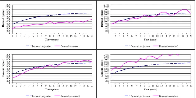
Figure 1 shows a handful of example scenarios alongside the most likely deterministic demand scenario modeled in step 1. At the moment there is no systematic approach to select a representative set of uncertainty scenarios, besides relying on expert inputs. Readers are referred to Morgan and Henrion (1990) for more systematic techniques to elicit scenarios and probability distributions. For demonstration purposes, these authors suggest looking at the growth occurring in initial years 1-5. These years are crucial as demand is assumed to taper off to an asymptotical value in year 20.

The approach here is to split scenarios into five growth categories. Five growth parameters β are shown in Table 3, giving rise to the representative scenarios in Appendix Figure 6. The percentage increase is calculated from the realized demand scenario. The mid-values provide a breaking point to assign one stochastic scenario to one category. For example, stochastic scenarios with growth above mid-value 123% in years 1 to 5 will be assigned to category 1, while scenarios with growth less than 38% will be assigned to category 5.

(11)

0! 200! 400! 600! 800! 1000! 1200! 1400! 1600! 1800! 2000! 2200! 2400! 1! 2! 3! 4! 5! 6! 7! 8! 9! 10! 11! 12! 13! 14! 15! 16! 17! 18! 19! 20! D eman d (s p ac es )! Time (years)!

Demand projection! Demand scenario 1!

Figure 1 Example demand scenarios generated using the stochastic demand model alongside the most likely demand projection

Table 3: Categories of representative demand scenarios based on percentage increase from years 1 to 5

Category Growth parameter β Percentage increase Mid-value 1 0.990 131% 123% 2 0.500 115% 100% 3 0.250 84% 68% 4 0.125 52% 38% 5 0.050 24%

Step 3: Identify/Generate Flexibility in System Design and Management. This example

focuses on the flexibility to expand capacity, extending the work by de Neufville et al. (2006). While there are many design procedures available to look systematically into flexible strategies and design enablers, these are taken from the previous study to satisfy the needs of the demonstration, and for brevity. Generating flexibility and identifying enablers in design are in fact topics of active research (Cardin 2012).

The design vector for the flexible system is: [a1-4, a9-12, a17-20, dr, ft, f0]. This vector includes

both decision rules and design variables. Decision rules are described conceptually for brevity. They are implemented using logical programming statements in Excel® – i.e.

IF(logical condition, outcome if true, outcome if false). Decision rules a1-4, a9-12,

and a17-20 state respectively whether it is possible or not to expand capacity during years 1-4,

9-12, and/or 17-20 by taking binary values (Yes = 1, No = 0). It may not make sense for some decision-makers to allow expansion in the early years of the project, or at the end. Similarly, some decision-makers may prefer not to allow expansion in years 9-12 to study mid-life evolution of the project. Decision rule dr states how many consecutive years demand must be higher than installed capacity to allow expansion. For example, dr = 1 means a (risk-seeking) decision-maker will observe demand for just one year and will go ahead with expansion if demand was higher than installed capacity. The design variable ft states how

(12)

many floors are added at each expansion phase. These decision rules are applied at the end of every year, and provide alternatives to suit risk-averse, risk-neutral, and risk-seeking decision-makers. They do not, however, represent all possible decision rules available for this design problem, but possible examples to demonstrate the catalogue technique.

Many combinations of decision rules and design variables exist to enable and manage the flexibility, each leading to a different operating plan. It is not clear what combination or operating plan gives better lifecycle improvement compared to a fixed design. Furthermore, one operating plan may be well suited for a particular demand scenario, but not necessarily for another. It is better to adapt the operating plans depending on uncertainty outcomes. Table 4 summarizes the flexible decision rules and design variables – also called factor – used in this example application, leading to 33 x 23 = 216 possible operating plans. A level refers to the value a decision rule and/or design variable can take.

Table 4: Summary of flexible decision rules and design variables (i.e. factors) investigated in this study. Each combination leads to one operating plan

DVs and

DRs Factor Description

Levels

- o +

a1-4 Expansion allowed in years 1-4 No Yes

dr Expansion decision rule (years) 2 3 4

ft Number of floors expanded by 1 2 3

f0 Number of initial floors 4 5 6

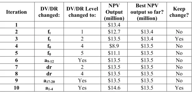
Step 4: Construct the Design Catalogue. aOFAT is used to accelerate the search process for

the design catalogue. The exploration process for example scenario 1 in Figure 6 (see Appendix) is summarized in Table 5. The initial design and exploration sequence are selected randomly, as suggested by Frey and Wang (2006). The baseline operating plan is described by the vector [a1-4, a9-12, a17-20, dr, ft, f0] = [No, No, No, 3, 3, 6].

Table 5: Description and output of each iteration in the aOFAT sequence

Iteration _changed:DV/DR DV/DR Level _{changed to:}

NPV Output (million) Best NPV output so far? (million) Keep change? 1 $13.4 2 ft 1 $12.7 $13.4 No 3 ft 2 $13.5 $13.4 Yes 4 f0 4 $8.9 $13.5 No 5 f0 5 $11.1 $13.5 No 6 a9-12 Yes $13.5 $13.5 No 7 dr 2 $13.5 $13.5 No 8 dr 4 $13.5 $13.5 No 9 a17-20 Yes $13.5 $13.5 No 10 a1-4 Yes $14.6 $13.5 Yes

(13)

The initial vector produces NPV = $13.4 million using the baseline model in step 1. Decision rule factor ft is changed from value ft = 3 to ft = 1, leading to NPV = $12.7 million. Since the

response is not improved, the decision rule is set back to its original value, and then the response using ft = 2 is measured. Since NPV = $13.5 million is an improvement compared to

the initial design vector at NPV = $13.4 million, ft = 2 is kept. The analysis then moves on to

other design variables and decision rules, until all factor levels have been explored once. The operating plan for scenario 1 is described by vector [a1-4, a9-12, a17-20, dr, ft, f0] = [Yes, No,

No, 3, 2, 6]. This operating plan states that if demand grows very fast in early years, capacity expansion should be allowed in years 1-4 only if demand is higher than installed capacity for three consecutive years, be done two floors at a time in each expansion phase, and start with an initial design of six floors to capture as much capacity as possible. Preparing for fast expansion makes sense intuitively for scenario 1, since it has the fastest initial growth. The same approach is used to generate a flexible operating plan for each representative demand scenario. This leads to the complete design catalogue summarized in Table 6.

Table 6: Design catalogue

DVs and DRs Op. Plan 1 Op. Plan 2 Op. Plan 3 Op. Plan 4 Op. Plan 5

a1-4 Yes Yes Yes Yes No

a9-12 No Yes Yes Yes Yes

a17-20 No No No No Yes

dr 3 2 2 2 4

ft 2 2 2 1 1

f0 6 6 4 4 4

Step 5: Evaluate the Lifecycle Performance of the Catalogue. This step simulates the

ability of the system operator to choose between different flexible operating plans, based on demand observations. Figure 2 shows an example stochastic scenario alongside the original demand projection. Since growth is about 35% between years 1-5 (from 690 to 931), this scenario is associated to operating plan 5.

0! 200! 400! 600! 800! 1000! 1200! 1400! 1600! 1800! 2000! 2200! 2400! 1! 3! 5! 7! 9! 11! 13! 15! 17! 19! D eman d (s p ac es )! Time (years)!

Demand projection! Demand scenario!

Figure 2 Example simulated demand scenario assigned to operating plan 5 Figure 3 shows the lifecycle effect of the operating plan on an Excel® implementation of the DCF model, leading to NPV = $17.4 million. Even though the operating plan is relatively

(14)

conservative in the first few years by making expansion difficult, it still enables an aggressive series of expansion (fourth row from top) after year 5, as demand picks up later.

A Monte Carlo simulation is performed with 2,000 demand scenarios. Each scenario is associated to one of the five operating plans. The design variables and decision rules associated to an operating plan lead to a different sequence of expansion for each scenario, leading each time to a different NPV outcome.

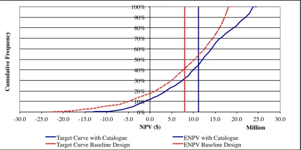
Figure 4 shows the cumulative distribution functions – also referred as target curves – for the most valuable inflexible baseline design with six floors, and using the design catalogue. The target curve resulting from the catalogue approach dominates stochastically the one from the inflexible 6-floor design.

Year 0 1 2 3 4 5 6 7 8 9 10 Realised demand 690 733 964 1,088 931 986 1,104 1,310 1,420 1,305 Capacity - 800 800 800 800 800 800 1,000 1,200 1,400 1,600 Expansion? expand expand expand expand

Expansion (using expansion operating plan)?

Build extra capacity 0 0 0 0 0 0 200 200 200 200 0 Revenue $0 $6,900,000 $7,333,222 $8,000,000 $8,000,000 $8,000,000 $8,000,000 $10,000,000 $12,000,000 $14,000,000 $13,050,245 Operating costs $0 $1,600,000 $1,600,000 $1,600,000 $1,600,000 $1,600,000 $1,600,000 $2,000,000 $2,400,000 $2,800,000 $3,200,000 Land leasing costs $3,600,000 $3,600,000 $3,600,000 $3,600,000 $3,600,000 $3,600,000 $3,600,000 $3,600,000 $3,600,000 $3,600,000 $3,600,000 Expansion cost $0 $0 $0 $0 $4,259,200 $4,685,120 $5,153,632 $5,668,995 $0 Cashflow $0 $1,700,000 $2,133,222 $2,800,000 $2,800,000 $2,800,000 -$1,459,200 -$285,120 $846,368 $1,931,005 $6,250,245 DCF $1,517,857 $1,700,592 $1,992,985 $1,779,451 $1,588,795 -$739,276 -$128,974 $341,834 $696,340 $2,012,412 Present value of cashflow $26,339,961

Capacity cost for up to two levels $6,400,000 Capacity costs for levels above 2 $7,392,000 Net present value $8,947,961 Total initial cost $17,392,000

Figure 3 DCF analysis resulting from application of operating plan 5, under scenario shown in Figure 2. Only years 1-10 are shown out of a 20 years lifecycle

0%! 10%! 20%! 30%! 40%! 50%! 60%! 70%! 80%! 90%! 100%! -30.0! -25.0! -20.0! -15.0! -10.0! -5.0! 0.0! 5.0! 10.0! 15.0! 20.0! 25.0! 30.0! C u mu lati ve F re q u en cy ! NPV ($)! Million!

Target Curve with Catalogue! ENPV with Catalogue!

Target Curve Baseline Design! ENPV Baseline Design!

Figure 4 Cumulative distribution function – or target curves – for the inflexible 6-floor baseline design, and using the design catalogue

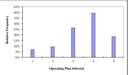
A distribution of operating plan assignments is shown in Figure 5. The relative frequency is biased against high growth scenarios, which do not occur as frequently as other scenarios. Table 7 summarizes results according to different evaluation criteria: ENPV, 5th percentile (P5) value at risk, P95 value at gain, standard deviation, expected initial investment, and expected value of flexibility. Differences between ENPV values obtained with the catalogue and for the baseline system design represents the expected value generated or recognized by

(15)

considerations of flexibility, and using the catalogue technique. It is worth nearly $3.2 million, a 40% improvement compared to the inflexible baseline design with six floors.

0%! 5%! 10%! 15%! 20%! 25%! 30%! 35%! 40%! 45%! 1! 2! 3! 4! 5! R el ati ve F re q u en cy !

Operating Plan Selected!

Figure 5 Relative frequency of each operating plan to each demand scenario Table 7: Multi-criteria evaluation of the design alternatives for each evaluation

technique. All values in $ million

Deterministic Inflexible Catalogue Best?

ENPV 10.6 8.0 11.2 Catalogue

P5 (Value At Risk) N/A -10.8 -4.2 Catalogue

P95 (Value At Gain) N/A 17.7 23.3 Catalogue

Standard Deviation N/A 8.9 8.3 Catalogue

E[Initial Investment] 22.7 22.7 15.2 Catalogue

E[Value of flexibility] - - 3.2

Discussion

The analysis above has two important benefits, observed in the example application. First, it improved the expected lifecycle performance of the system compared to the baseline design obtained via standard practice, by explicitly considering uncertainty in the early conceptual phase. It recognized in the design evaluation process that operators would adapt intelligently to different scenarios. This flexibility has value that needs to be considered explicitly in early design phases, and embedded physically in the design. Otherwise, design alternatives offering less performance may be selected and implemented.

A simple capacity expansion strategy brought significant value improvement in this case, in line with the results reported in the literature on real options analysis and flexibility in engineering design (de Neufville and Scholtes 2011; Nembhard and Aktan 2010; Trigeorgis 1996). Here, value improvements stemmed from the ability to reduce downside losses when demand was not growing fast enough, by reducing initial investment, and by avoiding unnecessary capacity deployment. A flexible design also positioned the system to capture more upside demands, by allowing the system to deploy more parking capacity if needed. This strategy is therefore suited for different risk profiles, as measured by the different metrics (e.g. P5, P95, standard deviation, E[Initial Investment]). The analysis here only considered one flexibility strategy, but more exist (e.g. switch product input/output, defer investment until favorable market conditions, temporarily shut down to reduce downside

(16)

losses, etc.) (Trigeorgis 1996). This observation suggests that there might be even more value available from flexibility in design thinking. Also, this strategy was effective for this system, but every system is different, hence the need to conduct this analysis on a case-by-case basis. Second, the design catalogue technique reduced the number of alternatives to explore, thus addressing the computational issue highlighted in introduction. Only ten iterations were necessary for each scenario to construct the catalogue. This contrasts favorably (i.e. less than 5%) to an exhaustive search requiring the analysis of 216 combinations in this example. This would imply significant time and resources if a more detailed and higher fidelity model was used, such as in the oil and gas case study by Lin et al. (2009), requiring hours and days of computation to analyze one scenario. The analysis presented here is well suited for computational power that is available today. Furthermore, it can be tailored to the engineering system at hand, considering more or less scenarios and operating plans depending on the needs, and available resources.

Limitations and Results Validity

The cause and effect relationships reported here depend evidently on the modeling assumptions. Different values for the design variables, parameters, and decision rules may lead to different conclusions. The results are nonetheless valid and reliable in this case study because the same set of assumptions was used to analyze each scenario and design alternative.

One can assume that the results are generalizable to other engineering systems. The catalogue technique was used to analyze flexibility in real estate development project (Cardin 2007), and in mining operations (Cardin, de Neufville, and Kazakidis 2008), leading to similar conclusions. Although current applications support the claim of generalizability, more applications are needed to further validate the approach.

Another issue is that the set of representative scenarios in step 2 was chosen based on the authors’ inputs. There was nothing special about this particular set. Others could have been chosen, leading to different operating plans, catalogue, and results. There is a need for more research to find a better approach to generating this representative set, to determine useful criteria for terminating the search, and choosing the right number of scenarios. The work done in probability elicitation techniques (Brown 1968; Clemen and Winkler 1999; Morgan and Henrion 1990) represents an interesting area for further exploration.

As mentioned above, only capacity expansion was analyzed in this case study, but more flexibility strategies exist. More work is needed to extend the analysis considering more real options and flexibility alternatives. Also, more work is needed to understand the benefits as compared to full factorial analysis, and other optimizations techniques to explore the design space for each representative scenario.

Lastly, there is no guarantee that the optimal catalogue can be found using this technique. As mentioned by Frey and Wang (Frey and Wang 2006) for a system with n factors of 2-levels, the response can reach up to 80% on average of the optimal solution. This conclusion may not directly apply here since more levels for each factor were explored. On the other hand, the 40% improvement in expected lifecycle performance shows that, as compared to a baseline design, the approach is worthwhile for designers having limited time and computational resources. It produces a good enough solution, and does not require significant analytical and computational resources.

(17)

Conclusions

This paper presented a methodology to improve current systems design and evaluation practice that often relies on simplifying assumptions regarding the main uncertainty drivers affecting lifecycle performance. The proposed approach relies on a set of representative uncertainty scenarios, constructions of a design catalogue, and notions of flexibility in engineering design. Each flexible operating plan is devised to provide an appropriate adaptation plan to each uncertainty scenario. This enables recognizing intelligent managerial decisions in operations, stemming from the flexibility embedded early on in the systems design.

The catalogue approach was applied to the analysis of an example infrastructure system. Considerations of flexibility in the early design showed up to 40% improvements in expected lifecycle performance, as compared to the baseline design developed from standard design and evaluation practice. The analysis required exploring less than 5% of the design space, representing significant economies in terms of time and analytical resources.

More work is needed to fully validate the approach across a broader range of engineering systems. More efforts are needed to develop better approaches for selecting the representative set of uncertainty scenarios. Similarly, computational efficiency needs to be explored more thoroughly in comparison to full factorial analysis, and other optimizations techniques.

Acknowledgments

The authors are thankful for the financial support provided by the National University of Singapore (NUS) Faculty Research Committee via MOE AcRF Tier 1 grants WBS R-266-000-061-133 and R-266-000-067-112, as well as the National Research Foundation through the Singapore-MIT Alliance for Research and Technology Future Urban Mobility research programme via grant WBS R-266-000-069-592. We also acknowledge the financial support provided by the Engineering Systems Division and Center for Real Estate at the Massachusetts Institute of Technology over the period 2005-2011. We are thankful for the intellectual support provided by all ESD, ISE, and SMART colleagues over the period 2005-2012.

(18)

References

Bellman, R. 1952. On the Theory of Dynamic Programming. In Proceedings of the National

Academy of Sciences of the United States of America. Santa Monica, CA, United

States.

Braha, D., A. A. Minai, and Y. Bar-Yam. 2006. Complex Engineered Systems: Science Meets

Technology. Netherlands: Springer.

Brown, B. 1968. Delphi Process: A Methodology Used for the Elicitation of Opinions of Experts. Santa Monica, CA, United States: RAND Corporation.

Cardin, M.-A. 2007. Facing Reality: Design and Management of Flexible Engineering Systems. Master of Science Thesis in Technology and Policy, Engineering Systems Division, Massachusetts Institute of Technology, Cambridge, MA, United States. Cardin, M.-A. 2012. An Organizing Taxonomy of Procedures to Design and Manage

Complex Systems for Uncertainty and Flexibility. In Conference on Complex Systems

Design and Management. Paris, France.

Cardin, M.-A., R. de Neufville, and V. Kazakidis. 2008. A Process to Improve Expected Value in Mining Operations. Mining Technology: IMM Transactions, Section A 117 (2):65-70.

Cardin, M.-A., G. L. Kolfschoten, R. de Neufville, D. D. Frey, O. L. de Weck, and D. M. Geltner. 2012. Empirical Evaluation of Procedures to Generate Flexibility in Engineering Systems and Improve Lifecycle Performance. Research in Engineering

Design, Accepted for publication on 09-28. doi: 10.1007/s00163-012-0145-x

Clemen, R. T., and R. L. Winkler. 1999. Combining Probability Distributions From Experts in Risk Analysis. Risk Analysis 19 (2):187-203.

Copeland, T., and V. Antikarov. 2003. Real Options: A Practitioner’s Guide. New York, NY, United States: Thomson Texere.

Cox, J. C., S. A. Ross, and M. Rubinstein. 1979. Options Pricing: A Simplified Approach.

Journal of Financial Economics 7 (3):229-263.

de Neufville, R., and A. Odoni. 2003. Airport Systems: Planning, Design, and Management. New York, NY, United States: McGraw-Hill Companies Inc.

de Neufville, R., and S. Scholtes. 2011. Flexibility In Engineering Design, Engineering

Systems. Cambridge, MA, United States: MIT Press.

de Neufville, R., S. Scholtes, and T. Wang. 2006. Valuing Options by Spreadsheet: Parking Garage Case Example. ASCE Journal of Infrastructure Systems 12 (2):107-111. de Weck, O. L., D. Roos, and C. L. Magee. 2012. Engineering Systems: Meeting Human

Needs in a Complex Technological World, Engineering Systems Series. Cambridge,

(19)

Dixit, A. K., and R.S. Pindyck. 1994. Investment under Uncertainty. NJ, United States: Princeton University Press.

Eckert, C. M., O. L. de Weck, R. Keller, and P. J. Clarkson. 2009. Engineering Change: Drivers, Sources and Approaches in Industry. In 17th International Conference on

Engineering Design. Stanford, CA, United States.

ESD. 2011. Engineering Systems Division Strategic Report. Cambridge, MA, United States: Massachusetts Institute of Technology.

Frey, D. D., and H. Wang. 2006. Adaptive One-Factor-at-a-Time Experimentation and Expected Value of Improvement. Technometrics 48 (3):418-431.

Gil, N. 2007. On the Value of Project Safeguards: Embedding Real Options in Complex Products and Systems. Research Policy 36:980-999.

Hassan, R., R. de Neufville, and D. McKinnon. 2005. Value-At-Risk Analysis for Real Options in Complex Engineered Systems. In IEEE International Conference on

Systems, Man, and Cybernetics. Hawaii, United States.

Jablonowski, C., C. Wiboonskij-Arphakul, and M Neuhold. 2008. Estimating the Cost of Errors in Estimates Used During Concept Selection. SPE Projects, Facilities, and

Construction 3:1-6.

Jacoby, H., and D. Loucks. 1972. The Combined Use of Optimization and Simulation Models in River Basin Planning. Water Resources Research 8 (6):1401-1414.

Jugulum, R., and D. D. Frey. 2007. Toward a Taxonomy of Concept Designs for Improved Robustness. Journal of Engineering Design 18 (2):139-156.

Lin, J. 2009. Exploring Flexible Strategies in Engineering Systems Using Screening Models – Applications to Offshore Petroleum Projects. Doctoral Dissertation in Engineering Systems, Massachusetts Institute of Technology, Cambridge, MA, United States. Lin, J., O. L. de Weck, R. de Neufville, B. Robinson, and D. MacGowan. 2009. Designing

Capital-Intensive Systems with Architectural and Operational Flexibility Using a Screening Model. In First International Conference in Complex Sciences: Theory and

Applications. Shanghai, China.

Mikaelian, T., D. J. Nightingale, D. H. Rhodes, and D. E. Hastings. 2011. Real Options in Enterprise Architecture: A Holistic Mapping of Mechanisms and Types for Uncertainty Management. IEEE Transactions on Engineering Management 54 (3):457-470.

Morgan, M. G., and M. Henrion. 1990. Uncertainty: A Guide to Dealing with Uncertainty in

Quantitative Risk and Policy Analysis. United Kingdom: Cambridge University Press.

Nembhard, H. B., and M. Aktan. 2010. Real Options in Engineering Design, Operations, and

Management. Boca Raton, FL, United States: Taylor and Francis.

Nembhard, H. B., L. Shi, and M. Aktan. 2005. A Real-Options-Based Analysis for Supply Chain Decisions. IIE Transactions 37:945-956.

(20)

Olewnik, A., and K. Lewis. 2006. A Decision Support Framework for Flexible System Design. Journal of Engineering Design 17 (1):75-97.

Ross, A. 2006. Managing Unarticulated Value: Changeability in Multi-Attribute Tradespace Exploration. Doctoral Dissertation in Engineering Systems, Massachusetts Institute of Technology, Cambridge, MA, United States.

Rothwell, G. 2006. A Real Options Approach to Evaluating New Nuclear Power Plants.

Energy Journal 27:37-54.

Steel, K. D. 2008. Energy System Development in Africa: The Case of Grid and Off-Grid Power in Kenya. Doctoral Dissertation in Engineering Systems, Massachusetts Institute of Technology, Cambridge, MA, United States.

Sterman, J. D. 2000. Business Dynamics: Systems Thinking and Modeling for a Complex

World. Boston, MA, United States: McGraw-Hill/Irwin.

Tomiyama, T., P. Gu, Y. Jin, D. Lutters, Ch. Kind, and F. Kimura. 2009. Design Methodologies: Industrial and Educational Applications. CIRP Annals –

Manufacturing Technology 58:543-565.

Trigeorgis, L. 1996. Real Options. Cambridge, MA, United States: MIT Press.

Wang, T. 2005. Real Options in Projects and Systems Design – Identification of Options and Solutions for Path Dependency. Doctoral Dissertation in Engineering Systems, Massachusetts Institute of Technology, Cambridge, MA, United States.

Wang, T., and R. de Neufville. 2005. Real Options ‘In’ Projects. In Real Options Conference. Paris, France.

Yang, Y. 2009. A Screening Model to Explore Planning Decisions in Automotive Manufacturing Systems Under Demand Uncertainty. Doctoral Dissertation in Engineering Systems, Massachusetts Institute of Technology, Cambridge, MA, United States.

Zhang, S. X., and V. Babovic. 2012. A Real Options Approach to the Design and Architecture of Water Supply Systems Using Innovative Water Technologies Under Uncertainty. Journal of Hydrodynamics 14 (1):13-29.

(21)

Appendix

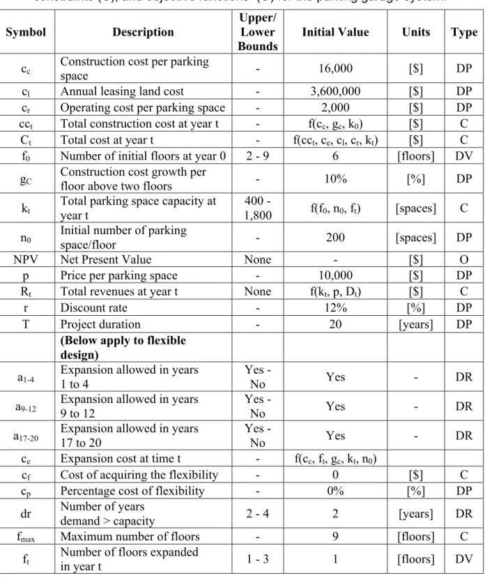
Table 8 Master table summarizing design variables (DV), parameters (DP), constraints (C), and objective functions (O) for the parking garage system.

Symbol Description

Upper/ Lower Bounds

Initial Value Units Type

cc Construction cost per parking _space - 16,000 [$] DP

cl Annual leasing land cost - 3,600,000 [$] DP

cr Operating cost per parking space - 2,000 [$] DP

cct Total construction cost at year t - f(cc, gc, k0) [$] C

Ct Total cost at year t - f(cct, ce, cl, cr, kt) [$] C

f0 Number of initial floors at year 0 2 - 9 6 [floors] DV

gC Construction cost growth per _{floor above two floors} - 10% [%] DP

kt Total parking space capacity at _{year t} _1,800400 - f(f0, n0, ft) [spaces] C

n0 Initial number of parking _space/floor - 200 [spaces] DP

NPV Net Present Value None - [$] O

p Price per parking space - 10,000 [$] DP

Rt Total revenues at year t None f(kt, p, Dt) [$] C

r Discount rate - 12% [%] DP

T Project duration - 20 [years] DP

(Below apply to flexible design)

a1-4 Expansion allowed in years _{1 to 4} Yes - _No Yes - DR

ce Expansion cost at time t - f(cc, ft, gc, kt, n0)

cf Cost of acquiring the flexibility - 0 [$] C

cp Percentage cost of flexibility - 0% [%] DP

dr Number of years

demand > capacity 2 - 4 2 [years] DR

fmax Maximum number of floors - 9 [floors] C

(22)

600! 800! 1000! 1200! 1400! 1600! 1800! 1! 2! 3! 4! 5! 6! 7! 8! 9! 10! 11! 12! 13! 14! 15! 16! 17! 18! 19! 20! D eman d (s p ac es )! Time (years)!

Original demand projection! Demand scenario 1! Demand scenario 2!

Demand scenario 3! Demand scenario 4! Demand scenario 5!

Figure 6 Set of representative demand scenarios based on the exponential demand model with β = 0.990, 0.500, 0.250, 0.125, and 0.050.

(23)

Biographies

Michel-Alexandre CARDIN is Assistant Professor of Industrial and Systems Engineering at

the National University of Singapore. His research focuses on the development and evaluation of practical procedures to support the design of engineering systems for flexibility. He holds a Ph.D. and Master of Science in Engineering Systems from MIT, a Master of Applied Sciences in Aerospace Engineering from the University of Toronto, an Honours Bachelor's degree in Physics from McGill University, and is a graduate from the Space Science Program at the International Space University. He currently serves on the Editorial Review Board of the peer-reviewed journal IEEE Transactions on Engineering Management, and is a member of the INCOSE Singapore Chapter.

Richard DE NEUFVILLE is Professor of Engineering Systems and of Civil and

Environmental Engineering at MIT. His current research and teaching focuses on improving performance by inserting flexibility into the design of technological systems. He is the author of many textbooks on systems analysis, planning and design. His latest, Flexibility in

Engineering Design, co-authored with Stefan Scholtes at the University of Cambridge, was

published in 2011 in the MIT Series on Engineering Systems. He has a Ph.D. from MIT and a Dr. h.c. from Delft University of Technology. He has been associated with the development of major infrastructure projects on all continents (except Antarctica). He is now closely associated with the development of the new Singapore University of Technology and Design.