Hydrogeological characterization of karst aquifers in Switzerland using a pragmatic approach

Faculté des Sciences Rue Emile Argand 11

Swiss Institute for Speleology

and Karst Studies

PhD Thesis submitted to the Faculty of Sciences

Centre for Hydrogeology and Geothermics (CHYN)

University of Neuchâtel

For the degree of PhD

by

Arnauld Malard

Accepted by the dissertation committee:

Prof. Pierre-Yves Jeannin, University of Neuchâtel (CHYN), ISSKA, thesis director

Prof. Daniel Hunkeler, University of Neuchâtel (CHYN)

Prof. Benoît Valley, University of Neuchâtel (CHYN)

Dr. Nathalie Dörfliger, BRGM Orléans, France

Prof. Zoran Stevanovic, University of Belgrade, Serbia

Defended on May 16

, 2018

Hydrogeological characterization of karst aquifers in

Switzerland using a pragmatic approach

Tél : + 41 (0)32 718 21 00 E-mail : secretariat.sciences@unine.ch

IMPRIMATUR POUR THESE DE DOCTORAT

La Faculté des sciences de l'Université de Neuchâtel

autorise l'impression de la présente thèse soutenue par

Monsieur Arnauld MALARD

Titre:

“

Hydrogeological characterization of karst

aquifers in Switzerland using a pragmatic

approach

”

sur le rapport des membres du jury composé comme suit:

•

Prof. Pierre-Yves Jeannin, directeur de thèse, UniNE

•

Prof. Benoît Valley, UniNE

•

Prof. Daniel Hunkeler, UniNE

•

Dr Nathalie Dörfliger, BRGM, Orléans, France

•

Prof Zoran Stevanovic, Université de Belgrade, Serbie

Acknowledgments

The work was realized under the authority of Pierre-Yves Jeannin, director of SISKA: Swiss Institute for Speleology and Karst Studies, La Chaux-de-Fonds, 2300 Switzerland (www.isska.ch). In parallel to this dissertation, several collaborators of SISKA were involved in the Swisskarst project. They bring their personal input for the development of the KARSYS approach and their contribution for the work of aquifers documentation.

The dissertation has been accompanied by Daniel Hunkeler, director of the Centre for Hydrology of the University of Neuchâtel (CHYN).

This dissertation has been realized in the frame of the Swiss National Research Program 61, supported by the Swiss National Foundation for Sciences. Additional supports have been also provided by the Federal Office for Environment (Section Hydrogeology) and several cantons: BE, JU, VD, SG, FR and VS for applying KARSYS on their territory. Finally, the application of KARSYS in Slovenia was made possible thanks to the Swiss Contribution Grant to the enlarged UE.

I would like to express my personal thanks to the following persons:

- Jonathan Vouillamoz, Eric Weber, Silvia Schmassmann†, Urs Eichenberger, Constanze Bonardo and Demian Rickerl, SISKA, for their implication in the Swisskarst project. Different trainees were also involved, essentially for data compilation since the project started in 2010.

- Michael Sinreich from the Federal Office for Environment for having supported many aspects of the Swisskarst project and for its contribution as co-author for two relevant papers.

- Frederic Jordan and Murielle Thomet, e-dric for having provided free licenses of RS3.0 as well as numerous advices on the use of the software.

- Janez Turk (ex. Slovenian Karst Research Institute) and Daniel Ballesteros (University of Oviedo, Spain) for having experienced the KARSYS approach on their sites, respectively in Slovenia and in Spain. They bring their personal input and critics on the approach and they promote KARSYS throughout various publications

I thank also the following companies that provide data and information in the frame of the Swisskarst project: RWB, MFR (Marc Hessenhauer), Kellerhals & Haefeli, as well as various researchers who provide interesting inputs or advices: Miriam Coenders-Gerrits (Delft University of Technology), Andres Wildberger (Büro von Moos).

Foreword

This dissertation has been performed in the frame of the Swisskarst project, part of the National Research Program 61 (Jan. 2010 - Dec. 2013) related to the “Sustainable Water Management in Switzerland”. The project was supported by the Swiss National Research Foundation. Objectives of the project were to establish and improve a pragmatic approach (KARSYS) to document the hydrological functioning of karst systems over the territory in order to provide a support to improve their management. This covers a large range of fields such as water supply, civil engineering, renewable energies, natural hazards, etc.

The Swisskarst project started in early 2010. A first PhD student was engaged but he left the position in April 2010. A second student has been engaged but she also left in April 2011. In total these two PhD students used up 11 months of salary and provided only a very restricted number of useful ideas and work for the project. Arnauld Malard was finaly committed in June 2011 and a request for additional financial was submitted in October 2011 in order to complete the financing of this third PhD-student. Then the project really started only about one year later the beginning of the NRP61.

The Swisskarst project has received further support from federal offices, cantons and communities which bring their respective expectations. All along these four years, the approach has been applied on the following cantons: Vaud, Bern, St-Gall, Fribourg and punctually Neuchâtel, Jura, Schwyz, Graubünden but also for private companies (i.e. CSD, BG ingénieur conseil, Buchs & Plumey, e-dric, SEFA…). Thanks to various collaborations with institutions abroad, the approach was also applied in Slovenia (2012), in Spain (2013) and later in Ireland and France. Over these 4 years, the KARSYS approach has been expanded on nearly 1/3 of the Swiss territory and more than hundred karst systems have been documented.

ISSKA - SISKA

The Swiss Institute for Speleology and Karst Studies is active on various karst-related fields: fundamental and

applied scientific research (geology, hydrogeology, cave climate, speleology, and paleontology), teaching, protection of the karst heritage, safety measures, and national speleological documentation. The institute has

been launched in 1999 as a non-profitable foundation - two years after the 12th _{International Congress of}

Speleology.

The office is located at La Chaux-de-Fonds (NE).

SISKA mainly works for cantonal authorities, communities, water authorities, engineers and consulting firms. It frequently collaborates with universities, high-schools and geological private companies, in Switzerland but also abroad.

The staff entails 11 permanent collaborators (hydrogeologist, geologist, biologist, administration and graphic designer) and temporary collaborators: trainees, voluntaries from the Civil Service, etc.

Abstract / Résumé

[EN] Recent studies reveal that karst aquifers represent a significant part of the Swiss groundwater reserve

(120 km3_{) and resource (8.4 km}3_{/year), although they only extend over 20% of the territory. On the one}

hand, high infiltration rates and large permeabilities of karstified rocks make karst aquifers highly interesting for water management. On the other hand, karst groundwater flow-systems are characterized by a highly heterogeneous structure including quick- and slow-flow components (conduit network, phreatic and epikarst storage) which lead to important hydrodynamic variabilities and complex flow dynamics which cannot be solved by the mean of standard hydrogeological tools. Finally, karst aquifers are also highly vulnerable to contamination and require specific attention for protection. Consequently, in spite of interesting groundwater resources, karst aquifers are often disregarded, flow-dynamics are poorly known and groundwater management is far from being optimal.

These are the reasons which motivated SISKA to submit the Swisskarst project as part of the Swiss National Research Program 61 dedicated to sustainable water management in Switzerland (Jan. 2010 – Dec. 2013). The motivation of the Swisskarst project was to develop a 3D conceptualization approach (KARSYS) for improving the hydrogeological characterization of karst aquifers. This dissertation is directly related to the Swisskarst project and to the KARSYS approach.

All along the project, the existing form of the KARSYS approach has been tested on various sites in Switzerland and abroad in order (i) to test the applicability on real sites, (ii) to formalize methodological steps and (iii) to improve standard operations. Compared to the initial form of KARSYS (as published in 2013), semi-automatized procedures have been developed for generating conduit network and for delineating the systems catchment over the ground surface. Applications of KARSYS to numerous case studies showed that the approach reveals extremely efficient for documenting epigenic karst aquifers where karst processes are in equilibrium with hydrological base level, where contrasts of lithologies make it possible to identify karstified rocks from non-karstified rocks and where phreatic zones are of moderate extension or compartmentalized into several distinct units. For pure confined aquifers or where lithological contrasts make difficult to distinguish karstified from non-karstified rocks, KARSYS remains applicable but less fruitful. Main limitations in the applicability of KARSYS concern the precision of geological data and hydrological indications regarding karst springs (activity, mean discharge, etc.).

As KARSYS is a conceptual approach, numerical approaches of simulation have been developed as extensions. Two types of simulation models have been designed for groundwater recharge: one for alpine regions where recharge is dominated by relief-contrasts, snow and glacier melts and one other for low-land regions where recharge are dominated by vegetation and soils/epikarst processes. Applications of these models make it possible to distinguish all the components of the recharge processes (precipitation, RET, etc., with the exception of the condensation) in the different compartments of the aquifers (storage in soils, epikarst, low permeable volumes, etc.). In addition to these recharge model, a hydraulic model for

simulating flows in the conduit network has been developed. This model uses the generated conduit network and the simulated recharge as inputs to reproduce the discharge for each outlets of the flow-system. Applications of these models with a constant interaction with the 3D conceptual model of the karst aquifers make it possible to infer additional properties of flow-systems (perched conduits, thresholds, etc.). These models may now address various issues in karst hydrology (storage, impacts of construction, flood hazards, etc.).

Another extension has been developed in the form of guidelines for mapping hydrogeological information resulting from the application of KARSYS. These guidelines promote three types of karst hydrogeological maps depending on the scale and on the issues: the karst groundwater map, the karst aquifer map and the karst flow-system map.

Finally, this project was also the opportunity to address general questions on karst groundwater at Swiss scale: the annual recharge, the minimal low-flow storage and the seasonal storage and the expected evolution of groundwater resources with the climate changes. These works made it possible to provide insights, key-values or recommendations regarding the current dynamics of karst aquifers and their expected evolution in the coming decades. They will contribute to support decision regarding future strategies for karst groundwater management.

Approaches and extensions which have been developed in this dissertation contribute to improve knowledge on karst aquifers in the scope of improving the sustainable management of groundwater in Switzerland.

Key words: karst hydrology, karst hydraulic, conceptual model, conduits generation, flow simulation

[FR] Des études récentes révèlent que les aquifères karstiques représentent une part importante des

réserves en eau souterraine de la suisse (120 km3) et des ressources renouvelables (8,4 km3/an), bien qu'ils

ne s'étendent que sur 20% du territoire. D'une part, les taux d'infiltration élevés et les grandes perméabilités des roches karstifiées rendent les aquifères karstiques très intéressants pour la gestion de l'eau. D'autre part, les systèmes d'écoulement karstiques sont caractérisés par une structure très hétérogène à composantes d’écoulement rapides et lentes (réseau de conduits, stockage phréatique et épikarst) qui conduisent à d'importantes variations hydrodynamiques et à des dynamiques d'écoulement complexes qui ne peuvent être résolues à l'aide d'outils hydrogéologiques standard. Enfin, les aquifères karstiques sont également très vulnérables à la contamination et nécessitent une attention particulière pour leur protection. Par conséquent, malgré des ressources en eaux souterraines intéressantes, les aquifères karstiques sont souvent ignorés, la dynamique de l'écoulement est mal connue et la gestion des eaux souterraines est loin d'être optimale.

C'est pour ces raisons que l'ISSKA a décidé de présenter le projet Swisskarst dans le cadre du Programme National Suisse de Recherche 61 consacré à la gestion durable de l'eau en Suisse (janvier 2010 - décembre 2013). La motivation du projet Swisskarst était de développer une approche conceptuelle 3D (KARSYS) pour améliorer la caractérisation hydrogéologique des aquifères karstiques. Cette thèse est directement liée au projet Swisskarst et à l'approche KARSYS.

Tout au long du projet, la forme existante de l'approche KARSYS a été testée sur différents sites en Suisse et à l'étranger afin (i) de tester l'applicabilité sur des sites réels, (ii) de formaliser les étapes méthodologiques et (iii) d'améliorer les opérations standards. Par rapport à la forme initiale de KARSYS (telle que publiée en 2013), des procédures semi-automatisées ont été développées pour générer un réseau de conduits et pour délimiter les bassins d’alimentation en surface. Les applications de KARSYS à de nombreuses études de cas ont montré que l'approche se révèle extrêmement efficace pour documenter les aquifères karstiques épigéniques où les processus karstiques sont en équilibre avec le niveau de base hydrologique, où les contrastes des lithologies permettent d'identifier les roches karstifiées à partir de roches non karstifiées et

où les zones phréatiques sont d'extension modérée ou compartimentées en plusieurs unités distinctes. En ce qui concerne les aquifères purement confinés ou lorsque les contrastes lithologiques rendent difficile la distinction entre les roches karstifiées et les roches non karstifiées, l’approche KARSYS reste applicable mais moins performante. Les principales limites à l'applicabilité de KARSYS concernent la précision des données géologiques et des indications hydrologiques concernant les sources karstiques (activité, débit moyen, etc.). Comme KARSYS est une approche conceptuelle, des approches numériques de simulation ont été développées en tant qu'extensions. Deux types de modèles de simulation ont été conçus pour la recharge des eaux souterraines : l'un pour les régions alpines où la recharge est dominée par les contrastes de relief, la fonte des neiges et des glaciers et l'autre pour les régions basses où la recharge est dominée par la végétation et les processus sol/épikarst. Les applications de ces modèles permettent de distinguer toutes les composantes des processus de recharge (précipitations, RET, etc., à l'exception de la condensation) dans les différents compartiments des aquifères (stockage dans les sols, épikarst, volumes faiblement perméables, etc.). En plus de ces modèles de recharge, un modèle hydraulique de simulation des débits dans le réseau de conduits a été développé. Ce modèle utilise le réseau de conduits généré et la recharge simulée comme entrées pour reproduire la décharge à chaque exutoire du système d'écoulement. Les applications de ces modèles en interaction constante avec le modèle conceptuel 3D permettent de déduire des propriétés supplémentaires des systèmes d'écoulement (conduits perchés, seuils, etc.). Ces modèles peuvent maintenant aborder diverses questions relatives à l'hydrologie karstique (stockage, impacts de la construction, risques d'inondation, etc.).

Une autre extension a été développée sous la forme de lignes directrices pour la cartographie de l'information hydrogéologique résultant de l'application de KARSYS. Ces lignes directrices favorisent trois types de cartes hydrogéologiques karstiques selon l'échelle et les enjeux : la carte des eaux souterraines karstiques, la carte des aquifères karstiques et la carte du système d'écoulement karstique.

Enfin, ce projet a également été l'occasion d'aborder des questions générales sur les eaux souterraines des aquifères karstiques à l'échelle suisse : la recharge annuelle, le stockage minimal à faible débit et le stockage saisonnier et l'évolution attendue des ressources en eaux souterraines avec les changements climatiques. Ces travaux ont permis de fournir des aperçus, des valeurs clés ou des recommandations concernant la dynamique actuelle des eaux souterraines et leur évolution prévue dans les décennies à venir. Ils contribueront à appuyer les décisions concernant les stratégies futures de gestion des eaux souterraines karstiques.

Les approches et extensions développées dans cette thèse contribuent à améliorer les connaissances sur les aquifères karstiques dans la perspective d’une gestion durable des ressources.

Mots clefs : hydrologie karstique, hydraulique karstique, modèle conceptuel, génération de réseaux de conduits, simulation d’écoulement

–TABLE OF CONTENTS Acknowledgments ... 1 Foreword... 2 Abstract / Résumé ... 3 Introduction ... 23 1. 1.1. Generalities and background ... 23

1.1.1. The Swisskarst project ... 23

1.1.2. General issues related to karst environments ... 23

1.1.3. Main characteristics of karst in Switzerland ... 24

1.2. Problem summary... 27

1.3. Objectives of the thesis ... 27

1.4. Structure of the chapters ... 28

Groundwater in karst ... 31 2. 2.1. Karst aquifer ... 31 2.1.1. Definition ... 31 2.1.2. Distribution ... 32 2.1.3. Characteristics ... 33 2.2. Karst flow-system ... 38 2.2.1. Recharge zone ... 38 2.2.2. Drainage zone ... 39 2.2.1. Discharge zone ... 47 2.3. Hydrology ... 48 2.3.1. Recharge ... 49 2.3.2. Storage ... 58 2.4. Conclusion ... 61

Main issues in karst and related users ... 63

3. 3.1. Issues ... 63

3.1.1. Drinking water supply ... 63

3.1.2. Natural hazards ... 68

3.1.3. Renewable energies in karst: geothermal and hydropower ... 74

3.1.4. Civil engineering in karst environment... 82

3.1.5. Clear (and waste) water evacuation – artificial injection ... 85

3.1.6. Ecological services ... 86

3.1.7. Heritage and Tourism ... 86

3.3. Conclusion: making karst more accessible for users? ... 91

Approaches to the hydrogeological characterization of karst ... 93

4. 4.1. Characterization approaches ... 93 4.1.1. Definition ... 93 4.1.2. Outputs ... 97 4.2. Application workflow ... 97 4.2.1. Karst contexts ... 99

4.2.2. Models of general principles ... 99

4.2.3. Investigation methods ... 100

4.2.4. Tools ... 103

4.3. Hydrogeological mapping in karst ... 104

4.3.1. Review of existing mapping processes ... 104

4.3.2. Limitations of existing mapping approaches ... 106

4.3.3. Karst hydrogeological maps based on KARSYS ... 106

4.4. Conduits network generation in a karst aquifer ... 107

4.4.1. Issues in conduits generation ... 108

4.4.2. Principles governing the development of karst conduits ... 108

4.4.3. Existing approaches for the generation of conduit networks (review from the literature) 109 4.4.4. Discussion of existing approaches for conduits generation ... 112

4.5. Flow simulation in karst ... 113

4.5.1. Generalities ... 113

4.5.2. Main aspects of existing approaches for hydrological modelling ... 114

4.6. Mismatches between existing approaches and needs for the practice ... 124

The KARSYS approach ... 125

5. 5.1. Introduction ... 125

5.2. KARSYS Original 3D ... 126

5.2.1. Steps in the application of KARSYS Original 3D ... 127

5.2.2. Outputs ... 140

5.2.3. Advantages of KARSYS ... 140

5.2.4. Limitations ... 141

5.2.5. Conditions for application ... 142

5.2.6. Validation procedures ... 146

5.3. Conclusion ... 150

KARSYS extensions ... 151 6.

6.1. Summary ... 151

6.2. Catchment delineation and conduit modelling based on the KARSYS approach (peer-reviewed paper, Hydrogeology journal 2015) ... 152

6.3. Hydrological and hydraulic simulations in karst ... 170

6.3.1. Introduction ... 170

6.3.2. Test-site description ... 172

6.3.3. Recharge simulations ... 184

6.3.4. Hydraulic simulations ... 206

6.3.5. Discussion / conclusion on flow simulations in karst ... 218

Karst groundwater resources in Switzerland, evolution with climate changes and 7. perspectives for water management ... 227

7.1. Annual resources in karst aquifers ... 227

7.2. Evolution of water resources in karst aquifers with climate changes ... 242

7.2.1. Effects on groundwater recharge ... 242

7.2.2. Effect of increasing extremes ... 243

7.2.3. Effects on water quality ... 245

7.2.4. Effects on soil and vegetation ... 246

7.3. Perspectives for karst water management ... 246

7.3.1. Specific management rules for karst environments ... 246

7.3.2. Survey and investigation ... 247

7.3.3. Direct water exploitation ... 247

7.3.4. Indirect exploitation ... 248

Conclusion ... 249

8. 8.1. Improvements of KARSYS and extensions ... 250

8.2. Swiss karst aquifers, key-values of actual dynamics and expected evolution ... ... 252

8.3. Outlook: Visual KARSYS ... 253

Bibliography ... 255

9. Appendices ... 277

10. 10.1. Appendix 1: Swisskarst, a project of the 61st National Research Program ... 279

10.1.1. The 61th National Research Program ... 279

10.1.2. The Swisskarst project... 279

10.2. Appendix 2: review of classifications of porosity in carbonate and karst aquifers ... 287 10.3. Appendix 3: Malard et al. 2014 - Assessing the Contribution of Karst to Flood Peaks of the Suze River, Potentially Affecting the City of Bienne (Switzerland) ... ... 291

10.4. Appendix 4: additional information on karst groundwater quality ... 299

10.4.1. Groundwater temperature ... 299

10.4.2. Suspended sediments ... 302

10.4.3. Inorganic contaminants ... 302

10.4.4. Microbes and Pathogens ... 303

10.4.5. Anthropogenic Organic Compounds ... 305

10.4.6. Evolution over the last decades ... 306

10.5. Appendix 5: examples of karst-related problems for tunnels in Switzerland ... ... 309

10.6. Appendix 6: Malard et al. 2014 - Impact of a Tunnel on a Karst Aquifer: Application on the Brunnmühle Springs (Bernese Jura, Switzerland) ... 311

10.7. Appendix 7: Malard et al. 2012 - toward a sustainable management of karst water in Switzerland. Application to the Bernese Jura ... 319

10.8. Appendix 8: Additional information on the limitations of the KARSYS approach ... 325

10.9. Appendix 9: Malard et al. 2016 - Praxisorientierter Ansatz zur kartographischen Darstellung vonKarst-Grundwasserressourcen... 333

10.10. Appendix 10: Malard et al. 2014 - Assessing Karst Aquifers in Switzerland: The 2010/2013 Swisskarst Project ... 347

10.11. Appendix 11: Efficiency criteria for models calibration and validation ... 353

10.12. Appendix 12: RS3.0 Simulation test ... 355

10.12.1. Design of the recharge simulation model ... 355

10.12.2. Calibration ... 355

10.12.3. Simulation 2007 ... 357

10.13. Appendix 13: Selection of appropriate meteorological stations in Ajoie (JU) for being used in the recharge models ... 359

10.14. Appendix 14: Simplified hydraulic model ... 361

10.14.1. Model design ... 361

10.14.2. Calibration and validation ... 362

10.14.3. Simulation of the flood event from August 2007 ... 365

–FIGURES

Figure 1—1. Distribution of the outcropped carbonate formations over the Swiss territory which may be potentially karstified and location of caves dense-areas (from 10 to 20 known entrances per km2 _{for the}

most investigated sites). Geological data comes from Swisstopo. _________________________________ 24 Figure 1—2. Swiss documented areas from a karst-hydrogeological or morphological point of view prior to the Swisskarst project. Black breakdowns refer to Swiss official hydrogeological maps (1/100’000, Swisstopo) _____________________________________________________________________________ 25 Figure 1—3. Schematic sketch of various karst environments in Switzerland _________________________ 26 Figure 1—4. Objectives and guiding thread of the dissertation; each block refers to chapters that are developed hereafter _____________________________________________________________________ 29 Figure 2—1. Distribution of carbonate rocks over the World (SGGES, University of Auckland, New Zealand); numerous populated and « arid » zones (Mediterranean, Persian Gulf, Central America, etc.) are located in karst area. Two types of aquifers are here distinguished; (i) outcropping carbonate rocks (black) and (ii) “deep” or overlaid carbonate rocks (grey). Most of these carbonate rocks are supposed to be karstified. _ 32 Figure 2—2. Schematic vertical structuration of epigenic karst aquifers (from Doerfliger [1997]). From top to bottom, karst aquifers are sub-divided into four main zones: Soil, Epikarst, Unsaturated zone and the saturated (phreatic zone). The unsaturated zone may be divided in two zones: the vadose which never floods and the epiphreatic zone which periodically floods ________________________________________ 33 Figure 2—3. Schematic profile of the soil and of the epikarst in karst terrane ________________________ 34 Figure 2—4. Vertical zones in a karst aquifer and associated ranges of effective porosity (completed from Filipponi et al. [2012]) ____________________________________________________________________ 37 Figure 2—5. Schematic cross-section of a karst flow-system (alpine or jurassian environment); imp.: aquifer basement, Fvv: vertical vadose flows, Fvc: basement-controlled vadose flows, Fplf: phreatic

low-flows, Fphf: epiphreatic flows (figure from Malard [2013]). ______________________________________ 40

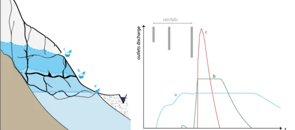
Figure 2—6. Schematic profile of the epiphreatic zone of a karst aquifer (left) and corresponding hydrographs (right). Recharge intensity, interconnection, elevation, volume and discharge capacity of the epiphreatic conduits are the main controlling factors of the hydraulic gradient evolution. While the hydraulic gradient rises and floods the epiphreatic zone (left), one part of the coming water is successively drained by overflow conduits, leading to a multi-component signal at the respective springs (right), while the other part may be stored and later released (figure from Malard et al. [2014a]) __________________ 46 Figure 2—7. Karst springs are mainly of three types depending on the context of emergence: free draining springs, dammed springs and confined springs (figure from Ford and Williams [2007]). Whatever the context, if the epiphreatic zone shows significant fluctuations, one or several overflow spring(s) may exist upstream from the permanent one(s). _______________________________________________________ 48 Figure 2—8. Schematic organization of the karst groundwater recharge components; each component is

described here-after _____________________________________________________________________ 49 Figure 2—9. Structuration of interception reservoir; Hmax inter fixes the storage capacity which evolves with

the seasons, Hinter is the stored water, Ev the losses by evaporation and iover the part of water infiltrating

through the soils. ________________________________________________________________________ 52 Figure 2—10. Seasonal evolution of the storage capacity for a beech forest (above: only the canopy, center: forest floor, below: canopy + forest floor) in Luxembourg (measurements from Gerrits et al.

[2010]). Regarding the canopy, the storage capacity varies from 0.1 mm in February to 1.2 mm in June. As the falling season appears, the storage capacity (i.e. the interception power) significantly decreases. Regarding the forest floor, the maximum is reached in fall. ______________________________________ 54 Figure 2—11. Example of relation between the vegetation Leaf Area Index (LAI) and the coefficient of

evaporation for temperate climate (Specht and Specht [1989]); the map provides an overview of the LAI mean distribution over the world. ___________________________________________________________ 55 Figure 2—12. General model of flows through soils and epikarst; depending on the saturation of the reservoir, a part of the flows may by-pass the soil or the epikarst and reach the conduit network. Water stored in these reservoirs contributes to evapotranspiration ET. ET depends on PET, EV from the

interception and H, the water stored in soils and epikarst. _______________________________________ 56 Figure 2—13. Combined effects of the drainage capacity, the aquifer thickness and the effective porosity on the storage capacity of the aquifer _______________________________________________________ 58 Figure 3—1. Information related to the location of the phreatic (saturated) zone and of the expected horizons of high probability of karst is essential to succeed in drilling wells. _________________________ 65 Figure 3—2. Above: example of karst collapse occurring in a street in La Chaux-de-Fonds (NE); apparition of these collapses in ultra-urban zones is intensified by breakdowns or leakages of drinking- or storm-water pipes. Middle: sudden collapse in sub-urban zone; apparition of this sinkhole close to the house may be enhanced by the storm-water infiltration device. Below: collapse in rural zone; this is related to the fluctuations of the groundwater table, which frequently reaches the level of the road basement. _______ 70 Figure 3—3. High-flow events in karst environments may provoke hazards at land surface (Jeannin [2014]). Landslides/rockslides, subsidence/collapses and sinkholes formation occur more frequently in the range of the karst groundwater oscillations. Debris flows and floods usually occur in areas downstream from perennial and temporary karst springs or in the area of diffuse groundwater exfiltration. Due to underground thresholds between systems A and B, aquifer B may suddenly receive a considerable amount of water coming from aquifer A for high-flows. Intensity of the flood in the system B suddenly increases and may provoke associated hazards (mudflows, landslides, etc.). ________________________________ 72 Figure 3—4. Considering that conduits are efficient for heat drainage, their density and distribution within the massif and the groundwater flux impact the ascending geothermal heat flux. At some locations, aquifers of type (a.) reveal favorable for the implantation of geothermal probes while karst systems of

type (b.) may offer more interesting conditions for springs heat exploitation as most of the geothermal flux

is absorbed by the flows and carried out at the spring. __________________________________________ 76 Figure 3—5. Open-loop systems in karst aquifer enhance sediments mobilization or dissolution and may provoke land-subsidence (Cooper et al. [2011]). These mechanisms frequently occur in confined /semi-confined aquifers. This lead UK authorities to develop a decision support tool (GeoSure) which gives

indication on areas to karst collapses susceptibility and recommends the type of devices to implant (open or close loop). ___________________________________________________________________________ 77 Figure 3—6. Various scenarios of geothermal probes in karst; A: although the probe may reveal efficient,

this scenario may impact the groundwater quality as the probe connects both aquifers. In theory, usual regulations strictly prohibit this scenario but implementations in practice are difficult as they require a consistent knowledge on the structuration of the aquifer with the depth; B: although the probe is located

in a non karst area, it intersects two superimposed aquifer and may connect them. This configuration may reveal efficient for heat production if the probe intersects the conduits but it may also impact the groundwater. Usual regulations should prohibit this scenario – at least if the geological background is

sufficient to assess the extension of the karst aquifer below the non-karstic formations… C: the probe is

located in a non-karst area even though it intersects the underlying karst aquifer. This scenario a priori does not present hazard for the karst groundwater – at least until the karst aquifer is non artesian; D: the

probe is drilled in karst area and it reaches the saturated part of the karst aquifer. This configuration is not supposed to be problematic for the groundwater as long as it is located far from the supplied spring. However, some cantons strictly prohibit the probes to penetrate in the phreatic zone. In such conditions the efficiency of the probe is supposed to be moderate; E: the probe is located in karst area but it does not

penetrate the phreatic zone. Although this scenario is not supposed to be problematic for the groundwater, the efficiency of the probe lying exclusively in the unsaturated zone is supposed to be moderate and to spatially evolve; F: the probe is drilled in karst area, close to the supplied karst spring. As

a potential impact on the groundwater does exist (chemical contamination, etc.), this scenario is usually prohibited, G: in this scenario, the probe is drilled in karst area and it intersects two superimposed aquifer.

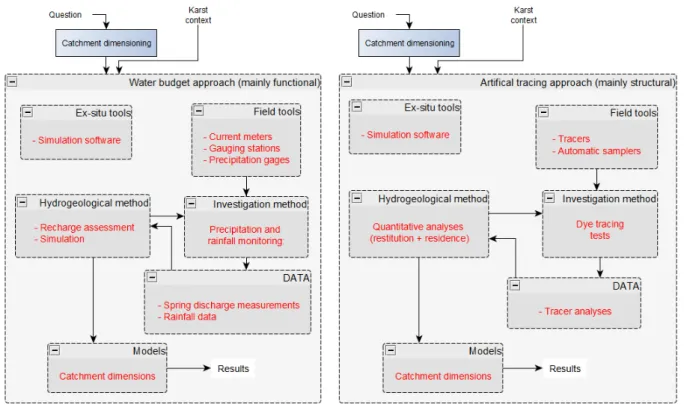
As the lower confined aquifer is here artesian, a real risk of artesian by-pass has to be considered. Even if the probe may reveal “highly” efficient, it should be prohibited in such a situation. ___________________ 77 Figure 3—7. Different capture techniques for hydropower production in karst aquifers (Jeannin [2014]) __ 81 Figure 4—1. Organization of the characterization approaches in karst _____________________________ 94 Figure 4—2. Systematic workflow of a characterization approach to address a karst-related question. ___ 98 Figure 4—3. Two examples of application of characterization approach to address the question of catchment dimensioning in karst area; left: by applying the water budget approach (= functional approach) and right: by applying the artificial tracing approach (= structural approach) _______________ 99 Figure 4—4. The applied question should be first translated into specific hydrogeological question(s) before applying investigation method(s) __________________________________________________________ 100 Figure 4—5. Theoretical way (A) versus “in-practice” way (B) when applying the approach; due to financial

limits and existing data, interpretation methods are usually imposed. In a theoretical way, the interpretation methods are initially selected depending on the questions and they control the investigations to be performed. ___________________________________________________________ 101 Figure 4—6. Example of application for an approach in theoretical way (A) and “in-practice” way (B) for a

given question which has been translated into specific hydrogeological question(s). In case (A), the

hydrogeological question is inferred from the given question and guides the investigation method(s) to be applied. In case (B), existing data (here water isotopes obtained from previous campaigns of analyses) bias

the hydrogeological questions which partly answer the original issue. ____________________________ 101 Figure 4—7. Overview of the existing approaches for conduits generation in karst. Approaches combine temporal and/or spatial data to interpret the geometry of the conduit network. ____________________ 109 Figure 4—8. Hydrological models in karst have to address one or several of these three main applications: (A) system recharge assessment, (B) system discharge assessment and (C) outlets discharge assessment 114 Figure 4—9. Classification of hydrological simulation approaches in karst _________________________ 115 Figure 4—10. Hydrological and hydrogeological simulation models in karst; synthesis _______________ 122 Figure 5—1. Workflow of KARSYS Original 3D (modified from Jeannin et al. [2013])__________________ 127 Figure 5—2. Example of hydrostratigraphic model for the Upper Jurassic limestone in the Swiss Jura (Malm); principles and criteria for the distinction between karst aquifers and karst aquicludes are presented here-after. ____________________________________________________________________ 128

Figure 5—3. Typical forms of a karst landscape, all indicators for a karst-like hydrological behavior (Filipponi et al. [2012]) __________________________________________________________________ 129 Figure 5—4. Measurements of the water level in caves or in boreholes penetrating the (epi)phreatic zones bring relevant information on hydrology for low and high-flow conditions (Malard et al. [2014b]). Measurements of such large and fast fluctuations often attest that the aquifer is karstified. __________ 130 Figure 5—5. 2.5D geological layers only model surfaces of conformable contact between the formations. Eroded contacts (or surfaces of contact along faults) are not modeled. 3D geological shapes provide both normal and eroded contacts for each modeled formation. ______________________________________ 133 Figure 5—6. Example of a 3D geological model: the Beuchire-Creugenat karst aquifer (JU); 1. The model starts with the integration of the digital elevation model of the selected area, 2. 2D Geological information (i.e. maps, cross-sections, boreholes) are implemented, 3. The 3D geological units are processed based on the contact and orientations identified on the 2D geological information (focus is made on the impervious layers defined by the hydrostratigraphic profile). _____________________________________________ 134 Figure 5—7. Three types of scenarios do exist for delineating the extension of the phreatic zone in the aquifer; a.) no hydrological indication do exist to extrapolate the hydraulic gradient in the upper aquifer

zone upstream, it is fixed by the position of the aquifer threshold; b.) the spring fixes the position of the

hydraulic base level, by default the hydraulic gradient is 0‰; c.) additional low-flow indications do exist

upstream the main spring to fix the inclination of the hydraulic gradient, the extrapolated gradient is lower than 1‰, c.) low-flow indications upstream from the main spring do exist but they suggest that the inclination of the hydraulic gradient exceeds 1‰. In this case, it is expected that a hydraulic barrier does exist and the phreatic zone is hydraulically disconnected upstream from this point. d.) depending on the

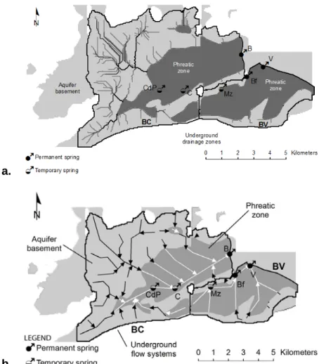
structuration of the geological model and on the availability of hydrological data, the three scenarios may be applied for delineating the phreatic zones. ________________________________________________ 136 Figure 5—8. Example of a KARSYS 3D aquifer model (Malard et al. [2015a]) for low-flow conditions; permanent springs are displayed in red (Beuchire, Bonnefontaine and Voyeboeuf) while temporary springs are labelled in orange (CdP, Creugenat and Mavaloz). The hydraulic gradient is mentioned (in %). As low-flow gradient exceeds 1‰, hydraulic discontinuities are expected between the observation points (i.e. springs, boreholes or sumps in caves). A small perched groundwater body (“X”) is supposed to develop in the northern part as a geological depression in the basement has been modeled. ___________________ 137 Figure 5—9. Principles of flows delineation in the vadose zone using GIS functionalities (ESRI, Spatial Analyst or ArcHydro Tools); a.) the main vadose drainage axes (black lines) are automatically computed on

the relief of the aquifer basement; b.) main axes are redrawn by hand. Here, vadose flows stop when

reaching the phreatic zone. White arrows refer to the expected flow directions in the phreatic zone. The main permanent springs draining the aquifers are B, Bf and V (see Malard et al. [2015a]). Delineation of the upstream heads of the flow lines makes it possible to delineate limits of the underground flow-system, i.e. the projected parts (plan view) of the aquifer that feeds the flow-system. ______________________ 138 Figure 5—10. Example of a KARSYS 3D conceptual model of the karst-flow system (example of the Beuchire-Creugenat karst system adapted from Vouillamoz et al. [2013]) __________________________ 139 Figure 5—11. Generic outputs of KARSYS; left: final KARSYS model of a karst aquifer in the Swiss Jura, right: associated documentation provided by the application of KARSYS (2D hydrogeological map, hydrogeological sheet describing system and catchment properties, and portable 3D model, usualy as .pdf3D) _______________________________________________________________________________ 140

Figure 5—12. Optimal karst-contexts for the application of the KARSYS approach (Ford and Williams [2007], modified). Optimal contexts entail: Alpine karst (Turk et al. [2014], Ballesteros et al. [2015b]; ), high karst plateau (Turk et al. [2013] ), lowland karst plateau (Malard et al. [2015a]) ________________ 142 Figure 5—13. Expected resolution of KARSYS models according to the size of the model [km2_{] and to the}

resolution of the input data. The resolution of geological data coming from boreholes or from hydrological data (i.e. springs) is about 1 m, whatever the size of the model. On the contrary, users are supposed to use geological maps of lower precision as the size of the model increases. This reduces the resolution of the resulting KARSYS model. Depending on the size of the model and on the resolution of the input data, users can expect a minimal resolution (the upper red curve) if they do not consider additional data of higher resolution. Considering a model of 100 km2_{, users may expect a minimal resolution of 50 m. __________ 145}

Figure 5—14. Architecture and content of the GIS database which has been developed for KARSYS; the

relation tables make it possible to link the objects inside a class (DATA) or between the two existing classes (“DATA” and “RESULTS”) _________________________________________________________________ 145 Figure 5—15. Principles of the validation process; resulting Model (n) is compared with validation Data (n+1), with independent data, principles or methods, and finally with the resulting Model (n+1). _______ 146 Figure 5—16. Hydrological information observed on a site and combined with the KARSYS principles may control the reliability of the interpreted geological structure on a site. A. No permanent springs do exist in

the central valley; a syncline structure with an underground threshold may explain the situation. B. A

permanent spring does emerge along the flank of the valley and a sinkhole lies on the other flank; a geological discontinuities (here a thrust) may explain the compartmentalization of the phreatic zones. __ 148 Figure 6—1. Examples of extensions to KARSYS; speleogenetic and inception-horizons models are

presented in Filipponi et al. [2012]; they are not further discussed here. ___________________________ 151 Figure 6—2. Superimposed head measurements of Beuchire (B), Creugenat (C), Champs-Montant (PdCM) and the POR3 borehole over June 2012 clearly evidence a hydraulic connection between these stations. The elevation for Creugenat and Beuchire is well measured while the precision of the altimetric leveling for PdCm and for POR3 is about 1 m. __________________________________________________________ 174 Figure 6—3. 1) As long as the Beuchire spring discharge rate remains lower than 700 L/s, the water level at

Creugenat does not react (~438 m a.s.l): both emergences are disconnected by a threshold (a) situated at this elevation. 2) As the Beuchire discharge rate exceeds 700 L/s the hydraulic head in Creugenat

progressively rises up until reaching a threshold (b) at 443 m a.s.l. This threshold may correspond to a by-pass conduit diverting the flow to the Beuchire spring, 3) as the discharge rate of the Beuchire spring

increases from 1’500 L/s to 2’000 L/s the water level in Creugenat does not change (~443 m). 4) As the

discharge rate exceeds 2’000 L/s the water level in Creugenat rises up again until reaching the outlet elevation (c) at 451 m a.s.l. _______________________________________________________________ 175 Figure 6—4. Hydraulic relationship between groundwater heads in POR3 and in Creugenat (for 3 selected flood events in 2002 and 2004); for a strong overflow event of Creugenat the water table in POR3 reaches a maximum at 447.5 m. The plateau at 443 m is clearly visible during the recession. _________________ 175 Figure 6—5. Inferred evolution of hydraulic heads of the BC conduits-system for high-flow conditions (phases a., b., and c.) induces the addition of a first threshold at 438 m a.s.l. and the addition of a perched

conduit at 443 m a.s.l. in order to explain that the discharge rate at the Beuchire spring increases while the hydraulic head in Creugenat does not rise anymore. Oscillations of the water table in POR3 act as an indicator of the hydraulic head evolution in the intermediate part of the conduit network. ____________ 177

Figure 6—6. Observations from June to July 2012 (i.e. for three flood events of moderate intensity); the water level in the POR3 borehole started to rise simultaneously to the Creugenat flooding while the water table in PdCM does not start rising before the Creugenat overflows. ______________________________ 177 Figure 6—7. Right: overflow of CdP during the flood event of April 4th_{, 1992. The supposed discharge rate}

on the picture is about 3 m3/s, even more (Maurice [1993]). Left: overflow of CdP during the flood event of August 2007 (9th_{); order of magnitude of the estimated peak discharge rate was about 2 to 4 m}3_{/s (picture}

from J-.C Bouvier)_______________________________________________________________________ 178 Figure 6—8. Supposed hydraulic relationships between the Creugenat discharge rate and the CdP discharge rate according to a min. and to a max. hypothesis. ___________________________________ 178 Figure 6—9. Flow-duration curves of Voyeboeuf and Bonnefontaine springs (2001-2013) _____________ 179 Figure 6—10. Hydraulic relationships between measured discharge rates at V and Bf springs for various periods in 2002 and 2004. ________________________________________________________________ 180 Figure 6—11. Overflow of Mz during the flood event of April 4th_{, 1992; the supposed discharge rate on the}

picture is in the order of a few hundreds of liters per second (Maurice [1993]). The discharge rate is small compared to the Creux-des-Près for the same event (see Figure 6—7). ____________________________ 180 Figure 6—12. Mz cave acts as an estavelle. When the cave becomes emissive, the ephemeral stream and the overflowed water are routed toward the BC karst system (B = Beuchire, C = Creugenat) ___________ 181 Figure 6—13. Three passes are evidenced through the aquiclude along the joint border of the BV and BC karst systems; at 450, 470 (“Le Banné” anticline) and at 480 m a.s.l. These passes may cause flow exchanges between these two systems depending on the fluctuations of the hydraulic gradient in the aquifer. According to this observation, the addition of three new hypothetic conduits could be suggested to the conduit network model (figure on the right, see §. 6.1) ______________________________________ 181 Figure 6—14. The shape of the hydraulic gradient for usual high-flow conditions can be sketched for BC and BV systems. CdP and Mz are still inactive for these conditions. _______________________________ 183 Figure 6—15. Routing principles of the RS semi-distributed software: details of a sub-catchment (i.e. for a given elevation range, here 200 m). Measured or inferred meteorological parameters (P, PET) are transferred to the GR3’ reservoir which provides a part of surface runoff (SWMM module) and a part of infiltration ____________________________________________________________________________ 186 Figure 6—16. Details of the snowpack sub-model of RS3.0. This simulates the evolution of the snow (deposit and melt) as a function of the temperature (T) and precipitation (P) producing an equivalent precipitation (Peq) used as input for the glacier or for the GR3 infiltration sub-model (fig. from e-dric

[2012]) _______________________________________________________________________________ 187 Figure 6—17. Details of the GR3 infiltration sub-model (e-dric [2012]); the GR3 is composed of two cascading reservoirs with distinct transfer functions depending on the water level. __________________ 188 Figure 6—18. Reservoirs organization in KRM_1; the model entails three cascading reservoirs: the Interception reservoir and the Upper and Lower reservoirs reflecting the tandem soil / epikarst. Peq is

computed with RS3.0. Resulting time series are the effective infiltration (i.e. the water penetrating the conduits). _____________________________________________________________________________ 191 Figure 6—19. Evolution of the seasonal storage capacity for the cultivated lands reservoir (left) and the forest canopy reservoir (right, Gerrits et al. [2010]) ____________________________________________ 192

Figure 6—20. Operating principle of the exchanger module; depending on a pseudo hydraulic head which is computed proportionally to the input flow-rates, it is assumed that a part of the effective infiltrations is stored in low permeability volumes surrounding the conduits. ___________________________________ 193 Figure 6—21. Principles of the exchanger functioning for a theoretical flood event; iin refers to the part of

water which is stored in the low permeability volumes while iout refers to the water released by the low

permeability volumes toward the conduits. __________________________________________________ 194 Figure 6—22. Workflow of recharge assessment over distributed surfaces; 1) subdivision of the B catchment into sub-catchments b1, b2, b3, etc.; 2) calculation of the soils properties over each

sub-catchment, 3) computation of distributed Peq and PET over each sub-catchment; 4) application of KRM_1

over each sub-catchment, starting from the respective soil occupation and input series Peq and PET; 5)

computation of the global recharge R over the catchment B and the distributed recharge over the sub-catchments Rb1, Rb2, Rb3, etc.; 6) further flow modelling (for instance hydraulic pipe-flow model). _____ 196

Figure 6—23. Land uses over the BC and BV catchment areas and location of the main meteorological stations FAH, MMO, THE, VAC and BRE. MTO is located 4 km eastward from VAC, out of the map. _____ 197 Figure 6—24. Calibration of KRM_1 for BC using ND Peq. The deviation with the observed value is

represented by the upper black curve (= simulation results – observed values at daily time-step) _______ 199 Figure 6—25. Five additional allogenic sub-catchments contribute to recharge the BV flow-system. The sum of the sub-catchments represents an additional contributing surface area of 3.3 km2_{. ____________ 200}

Figure 6—26. Calibration of the recharge model for BV using ND Peq (catchment enlarged to 22.2 km2). The

deviation with the observed value is represented by the upper black curve (= simulation results – observed values at daily time-step). ________________________________________________________________ 201 Figure 6—27. Simulated recharge for BC using the distributed Peq. The deviation is given by the upper black

curve (= simulation results – observed values at daily time-step). ________________________________ 203 Figure 6—28. Simulated recharge for BV using the distributed Peq. The deviation is given by the upper black

curve (=simulation results – observed values at daily time-step). _________________________________ 203 Figure 6—29. Simulated recharge for BC and BV for the flood event in August 2007. Over this period, measurements for comparison are only available for BV. As measurements for the Beuchire spring and for Creux-des-Près are missing, the simulated recharge for BC can only be compared to the measured discharge rate at Creugenat. ______________________________________________________________ 204 Figure 6—30. The BC/BV complete SWMM model; colors refer to the diameter of the conduits (Link Max. depth). The model entails the three additional thresholds between the two systems at 450, 470 and 480 m a.s.l., and the long and large by-pass conduit at 443 m in the downstream part of the BC karst system (3 m of diameter). __________________________________________________________________________ 209 Figure 6—31. Calibration results of the simulated regimes for the four outlets (B, C, V and Bf) over a selected period (Jan. to Jun. 2004) are compared with the measurements (daily mean values) and the results of the calibration performed with the simplified hydraulic model (see Appendix 10.14) _________ 210 Figure 6—32. Calibration results of the hydraulic heads variations for the borehole POR3 and the Mavaloz cave (Mz) over a selected period (Jan. to Jun. 2004) are compared with the measurements (only for POR3, daily mean values) and the results of the calibration performed with the simplified hydraulic model (see Appendix 10.14) ________________________________________________________________________ 212

Figure 6—33. Hydraulic model calibration; comparison of the Beuchire discharge rates with the simulated hydraulic heads in the Creugenat (see Figure 6—3 for comparison) _______________________________ 212 Figure 6—34. Simulated regime of the Beuchire permanent spring (left) and of the Creugenat overflow spring (right) for the flood-event of August 2007 [no measurements do exist at the Beuchire spring for comparison]; simulation results obtained with the simplified hydraulic model (see Appendix 10.14) are plotted for comparison. __________________________________________________________________ 213 Figure 6—35. Simulated regime of the Creux-des-Prés (CdP) overflow spring for the flood-event of August 2007 [no existing measurements]; simulation results obtained with the simplified hydraulic model (see Appendix 10.14) are plotted for comparison. _________________________________________________ 214 Figure 6—36. Simulated variations of the water table in POR3 for the flood-event of August 2007 [no existing measurements]; simulation results obtained with the simplified hydraulic model (see Appendix 10.14) are plotted for comparison. _________________________________________________________ 214 Figure 6—37. Computed regime of the Voyeboeuf and of the Bonnefontaine permanent springs for the flood-event of August 2007 [measured values for comparison]; simulation results obtained with the simplified hydraulic model (see Appendix 10.14) are plotted for comparison. _______________________ 215 Figure 6—38. Simulated overflow rates of the Mz cave during the flood event of August 2007 [no existing measurements for comparison]; simulation results obtained with the simplified hydraulic model (see Appendix 10.14) are plotted for comparison. _________________________________________________ 215 Figure 6—39. Schematic organization of the BC and BV karst conduit network as inferred from the KARSYS approach and from the hydraulic model ____________________________________________________ 217 Figure 6—40. Workflow of KARSYS extensions to assess the hydraulic functioning of karst flow-systems on the basis of a KARSYS model. 1) The 3D KARSYS model (output §. 5.2.1.4 for low-flow conditions) is further

analyzed for the generation of the conduit network (low-flow conditions) and the delineation of the catchment area (§. 6.1). 2) The catchment area and the discretized sub-catchments are implemented in

the recharge simulation model (here KRM_1, §. 6.3.3.1.1.2). 3) the generated geometry of the conduit

network is tested for high-flow conditions and adapted if necessary. 4) The adapted geometry of the

conduit network is used for the pipe-flow simulation model which considers the previously computed recharge 5) as input (§. 6.3.4). ____________________________________________________________ 219

Figure 6—41. Recommended workflow for assessing groundwater recharge depending on the dominating recharge process (“A” = elevation-dominated recharge, “B” = surface-processes-dominated recharge).

Distributed recharge may be further introduced as input for hydraulic models (such as SWMM©). _____ 221 Figure 6—42. Recommended recharge simulation models for karst aquifers in Switzerland. For grey zones, there is no recommended model, RS3.0 or KRM_1 may be a priori used providing the same interval of confidence; on the blue zones, KRM_1 could be applied with a high degree of confidence (dark blue) or a moderate degree of reliability (light blue); on the orange zones, RS3.0 should be applied with a high degree of confidence (dark orange) or a moderate degree of reliability (light orange).______________________ 222 Figure 6—43. Hydroclimatic contexts and type of the flow-system guide the selection of the appropriate recharge simulation model and the consideration of hydraulic processes via an additional model (here SWMM) or not in order to simulate the spring’s hydrograph ____________________________________ 223 Figure 6—44. Hydraulic functioning for high-flow conditions for three types of situations: a. Simple

the relationship between hydraulic head (H) and discharge rate (Q). Such relations provide indications on the conduit organization and on the existence of several conduit levels. ___________________________ 224 Figure 7—1. Karst regions of Switzerland and their expected hydroclimatic regime in 2085; regions with glacial, glacio-nival, nivo-glacial or nival regimes will become more pluvial; most of the Jura Mountains will move from a pluvial to a “pluvial of transition” regime, which is characterized by less recharge in winter/spring and an aggravated water deficit in summer. _____________________________________ 242 Figure 8—1. Synthesis of the KARSYS workflow including newly-developed extensions for a large range of applications ___________________________________________________________________________ 252 Figure 10—1. State of the documentation of karst aquifers in Switzerland at the end of the Swisskarst project _______________________________________________________________________________ 283 Figure 10—2. Relationship between karst groundwater temperature and the elevation of the spring (~160 karst springs); the correlation is significant although for similar elevation the difference in temperature may reach 3°C. Thermal springs could be identified from this relation. Systems for which the catchment area is well known are labeled separately giving an indication of the elevation-classes of the catchment area feeding the spring (<500 m, >500 m, >1000 m, >1500 m). Horizontal deviations in the temperatures distribution do not significantly depend on the elevation of the catchment. For instance, systems where elevation-classes exceed 1500 m are not closer to the min. than to the max. boundaries. _____________ 300 Figure 10—3. Seasonal variations of the groundwater temperature (monthly average) for selected karst flow-systems; a. the alpine Schlichenden Brünnen spring (Hölloch karst system, SZ), b. the elevated Jurassian Areuse Spring (NE), c. the low-elevated Jurassian Milandrine underground river (JU). The mean temperature fluctuates over the year of few degrees tenth (± 0.5°C for Schlichenden Brunnen and for Milandrine, ±1°C for Areuse, ± 0.8°C for Brunnmühle and up to 2.5°C for Malagne). The Orbe spring is a singular case as the seasonal amplitude of the temperature may reach 6 to 8°C… ___________________ 301 Figure 10—4. Whisker-Box plots showing the evolution of groundwater compounds in Jurassian karst aquifers for the first dataset (Jeannin et al. [Submitted]); the upper graphics refer to parameters related to carbonate dissolution while the lower graphics refer to other parameters showing a meaningful trend. For each parameter, plain values refer to the numbers of stations where the trend was identified (over a total of 40 stations), italic value gives the estimated rate of change (/year).Trends are further detailled hereafter. _____________________________________________________________________________ 306 Figure 10—5. Limitations of the KARSYS approach are of two types; limitations that are specific to the approach (approach-dependent) and limitations which are inherent to a man-made work and based on quantitative and qualitative data (approach-independent limitations). ____________________________ 325 Figure 10—6. The delineation of the flow-systems boundaries in the phreatic zone is difficult to assess in

case where the phreatic zone is drained by two or more permanent springs. Such boundaries are controlled by the hydraulic and they are expected to move depending on flow conditions. However, depending on the elevation of springs A. and B. and on the supposed hydraulic gradient in the phreatic zone, it is possible to approximate the location of the boundaries between the two flow-systems even if no further indications are provided. 1. If A. and B. are at the same elevation, we suppose the phreatic boundary to develop at

equal distance from the two springs; 2. If elevation A. > elevation B. and if ΔH/L is much lower than the

assumed gradient, the phreatic boundary will move upstream, close to the supposed conduit toward A. 3.

If elevation A. > elevation B. and if ΔH/L is close (or even bigger) than the assumed gradient, the phreatic boundary will move upstream of the phreatic conduit A. In this case, A. and B. are supposed to form an unique flow system as part of the upstream flow may reach B. __________________________________ 331

Figure 10—7. Schematic overview of the recharge model and the comparator in RS3.0 for BC and BV. Computed recharge at BV is compared to the summed discharge rate of Bf + V while the computed recharge at BC is compared to the summed discharge rate of B + C _______________________________ 355 Figure 10—8. Calibration of the RS3.0 recharge model over the period 2002-2004 for BC and BV compared to the cumulated discharge rates of their respective springs: Beuchire + Creugenat for BC and Bonnefontaine + Voyeboeuf for BV _________________________________________________________ 356 Figure 10—9. Results of recharge simulations for the flood event of August 2007 using RS3.0. Simulations could only be compared with measurements at BV as the Beuchire spring (BC) was not measured over this period. _______________________________________________________________________________ 358 Figure 10—10. Cross-correlation plots between the BC system’s regime and the measured precipitations at meteorological stations FAH, MMO, VAC, BRE, THE, MTO (daily time step) _________________________ 359 Figure 10—11. Normalized daily dispersion of gauged precipitation rates for the three meteorological stations FAH, BRE and THE; over the period, the global uncertainty in precipitation measurements is about 1% but for specific events, especially for higher rates of precipitation, dispersion may reach up to 30%... 360 Figure 10—12. Overview of the simplified SWMM hydraulic model of the BC/BV karst systems; colors refer to the diameter of the conduits. “Thr450” and “Thr470” refer to the supposed bypass conduits between BC and BV. _______________________________________________________________________________ 361 Figure 10—13. Calibration results for the discharge rates at Beuchire (B), Creugenat (C), Voyeboeuf (V) and Bonnefontaine (Bf) springs and for hydraulic heads at POR3 (borehole) and Mz (cave). _______________ 364 Figure 10—14. Hydraulic relationship between the discharge rate at the Beuchire spring and the evolution of the hydraulic head in the Creugenat (left: simulated, right: observed) ___________________________ 365 Figure 10—15. Simulation results of the simplified hydraulic model for the flood event of August 2007. Over this period, no measurements do exist for B, POR3, CdP and Mz. ____________________________ 367

–TABLES

Table 2—1. Values of effective porosity at the scale of a karst aquifer (review from literature) __________ 36 Table 2—2. Description of the karst hydrographic zones which form the karst flow-system (from Ford and Williams [2007], p 107); * refers to zones that may be traversed by conduits (permanently flooded in zone 3). It should be kept in mind that lower horizons of soils and epikarst zones may also be partially saturated.40 Table 2—3. Hydraulic gradient values measured in the phreatic zone for low-flow conditions in various karst flow-systems (literature review) _______________________________________________________ 44 Table 2—4. Measured values of high-flow hydraulic gradients in the phreatic zone for various karst

aquifers (literature review); most of them have been obtained by linear extrapolation between two observation points. ______________________________________________________________________ 47 Table 2—5. Various formulas to assess PET depending on the context, the available parameters and the computation time-step (literature review); ρA = air density [kg.m–3], ra = (s.m–1) aerodynamic resistance,

rc (s m–1) canopy surface resistance, es (kPa) saturated vapor pressure, ea (kPa) real vapor pressure, I =

monthly thermic index, fH Haude factor (in mmPa-1d-1), pD,S saturated vapor pressure (Pa), PD current vapor

pressure (Pa) and t the number of days for which the formulae applies. ____________________________ 51

Table 2—6. Values from the literature regarding the storage capacity for different compartments in karst aquifers (non-exhaustive); there are very few values for the epikarst and for the unsaturated zone. _____ 59

Table 2—7. Main concepts and key values for the development of hydrogeological characterization approaches _____________________________________________________________________________ 61 Table 3—1. Main karst-related problems when digging a tunnel (from Jeannin [2007]) ________________ 83 Table 3—2. Synthesis (non-exhaustive) of the problematic encountered in Swiss tunnels passing through a karst massif (sources: Schneider [1980]; Bianchetti [1993]; Jeannin and Wenger [1993]; Wildberger [1994], Bollinger and Kellerhals [2007]; Jeannin [2007]; Filipponi et al. [2012] and Anagnostou and Ehrbar [2013]) ________________________________________________________________________________ 84 Table 3—3. Overview of users and their interests for karst related information in Switzerland __________ 90 Table 3—4. Synthetic overview of users and their respective field of interest for karst-related information (focus on Switzerland). ___________________________________________________________________ 91 Table 4—1. Description of the main investigation methods on site _______________________________ 103 Table 4—2. Two kinds of tools may be distinguished; field tools and ex-situ tools____________________ 103 Table 4—3. Characteristics of karst hydrogeological maps obtained by the application of KARSYS; characterization scale and issues should be defined prior to apply KARSYS in order to provide the most appropriate type of map _________________________________________________________________ 107 Table 4—4. Advantages and disadvantages of the existing hydrological simulation approaches in karst _ 123 Table 4—5. Reliability of the usual simulation approaches in karst to address the three types of hydrological questions. Depending on their specificities and capabilities, the above-presented models may be well adapted, partially adapted, or unadapted to address the issues. _________________ 123 Table 5—1. Test sites where the KARSYS approach has been applied in the frame of the Swisskarst project126 Table 5—2. Main hydrological characteristics of karst springs as evidence for karst aquifers (adapted from Filipponi et al. [2012]) ___________________________________________________________________ 131 Table 5—3. Based on lithology, landforms, hydrological or physico-chemical evidences, the user assumes if the formation could be considered as karst aquifer, aquitard or if it is still undefined at that stage (ex: F2).132 Table 5—4. Depending on the availability of the hydrological data, three possible scenarios for the delineation of the phreatic zone do exist ____________________________________________________ 135 Table 5—5. Data-condition for the applicability of KARSYS Original 3D ____________________________ 144 Table 5—6. Validation means of the KARSYS geological 3D model ________________________________ 147 Table 5—7. Validation means of the KARSYS 3D aquifer model __________________________________ 149 Table 5—8. Validation means of the conceptual KARSYS 3D model _______________________________ 149 Table 6—1. Issues in flow simulation and criteria for choosing the most appropriate model ___________ 171 Table 6—2. Other minor springs emerging in the vicinity of the Beuchire spring and their respective min., mean and max. discharge rates. ___________________________________________________________ 172 Table 6—3. Available measurements; meteorological data come from Meteosuisse, hydrological ones come from MFR, RWB or the Jura canton (*coordinate Swiss Grid CH 1903). No measurements are available for Mavaloz and Creux-des-Prés. ___________________________________________________ 173 Table 6—4. Respective surface and land-uses of the BC and BV catchment areas ____________________ 197 Table 6—5. Monthly averages of evapotranspiration rates (in mm) computed at FAH over the period 2000-2012 (data MeteoSuisse). ________________________________________________________________ 198 Table 6—6. Optimized parameters for KRM_1 when applied to BC and BV flow-systems ______________ 199 Table 6—7. Contribution of KARSYS + hydrological and hydraulic extensions to recharge and flow modelling in karst aquifers compared to other recent models. ___________________________________ 220