Solid State Chemistry An Introduction Fourth Edition pdf - Web Education

(1)

K12133 Building a foundation with a thorough description of crystalline structures, Solid State Chemistry: An Introduction, Fourth Edition presents a wide range of the synthetic and physical techniques used to prepare and character-ize solids. Going beyond basic science, the book explains and analyzes modern techniques and areas of research. The book covers

• A range of synthetic and physical techniques used to prepare and characterize solids

• Bonding, superconductivity, and electrochemical, magnetic, optical, and conductive properties

• STEM, ionic conductivity, nanotubes and related structures such as graphene, metal organic frameworks, and FeAs superconductors • Biological systems in synthesis, solid state modeling, and

metamaterials

This largely nonmathematical introduction to solid state chemistry includes basic crystallography and structure determination, as well as practical examples of applications and modern developments to offer students the opportunity to apply their knowledge in real-life situations and serve them well throughout their degree course.

New in the Fourth Edition

• Coverage of multiferroics, graphene, and iron-based high temperature superconductors, the techniques available with synchrotron radiation, and metal organic frameworks (MOFs)

• More space devoted to electron microscopy and preparative methods • New discussion of conducting polymers in the expanded section on

carbon nanoscience

FOURTH EDITION

SOLID STATE CHEMISTRY

AN INTRODUCTION

ISBN: 978-1-4398-4790-9 9 0 0 0 0

A N I N T R O D U C T I O N

SO

LID

S

TA

TE

C

H

EM

IS

TR

Y

AN

IN

TR

O

DU

CT

IO

N

SMART MOORE FOURTH EDITION

(2)

(3)

(4)

(5)

CRC Press is an imprint of the

Taylor & Francis Group, an informa business Boca Raton London New York

(6)

CRC Press

Taylor & Francis Group

6000 Broken Sound Parkway NW, Suite 300 Boca Raton, FL 33487-2742

CRC Press is an imprint of Taylor & Francis Group, an Informa business No claim to original U.S. Government works

Version Date: 20120106

International Standard Book Number-13: 978-1-4398-4792-3 (eBook - PDF)

This book contains information obtained from authentic and highly regarded sources. Reasonable efforts have been made to publish reliable data and information, but the author and publisher cannot assume responsibility for the validity of all materials or the consequences of their use. The authors and publishers have attempted to trace the copyright holders of all material reproduced in this publication and apologize to copyright holders if permission to publish in this form has not been obtained. If any copyright material has not been acknowledged please write and let us know so we may rectify in any future reprint.

Except as permitted under U.S. Copyright Law, no part of this book may be reprinted, reproduced, transmit-ted, or utilized in any form by any electronic, mechanical, or other means, now known or hereafter inventransmit-ted, including photocopying, microfilming, and recording, or in any information storage or retrieval system, without written permission from the publishers.

For permission to photocopy or use material electronically from this work, please access www.copyright. com (http://www.copyright.com/) or contact the Copyright Clearance Center, Inc. (CCC), 222 Rosewood Drive, Danvers, MA 01923, 978-750-8400. CCC is a not-for-profit organization that provides licenses and registration for a variety of users. For organizations that have been granted a photocopy license by the CCC, a separate system of payment has been arranged.

Trademark Notice: Product or corporate names may be trademarks or registered trademarks, and are used

only for identification and explanation without intent to infringe.

Visit the Taylor & Francis Web site at http://www.taylorandfrancis.com and the CRC Press Web site at http://www.crcpress.com

(7)

Dedicated to our children

Sam and Laura, and

(8)

(9)

Preface to the Fourth Edition

Solid-state chemistry is still a rapidly advancing field, and the past few years have seen many new developments and discoveries in this field. This edition aims, as previously, not only to teach the basic science that underpins the subject, but also to direct the reader to the most modern techniques and to expanding and new areas of research. In order to do this, some of the subjects covered in the previous editions have either been briefly discussed or dropped altogether, to make way for the new. More space has been devoted to electron microscopy and to the techniques that are available with synchrotron radiation; there are new sections on nanomaterials and their synthesis and on computer modeling of solids, periodic mesoporous organo-silicas (PMOs), metal organic frameworks (MOFs), metal oxide frameworks, meta-materials, and multiferroics. The section on molecular metals has been dropped and the discussion on conducting polymers has been added at the end of the expanded section on carbon nanoscience. Throughout, new scientific terms and concepts are highlighted in bold typeface where they are first introduced.

We thank our colleagues and families, who have supported us throughout this project, Professor Mark Weller for his very helpful review, and, in particular, Drs. Craig McFarlane and Mike Mortimer and Professor Peter Atkins, who have generously given their time and expertise in explaining and correcting certain points of science.

We wish to acknowledge the use of the Chemical Database Service at Daresbury (Fletcher, D.A., Meeking, R.F., and Parkin, D., The United Kingdom Chemical Database Service, J. Chem. Inf. Comput. Sci. 36, 746–749, 1996), and the Inorganic Crystal Structure Database. (Berghoff, G and Brown, I.D., The Inorganic Crystal Structure Database (ICSD), in Crystallographic Databases, F. H. Allen et al., eds. Chester, International Union of Crystallography, 1987.) Also, WebLab Viewer Pro or Discovery Studio Visualiser from Accelerys Inc. was used to create the crystal structures.

Lesley Smart and Elaine Moore,

(18)

(19)

Preface to the Third Edition

Solid-state and materials chemistry is a rapidly moving field, and the aim of this edition has been to bring the text as up to date as possible with new developments. A few changes of emphasis have been made along the way. Single crystal X-ray dif-fraction has now been removed from Chapter 2 to make way for a wider range of the physical techniques used for characterising solids, and the number of synthetic techniques has been expanded in Chapter 3. Chapter 5 now contains a section on fuel cells and electrochromic materials. In Chapter 6, the section on low-dimensional sol-ids has been replaced with sections on conducting organic polymers, organic super-conductors and fullerenes. Chapter 7 now covers mesoporous solids and ALPOs, and Chapter 8 includes a section on photonics. Giant magnetoresistance (GMR) and colossal magnetoresistance (CMR) have been added to Chapter 9, and p-wave (trip-let) superconductors to Chapter 10. Chapter 11 is new, and it looks at the solid-state chemical aspects of nanoscience. We thank our readers for the positive feedback on the first two editions and for the helpful advice, which has led to this latest version. As ever, we thank our friends in the chemistry department at the OU, who have been such a pleasure to work with over the years and have made enterprises such as this possible.

(20)

(21)

Preface to the Second Edition

We were very pleased to be asked to prepare a second edition of this book. When we tried to decide on the changes (apart from updating) to be made, the advice from our editor was ‘if it ain’t broke, don’t fix it’. However, the results of a survey of our users requested about five new subjects but with the provisos that nothing was taken out, that the book did not get much longer and, above all, that it did not increase in price! So what you see here is an attempt to do the impossible, and we hope that we have satisfied some, if not all, of the requests.

The main changes from the first edition are two new chapters—Chapter 2 on X-ray diffraction and Chapter 3 on preparative methods. A short discussion of sym-metry elements has been included in Chapter 1. Other additions include an introduc-tion to ALPOs and to clay minerals in Chapter 7 and to ferroelectrics in Chapter 9. We decided that there simply was not enough room to cover the phase rule properly and for that we refer you to the excellent standard physical chemistry texts such as Atkins. We hope that the book now covers most of the basic undergraduate teaching material on solid-state chemistry.

We are indebted to Professor Tony Cheetham for kindling our interest in this subject with his lectures at Oxford University and the beautifully illustrated arti-cles that he and his collaborators have published over the years. Our thanks are also due to Dr. Paul Raithby for commenting on part of the manuscript.

As always, we thank our colleagues at the Open University for all their support and especially the members of the lunch club, who not only keep us sane but also keep us laughing. Finally, thanks go to our families for putting up with us and, in particular, to our children for coping admirably with two increasingly distracted academic mothers—our book is dedicated to them.

(22)

(23)

Preface to the First Edition

The idea for this book originated with our involvement in an Open University inor-ganic chemistry course (S343: Inorinor-ganic Chemistry). When the course team met to decide the contents of this course, we felt that solid-state chemistry had become an interesting and important area that must be included. It was also apparent that this area was playing a larger role in the undergraduate syllabus at many universities, due to the exciting new developments in the field.

Despite the growing importance of solid-state chemistry, however, we found that there were few textbooks that tackled solid-state theory from a chemist’s rather than a physicist’s viewpoint. Of those that did, most, if not all, were aimed at final-year undergraduates and postgraduates. We felt there was a need for a book written from a chemist’s viewpoint that was accessible to undergraduates earlier in their degree programme. This book is an attempt to provide such a text.

Because a book of this size could not cover all topics in solid-state chemistry, we have chosen to concentrate on structures and bonding in solids and on the interplay between crystal and electronic structure in determining their properties. Examples of solid-state devices are used throughout the book to show how the choice of a particular solid for a particular device is determined by the properties of that solid.

Chapter 1 is an introduction to crystal structures and the ionic model. It intro-duces many of the crystal structures that appear in later chapters and discusses the concepts of ionic radii and lattice energies. Ideas such as close-packed structures and tetrahedral and octahedral holes are covered here; these are used later to explain a number of solid-state properties.

Chapter 2 introduces the band theory of solids. The main approach is through the tight binding model, seen as an extension of the molecular orbital theory familiar to chemists. Physicists more often develop the band model through the free elec-tron theory, which is included here for completeness. This chapter also discusses electronic conductivity in solids and, in particular, properties and applications of semiconductors.

Chapter 3 is concerned with solids that are not perfect. The types of defects that occur and the way they are organised in solids form the main subject matter. Defects lead to interesting and exploitable properties and several examples of this appear in this chapter, including photography and solid-state batteries.

The remaining chapters each deal with a property or a special class of solids. Chapter 4 covers low-dimensional solids, the properties of which are not isotropic. Chapter 5 deals with zeolites, an interesting class of compounds used extensively in the industry (as catalysts, for example), the properties of which strongly reflect their structure. Chapter 6 deals with optical properties and Chapter 7 with magnetic properties of solids. Finally, Chapter 8 explores the exciting field of superconductors, in particular the relatively recently discovered high-temperature superconductors.

The approach adopted is deliberately nonmathematical and assumes only the chemical ideas that a first-year undergraduate would have. For example, differential

(24)

calculus is used on only one or two pages and nonfamiliarity with this would not hamper an understanding of the rest of the book; topics such as ligand field theory are not assumed.

As this book originated with an Open University text, it is only right that we should acknowledge the help and support of our colleagues on the course team, in particular Dr. David Johnson and Dr. Kiki Warr. We are also grateful to Dr. Joan Mason who read and commented on much of the script and to the anonymous reviewer to whom Chapman & Hall sent the original manuscript and who provided very thorough and useful comments.

The authors have been sustained through the inevitable drudgery of writing by an enthusiasm for this fascinating subject. We hope that some of this transmits itself to the student.

(25)

Authors

Lesley Smart studied chemistry at Southampton University, United Kingdom, and

after completing a PhD in Raman spectroscopy, she moved to a lectureship at the (then) Royal University of Malta. After returning to the United Kingdom, she took an SRC Fellowship to Bristol University to work on X-ray crystallography. From 1977 to 2009, she worked at the Open University chemistry department as a lecturer, senior lecturer and Molecular Science Programme director, and since retiring, holds an honorary senior lectureship there.

At the Open University, she was involved in the production of undergraduate courses in inorganic and physical chemistry and health sciences. She was the coor-dinating editor and an author of The Molecular World course, a series of eight books and DVDs copublished with the Royal Society of Chemistry, authoring two of these (2002), The Third Dimension and Separation, Purification and Identification. Her most recent books are (2007) Alcohol and Human Health and (2010) Concepts in

Transition Metal Chemistry. She has an entry in Mothers in Science: 64 Ways to

Have It All (downloadable from the Royal Society website). She has served on the Council of the Royal Society of Chemistry and as the chair of their Benevolent Fund.

Her research interests are in the characterisation of the solid state, and she has publications on single-crystal Raman studies, X-ray crystallography, Zintl phases, pigments and heterogeneous catalysis and fuel cells.

Elaine Moore studied chemistry as an undergraduate at Oxford University and then

stayed on to complete a DPhil in theoretical chemistry with Peter Atkins. After a two-year postdoctoral position at Southampton, she joined the Open University in 1975 as course assistant, becoming a lecturer in chemistry in 1977, senior lecturer in 1998 and reader in 2004. She has produced OU teaching texts in chemistry for courses at levels 1, 2 and 3 and written texts in astronomy at level 2 and physics at level 3. She is coauthor of Metal–Ligand Bonding, and the book Molecular Modelling and

Bonding, which forms part of the OU level 2 chemistry course, was copublished by the Royal Society of Chemistry as part of The Molecular World series. She oversaw the introduction of multimedia into chemistry courses and has designed multimedia material at levels 1, 2 and 3. She is coauthor of Metals and Life and of Concepts in

Transition Metal Chemistry, which are part of a level 3 Open University course in inorganic chemistry and copublished with the Royal Society of Chemistry.

Her research interests are in theoretical chemistry applied to solid-state systems and to NMR spectroscopy. She is author or coauthor of over 50 papers in scientific journals.

Solid-State Chemistry was first produced in 1992. Since then, it has been trans-lated into French, German, Spanish and Japanese and is currently being transtrans-lated into Arabic.

(26)

(27)

List of Units, Prefixes,

and Constants

BASIC SI UNITS

Physical Quantity (and Symbol) Name of SI Unit Symbol for Unit

Length (l) Metre m

Mass (m) Kilogram kg

Time (t) Second s

Electric current (I) Ampere A

Thermodynamic temperature (T) Kelvin K

Amount of substance (n) Mole mol

Luminous intensity (Iv) Candela cd

DERIVED SI UNITS

Physical Quantity (and Symbol) Name of SI Unit

Symbol for SI Derived Unit and Definition of Unit

Frequency (v) Hertz Hz (_=s−1₎

Energy (U), enthalpy (H) Joule J (= kg m2_s−2₎

Force Newton N (= kg m s−2 _{= J m}−1)

Power Watt W (= kg m2 _s−3_{= J s}−1₎

Pressure (p) Pascal Pa (= kg m−1_s−2_{= N m}−2_{= J m}−3₎

Electric charge (Q) Coulomb C (= A s)

Electric potential difference (V) Volt V (= kg m2_s−3_A−1_{= J A}−1_s−1₎

Capacitance (c) Farad F (= A2_s4_kg−1_m−2_{= A s V}−1_{= A}2_s2_J−1₎

Resistance (R) Ohm O (_{= V A}−1)

Conductance (G) Siemen S (= A V−1₎

Magnetic flux density (B) Tesla T (= V S m−2 _{= J C}−1 s m−2)

SI PREFIXES

10−18 10−15 10−12 10−9 10−6 10−3 10−2 10−1 103 ₁₀6 ₁₀9 ₁₀12 ₁₀15 ₁₀18

alto femto pico nano micro milli centi deci kilo mega giga tera peta exa

(28)

FUNDAMENTAL CONSTANTS

Constant Symbol Value

Speed of light in a vacuum c 2.997925 _{× 10}8_{m s}−1

Charge of a proton and charge of an electron

e 1.602189 × 10−19_C

Avogadro constant NA 6.022045 × 1023 mol−1

Boltzmann constant k 1.380662 × 10−23_{J K}−1_mol−1

Gas constant R = NAk 8.31441 × J K−1

Faraday constant F = NAe 9.648456 × 104 C mol−1

Planck constant h  = h 2π 6.626176 × 10−34_{J s} 1.05457 × 10−34_{J s} Vacuum permittivity ɛ0 8.854 × 10−12 F m−1 Vacuum permeability _μ0 4π×10−7 J s2 C−2 m−1 Bohr magneton μB 9.27402 × 10−24 J T−1 Electron g value ge 2.00232 Electron mass me 9.1095 × 10−31 kg Proton mass mp 1.6726 × 10−27 kg Neutron mass mn 1.6749 × 10−27 kg

MISCELLANEOUS PHYSICAL QUANTITIES

Name of Physical Quantity Symbol SI Unit

Enthalpy H J

Entropy S J K−1

Gibbs function G J

Standard change of molar enthalpy

�HmO J mol−1

Standard of molar entropy �SmO J K−1 mol−1

Standard change of molar Gibbs function

�GmO J mol−1

Wave number σ

λ

= 1 cm−1

Atomic number Z Dimensionless

Conductivity σ S m−1

Molar bond dissociation energy Dm J mol−1

Molar mass _M m n =⎛ ⎝⎜ ⎞ ⎠⎟ kg mol −1

(29)

THE GREEK ALPHABET alpha Α α nu Ν ν beta Β β xi Ξ ξ gamma _Γ _γ omicron _Ο _ο delta Δ δ pi Π π epsilon Ε ε rho Ρ ρ zeta _Ζ _ζ sigma _Σ _σ eta Η η tau Τ τ theta _Θ _θ upsilon _Υ _υ iota Ι ι phi Φ φ kappa Κ κ chi Χ χ lambda _Λ _λ psi _Ψ _ψ mu Μ µ omega Ω ω

(30)

PE R IO D IC C LA SS IF IC A TI O N OF T H E E LEM EN TS

(31)

1

An Introduction to

Crystal Structures

In the last few decades, research into solid-state chemistry has expanded very rapidly, fuelled at the start by the search for new and better materials and by the discovery in 1986 of ‘high-temperature’ ceramic oxide superconductors. We have seen immense strides in the development and understanding of nanotechnology, microporous and mesoporous solids, fuel cells and the giant magnetoresistance effect, to mention but a few areas. It would be impossible to cover all the develop-ments and topics in detail in an introductory text such as this, but we endeavour to give you a flavour of the excitement that some of the research has engendered and perhaps, more importantly, sufficient background with which to understand these developments and those that are yet to come.

Most substances, helium being a notable exception, if cooled sufficiently form a solid phase; the vast majority form one or more crystalline phases, where the atoms, molecules or ions pack together to form a regular repeating array. This book is con-cerned mostly with the structures of metals, ionic solids and extended covalent struc-tures; structures that do not contain discrete molecules as such, but that comprise extended arrays of atoms or ions. We look at the structure of, and bonding in, these solids, how the properties of a solid depend on its structure, and how the properties can be modified by changes to the structure.

1.1 INTRODUCTION

To understand the solid state, we need to have some insight into the structure of simple crystals and the forces that hold them together, so it is here that we start this book. Crystal structures are usually determined by the technique of X-ray

crystal-lography. This technique relies on the fact that the distances between the atoms in

the crystals are of the same order of magnitude as the wavelength of X-rays (of the order of 1 Å or 100 pm): a crystal thus acts as a three-dimensional diffraction grating to a beam of X-rays. The resulting diffraction pattern can be interpreted to give the internal positions of the atoms in the crystal very precisely, thus defining interatomic distances and angles. (Some of the principles underlying this technique are discussed in Chapter 2, where we review the physical methods available for characterising solids.) Most of the structures discussed in this book would have been determined in this way.

The structures of many inorganic crystal structures can be discussed in terms of the simple packing of spheres, so we will consider this first, before moving on to the more formal classification of crystals.

(32)

1.2 CLOSE PACKING

Think for a moment of an atom as a small hard sphere. Figure 1.1 shows two possible arrangements for a layer of such identical atoms. On squeezing the square layer in Figure 1.1a, the spheres would move to the positions in Figure 1.1b so that the layer takes up less space. The layer in Figure 1.1b—(layer A)—is said to be close-packed. The hollow spaces between the spheres are of two types, which have been marked with dots and crosses, respectively.

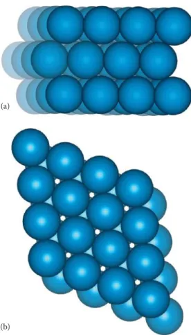
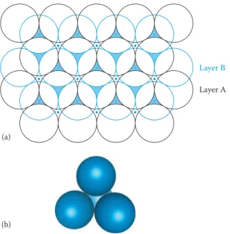
To build up a close-packed structure in three dimensions, we must now add a second layer—layer B. The spheres of the second layer can only sit in half of the hollows of the first layer, and layer B in Figure 1.2 (shown in blue) sits directly over the hollows marked with a cross (although it makes no difference which type we choose). When we come to add a third layer, there are again two possible options as to where it can go. First, it could go directly over layer A, in the unmarked hollows; if we repeated this stacking sequence, we would build up the layers ABABABA... and so on. This is known as hexagonal close packing (hcp) (Figure 1.3a). In this structure, the hollows marked with a dot are never occupied by spheres, leaving very small channels through the layers (Figure 1.3b).

(a)

(b)

(33)

Layer B

Layer A

FIGURE 1.2 Two layers of close-packed spheres.

(a)

(b)

FIGURE 1.3 (a) Three hcp layers showing the ABAB... stacking sequence. (b) Three hcp

(34)

In the second option, the third layer could be placed over those hollows, as in Figure 1.2b, marked with a dot. This third layer, which we now label C, would not be directly over either A or B, and the stacking sequence when repeated would be ABCABCABC... and so on. This is known as cubic close packing (ccp) (Figure 1.4). (The names hexagonal and cubic for these structures arise from the resulting sym-metry of the structures—this will be discussed more fully later on.)

Close packing represents the most efficient use of space when packing identical spheres—74% of the total volume is occupied by the spheres: the packing efficiency is said to be 74%. Each sphere in the structure is surrounded by twelve equidistant neighbours—six in the same layer, three in the layer above and three in the layer below: the coordination number of an atom in a close-packed structure is thus 12.

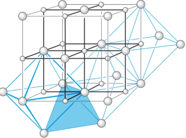
Another important feature of close-packed structures is the shape and number of the small amounts of space trapped in between the spheres. There are two differ-ent types of spaces within a close-packed structure: the first that we will consider is called an octahedral hole. Figure 1.5a shows two close-packed layers again, but with the octahedral holes shaded. Each of these holes is surrounded by six spheres, three in layer A and three in layer B; the centres of these spheres lie at the corners of an octahedron, hence the name (Figure 1.5b). If there are n spheres in the array, then there are also n octahedral holes.

Similarly, Figure 1.6a shows two close-packed layers, now with the second type of space, tetrahedral holes, shaded. Each of these holes is surrounded by four spheres with centres at the vertices of a tetrahedron (Figure 1.6b). If there are n spheres in the array, then there are 2n tetrahedral holes.

The octahedral holes in a close-packed structure are much bigger than the tet-rahedral holes—they are surrounded by six atoms rather than four. It is a matter of simple geometry to calculate that in a close-packed array of spheres of radius r, the radius of a sphere that will just fit in an octahedral hole is 0.414r. For a tetrahedral hole, the radius is 0.225r (Figure 1.7).

There are, of course, innumerable stacking sequences possible when repeating close-packed layers; however, hexagonal close-packed and cubic close-packed struc-tures are those of maximum simplicity and are those most commonly encountered in the crystal structures of the noble gases and of the metallic elements. Only two other stacking sequences are found in perfect crystals of the elements—an ABAC repeat in La, Pr, Nd and Am; and a nine-layer repeat ABACACBCB in Sm.

(35)

(a)

(b)

Layer A

Layer B

FIGURE 1.5 (a) Two layers of close-packed spheres with the enclosed octahedral holes

shaded. (b) A computer representation of an octahedral hole.

(a)

(b)

Layer A

Layer B

FIGURE 1.6 (a) Two layers of close-packed spheres with the tetrahedral holes shaded.

(36)

1.3 BODY-CENTRED AND PRIMITIVE STRUCTURES

Some metals do not adopt a close-packed structure, but have a slightly less efficient packing method: it is the body-centred cubic (bcc) structure, shown in Figure 1.8. (Unlike the previous diagrams, the positions of the atoms are now represented here, and in subsequent diagrams, by small spheres that do not touch each other: this is merely a device to open up the structure and allow it to be seen more clearly. The whole question of atom and ion size is discussed in Section 1.6.4.) In this structure, an atom in the middle of a cube is surrounded by eight identical and equidistant atoms at the corners of the cube, the coordination number has dropped from 12 to 8 and the packing efficiency is now 68%, compared with 74% for close packing.

The simplest of the cubic structures is the primitive cubic structure. This is built by placing square layers like the one shown in Figure 1.1a, directly on top of one

FIGURE 1.8 A body-centred cubic array.

(a)

(b)

FIGURE 1.7 (a) A sphere of radius 0.414r fitting into an octahedral hole. (b) A sphere of

(37)

another. Figure 1.9a illustrates this, and we can see in Figure 1.9b that each atom sits at the corner of a cube. The coordination number of an atom in this structure is six.

The majority of metals have one of the three basic structures: hcp, ccp or bcc; polonium alone adopts the primitive structure. The distribution of the packing types among the most stable forms of the metals at 298 K is shown in Figure 1.10. As we noted earlier, very few metals have a mixed hcp/ccp structure of a more

(a)

(b)

FIGURE 1.9 (a) Two layers of a primitive cubic array. (b) A cube of atoms from this array.

Li Be Sc Y Lu Ti Zr Hf V Nb Ta Cr Mo W Mn Tc Re Fe Ru Os Co Rh Ir Ni Pd Pt Cu Ag Au Zn Cd Hg Ga Al In Tl Sn Pb Na Mg Ca Sr Ba K Rb Cs La Ce ccp hcp bcc hcp/ccp Pr Nd Pm Sm Eu Gd Tb Dy Ho Er Tm Yb

(38)

complex type. The structures of the actinoids tend to be rather complex and are not included.

1.4 SYMMETRY

Before we take the discussion of crystalline structures any further, we will look at the symmetry displayed by chemical species. The concept of symmetry is an extremely useful one when it comes to describing the shapes of both individual molecules and regular repeating structures, as it provides a way of describing simi-lar features in different structures so that they become unifying features. The sym-metry of objects in everyday life is something that we tend to take for granted and recognise easily without having to think about it. Take some simple examples illustrated in Figure 1.11. If we imagine a mirror dividing a spoon in half along the plane indicated, then we can see that one half of the spoon is a mirror image or reflection of the other half. Similarly with the paintbrush, only now there are two

(a) (b)

(c) (d)

FIGURE 1.11 Common objects displaying symmetry: (a) a spoon, (b) a paintbrush, (c) a

(39)

mirror planes at right angles which divide it. This symmetry feature is called a

plane of symmetry.

Objects can also possess rotational symmetry. In Figure 1.11c, imagine an axle passing through the centre of the snowflake; in the same way as a wheel rotates about an axle, if the snowflake is rotated through one-sixth of a revolution, then the new position is indistinguishable from the old. Similarly, in Figure 1.11d, rotating the seven-sided UK 50p coin about a central axis by one-seventh of a revolution brings us to the same position as we started (ignoring the pattern on the surface). These axes are known as axes of symmetry or rotational axes. The symmetry axes and planes possessed by objects are examples of symmetry elements.

1.4.1 Symmetry NotatioN

Two forms of symmetry notation are in common use, and as chemists we will come across both. The Schoenflies notation is useful for describing the symmetry of individual molecules and is used by spectroscopists. The Hermann–Mauguin notation can be used to describe the symmetry of individual molecules; addition-ally, it is also used to describe the relationship between different molecules in space—their so-called space symmetry—and so it is the form most commonly met in crystallography and in the solid state, although both are used. Here, we give the Schoenflies notation in parentheses after the Hermann–Mauguin notation.

1.4.2 axeS of Symmetry

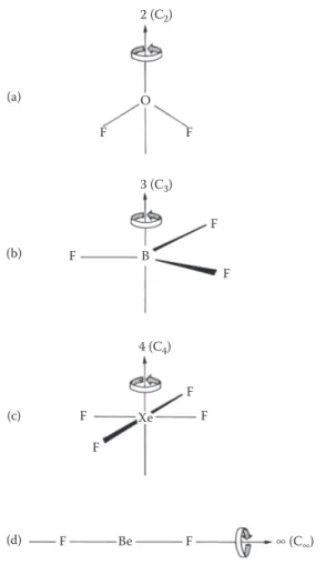
In the same way that we have previously seen for the snowflake and the 50p coin, molecules can also possess rotational symmetry. Figure 1.12 illustrates this for sev-eral molecules.

In Figure 1.12a, the rotational axis is shown as a vertical line through the O atom in OF2; rotation about this line by 180° in the direction of the arrow produces an

identical-looking molecule. The axis of symmetry in this case is a twofold axis because we have to perform the rotation twice to return the molecule to its starting position.

Axes of symmetry are denoted by the symbol n (Cn), where n is the order of the axis. So the rotational axis of the OF2 molecule is 2 (C2).

The BF3 molecule in Figure 1.12b possesses a threefold axis of symmetry (3 (C3))

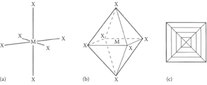
because each one-third of a revolution leaves the molecule looking the same, and three turns bring the molecule back to its starting position. In the same way, the XeF4

molecule in Figure 1.12c has a fourfold axis (4 (C4)) and four quarter turns are

nec-essary to bring it back to its starting position. Notice that this molecule also has C2

rotational axes at right angles to the C4 axis; this highest-order axis is then denoted

as the principal axis. All linear molecules have an ∞ (C_∞) axis, which is illustrated for the BeF2 molecule in Figure 1.12d; however small an angle of rotation it always

looks identical. The smallest angle of rotation possible is 1/∞, and so this principal axis is an infinite-order axis of symmetry.

(40)

1.4.3 PlaNeS of Symmetry

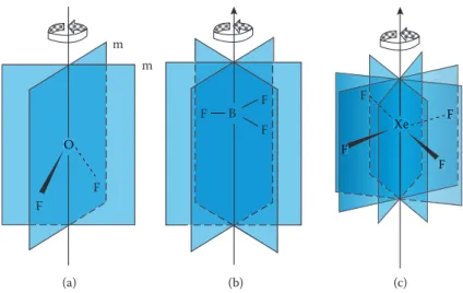
Mirror planes occur in isolated molecules and in crystals such that everything on one side of the plane is a mirror image of the other. In a structure such a mirror plane is given the symbol m (σ). Molecules may possess one or more planes of

symmetry, and the diagrams in Figure 1.13 illustrate some examples. The planar

OF2 molecule has two planes of symmetry (Figure 1.13a): one is the plane of the

molecule and the other is at right angles to the former. For all planar molecules, the plane of the molecule is a plane of symmetry. The diagrams for BF3 (and also

planar molecules) only show the planes of symmetry that are perpendicular to the plane of the molecule. A symmetry plane that is parallel to the principal axis is known as vertical (σv) and the one perpendicular to it is known as horizontal (σh). A

third type of symmetry plane that bisects the angle between 2 twofold rotation axes perpendicular to the principal axis, as shown in Figure 1.13c for XeF4, is known as dihedral (σd). (a) 2 (C2) 3 (C3) 4 (C4) Xe F F F F F Be F ∞ (C∞) F B F F O F F (b) (c) (d)

FIGURE 1.12 Axes of symmetry in molecules: (a) twofold axis in OF2, (b) threefold axis in

(41)

1.4.4 iNverSioN

In this section, we show the third symmetry element called inversion through an

inversion centre or centre of symmetry; it is given the symbol ₁(i). In this element, you have to imagine a line drawn from any atom in the molecule, through the centre of symmetry and then continued for the same distance the other side; if, for every atom, this meets with an identical atom on the other side, then the molecule has a centre of symmetry. Of the molecules in Figure 1.12, XeF4 and BeF2 both have a

cen-tre of symmetry, while BF3 and OF2 do not. The benzene molecule (C6H6) possesses

a centre of symmetry in the middle of the ring.

The next symmetry element is described differently in the Schoenflies and Hermann–Mauguin notations.

1.4.5 iNverSioN axeS aNd imProPer Symmetry

axeS aNd the ideNtity elemeNt

The two following symmetry elements, inversion axis and improper symmetry axis, give the same result, but are described differently in the two systems. Both descrip-tions use a combination of the symmetry elements described above. The Hermann– Mauguin inversion axis is a combination of rotation and inversion and is given the symbol n. The symmetry element consists of a rotation by 1/n of a revolution about the symmetry axis, followed by inversion through the centre of symmetry. An example of a ₄ inversion axis is shown in Figure 1.14 for a tetrahedral molecule such as CF4. The

molecule is shown inside a cube as this makes it easier to see the symmetry elements. Anticlockwise rotation about the axis through 90_{° takes F}1 to the position shown as

a dotted F, and inversion through the centre then takes this atom to the F3 position.

The equivalent symmetry element in the Schoenflies notation is the improper

axis of symmetry (S_n) or the rotation–reflection axis, which, as its name suggests,

F F F Xe (c) FF F F F X Xe X (b) F B F F (a) O O m m F F F

FIGURE 1.13 Planes of symmetry in molecules: (a) planes of symmetry in OF2, (b) planes

(42)

is a combination of rotation and reflection. The symmetry element consists of a rota-tion by 1/n of a revolurota-tion about the axis, followed by reflecrota-tion through a plane at right angles to the axis. Figure 1.14 thus also shows an S4 axis: F1 rotates to the dotted

position and then reflects to F2. The equivalent inversion axes and improper

symme-try axes for the two systems are shown in Table 1.1.

F3 F2 F4 F1 C 4 (S4)

FIGURE 1.14 The 4 (S4) inversion (improper) axis of symmetry in the tetrahedral CF4

molecule.

TABLE 1.1

Equivalent Symmetry Elements in the Schoenflies and Hermann–Mauguin Systems

Schoenflies Hermann–Mauguin S1≡ m 2≡ m S2≡ i 1 ≡ i S3 6 S4 4 S6 3

(43)

The group of five symmetry elements is completed by the so-called identity

element (E), which is no change—the equivalent of multiplying by 1.

1.4.6 oPeratioNS

Whereas the symmetry elements are essentially static properties of the object, actions such as rotating or reflecting a molecule are called symmetry operations, and the five symmetry elements have five symmetry operations associated with them. Their notation is distinguished from those of the elements by a caret; thus, _Ĉn is the rota-tion of a molecule around an axis and Ê is the identity operarota-tion.

The group of all the symmetry operations acting on a single object to describe the repetition of identical parts of the object while one point remains fixed is known as its point group. For the determination of the point groups of common molecules, we refer you to the standard texts on the subject (see the Further Reading at the end of the book).

1.4.7 Symmetry iN CryStalS

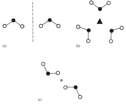
The discussion so far has only shown the symmetry elements that belong to indi-vidual molecules. However, in the solid state, we are interested in regular arrays of atoms, ions or molecules, and they too are related by these same symmetry ele-ments. Figure 1.15 shows examples (not real) of how molecules could be arranged in

(c)

(a) (b)

FIGURE 1.15 Symmetry in solids: (a) two OF2 molecules related by a plane of symmetry,

(b) three OF2 molecules related by a threefold axis of symmetry and (c) two OF2 molecules

(44)

a crystal. In Figure 1.15a, two OF2 molecules are related to one another by a plane

of symmetry; in Figure 1.15b, three OF2 molecules are related to one another by a

threefold axis of symmetry; and in Figure 1.15c, two OF2 molecules are related by a

centre of inversion. Notice that in Figure 1.15b and 1.15c, the molecules are related in space by a symmetry element that they themselves do not possess; this is said to be their site symmetry.

1.5 LATTICES AND UNIT CELLS

Crystals are regular-shaped solid particles with flat shiny faces. In 1664, Robert Hooke first noted that the regularity of their external appearance is a reflection of a high degree of internal order. Crystals of the same substance, however, vary in shape considerably. In 1671, Steno observed that this is not because their internal structure varies, but because some faces develop more than others. The angles between similar faces on different crystals of the same substance are always iden-tical. The constancy of the interfacial angles reflects the internal order within the crystals. Each crystal is derived from a basic ‘building block’ that repeats over and over again, in all directions, in a perfectly regular way. This building block is known as the unit cell.

In order to talk about and compare the many thousands of crystal structures that are known, there has to be a way of defining and categorising the structures. This is achieved by defining the shape, symmetry and also the size of each unit cell and the positions of the atoms within it.

1.5.1 lattiCeS

The simplest regular array is a line of evenly spaced objects such as that depicted by the commas in Figure 1.16a. There is a dot at the same place in each object: if we now remove the objects leaving the dots, we have a line of equally spaced dots of spacing a (Figure 1.16b). The line of dots is called the lattice, and by definition each lattice point (dot) has identical surroundings. This is the only example of a one-dimensional lattice and it can vary only in the spacing a. There are five possible two-dimensional lattices, and everyday examples of these can be seen all around in wallpapers and tiling.

(a)

a

a (b)

(c)

(45)

1.5.2 oNe- aNd two-dimeNSioNal UNit CellS

The unit cell for the one-dimensional lattice in Figure 1.16a lies between the two vertical lines. If we took this unit cell and repeated it over and over again, we would reproduce the original array. Notice that it does not matter where in the structure we place the lattice points as long as they each have identical surroundings. In Figure 1.16c, we have moved the lattice points and the unit cell, but repeating this unit cell will still give the same array—we have simply moved the origin of the unit cell. There is never one unique unit cell that is ‘correct’; there are always many that could be chosen and the choice depends both on convenience and convention. This is equally true in two and three dimensions.

The unit cells for the two-dimensional lattices are parallelograms with their cor-ners at equivalent positions in the array, that is, the corcor-ners of a unit cell are

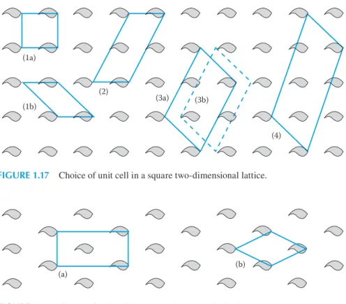
lat-tice points. In Figure 1.17, we show a square array with several different unit cells depicted. All of these, if repeated, would reproduce the array, but it is conventional to choose the smallest cell that fully represents the symmetry of the structure. Both unit cells (1a) and (1b) are of the same size, but clearly (1a) shows that the array is square, and this would be the conventional choice. Figure 1.18 demonstrates the same principles but for a centred rectangular array, where (a) would be the conven-tional choice because it includes information on the centring; the smaller unit cell (b)

(1a)

(1b)

(2)

(3a) _(3b)

(4)

FIGURE 1.17 Choice of unit cell in a square two-dimensional lattice.

(a) (b)

(46)

loses this information. It is always possible to define a noncentred oblique unit cell, but information about the symmetry of the lattice may be lost by doing so.

Unit cells such as (1a) and (1b) in Figure 1.17 and (b) in Figure 1.18 have a lattice point at each corner. However, they each contain a total of one lattice point because each lattice point is shared by four adjacent unit cells. They are known as primitive

unit cells and are given the symbol P. The unit cell marked (a) in Figure 1.18 contains

a total of two lattice points—one from the shared four corners and the other totally enclosed within the cell. This cell is said to be centred and is given the symbol C.

1.5.3 traNSlatioNal Symmetry elemeNtS

In Section 1.4, we introduced you to the idea of symmetry, both in individual mol-ecules and for extended arrays of molmol-ecules such as those found in crystals. Before going on to discuss three-dimensional lattices and unit cells, it is important to intro-duce two more symmetry elements; these elements involve translation and are only found in the solid state.

The glide plane combines translation with reflection. Figure 1.19 shows an example of this symmetry element. The diagram shows part of a repeating three-dimensional structure projected onto the plane of the page; the circle represents a molecule or ion in the structure and there is a distance a between identical posi-tions in the structure in the x direction (this follows the convention that a unit cell based on the x, y and z axes has unit cell dimensions a, b and c in those respective directions). The _{+ sign next to the circle indicates that the molecule lies above the} plane of the page in the z direction. The plane of symmetry is in the xz plane per-pendicular to the page and is indicated by the dashed line. The symmetry element consists of reflection through this plane of symmetry, followed by translation. The translation can be either in the x or in the z direction (or along a diagonal) and the translation distance is half of the repeat distance in that direction. In the example illustrated, the translation takes place in the x direction; the repeat distance between identical molecules is therefore a, and the translation is by a/2. This symmetry

Glide _Glide direction y x z plane a/2 a + + +

(47)

element is called an a glide. If the translation had been along the z direction, the translation would have been by c/2 and is called a c glide.

You will notice two things about the molecule generated by this symmetry ele-ment: first, it still has a _{+ sign against it, because the reflection in the plane leaves the}

z coordinate the same and, second, it now has a comma on it. Some molecules when

21 Screw axis c/2 + + y x z c −

FIGURE 1.20 A 21 screw axis along z.

2 21

32 31 3

(48)

reflected through a plane of symmetry are enantiomorphic, which means that they are not superimposable on their mirror image: the presence of the comma indicates that this molecule could be an enantiomorph.

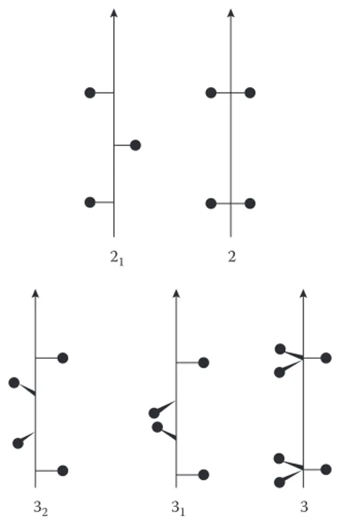
The screw axis combines translation with rotation. Screw axes have the general symbol ni, where n is the rotational order of the axis, that is, twofold, threefold, etc., and the translation distance is given by the ratio i/n. Figure 1.20 illustrates a 21 screw axis. In this example, the screw axis lies along the z direction and so the

translation must also be in the z direction by c/2, where c is the repeat distance in the z direction. Notice that in this case, the molecule starts above the plane of the page (indicated by the _{+ sign), but the effect of a twofold rotation is to take it below} the plane of the page (_{− sign). Figure 1.21 probably illustrates this more clearly and} also shows the different effects that the rotational and screw axes of the same order have on a repeating structure. Rotational and screw axes produce objects that are superimposable on the original. All other symmetry elements—glide plane, sym-metry plane, inversion centre and inversion axis—produce a mirror image of the original.

1.5.4 three-dimeNSioNal lattiCeS aNd their UNit CellS

There are seven lattice systems defined by their symmetry: triclinic, monoclinic, orthorhombic, tetragonal, rhombohedral, hexagonal and cubic (Table 1.2).

As we saw in two dimensions, a lattice can always be defined by a primitive unit cell (P) with a lattice point at each corner; the same is true in three dimensions. However, in three dimensions, there are three other types of lattices with unit cells

TABLE 1.2

Seven Lattice Systems

System Unit Cell Minimum Symmetry Requirements

Triclinic _{α ≠ β ≠ γ ≠ 90°} a ≠ b ≠ c None Monoclinic α = γ = 90° β ≠ 90° a ≠ b ≠ c

One twofold axis or one symmetry plane

Orthorhombic α = β = γ = 90° a ≠ b ≠ c

Any combination of three mutually perpendicular twofold axes or planes of symmetry

Tetragonal α = β = γ = 90°

a = b ≠ c

One fourfold axis or one fourfold improper axis Rhombohedral _{α = β = γ ≠ 90°}

a = b = c

One threefold axis

Hexagonal α = β = 90°

γ = 120° a = b ≠ c

One sixfold axis or one sixfold improper axis

Cubic α = β = γ = 90°

a = b = c

(49)

larger than the primitive ones; all four types are listed next and are illustrated in Figure 1.22.

1. The primitive unit cell—symbol P—has a lattice point at each corner. 2. The body-centred unit cell—symbol I—has a lattice point at each corner

and one at the centre of the cell.

3. The face-centred unit cell—symbol F—has a lattice point at each corner and one at the centre of each face.

(a) (b)

(c)

(d)

FIGURE 1.22 (a) Primitive (P), (b) body-centred (I), (c) face-centred (F) and (d) face-centred

(50)

4. The face-centred unit cell—symbol A, B or C—has a lattice point at each corner, and one at the centres of a pair of opposite faces, for example, an A-centred cell has lattice points at the centres of the bc faces.

These lattice types are distributed among the lattice systems to give the 14 Bravais lattices listed in Table 1.3. Notice, for instance, that it is not possible to have an A-centred (or B- or C-centred) cubic unit cell; if only two of the six faces are centred, the unit cell necessarily loses its cubic symmetry.

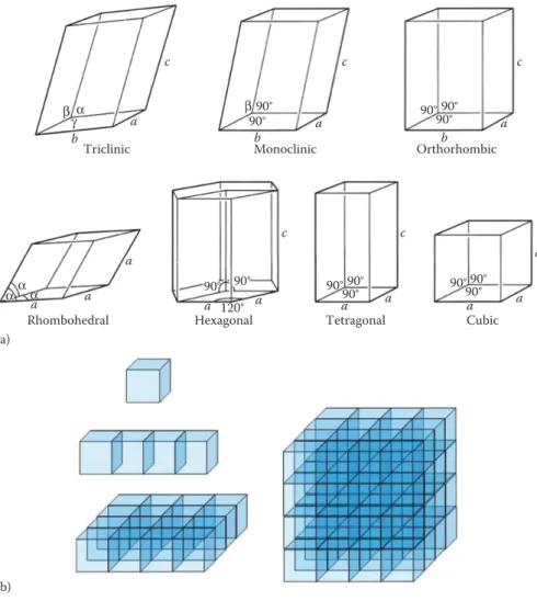
The unit cell of a three-dimensional lattice is a parallelepiped defined by three distances a, b and c, along the x, y and z axes, respectively, and three angles _α, β and γ, where α is the angle between the y and z axes; β between x and z; and γ between x and y (Figure 1.23). Because the unit cells are the basic building blocks of the crystals, they are space-filling, that is, they must pack together to fill all space. The unit cells of the seven lattice systems are illustrated in Figure 1.24. The seven lattice systems together with the shapes of their unit cells, as determined by mini-mum symmetry requirements, are detailed in Table 1.3.

TABLE 1.3

Bravais Lattices

Lattice System Lattice Types

Cubic P, I, F Tetragonal P, I Orthorhombic P, C, I, F Hexagonal P Rhombohedral Ra Monoclinic P, C Triclinic P

a _{The primitive unit cell of the rhombohedral}

system is normally given the symbol R.

x y z b β a c γ α

(51)

The symmetry of a crystal is a point group taken from a point at the centre of a perfect crystal and the set of symmetry operations leave this point fixed while mov-ing each atom of the crystal to the position of an atom of the same kind. Only certain point groups are possible because of the constraint made by the fact that unit cells must be able to stack exactly with no spaces—thus, for instance, only one-, two-, three-, four- and sixfold rotational axes are possible. Combining this with the planes of symmetry and centres of symmetry, we find that there are 32 crystallographic point groups compatible with the translational symmetry in three dimensions. If we combine the 32 crystal point groups with the 14 Bravais lattices, we find that there are 230 three-dimensional space groups that crystal structures can adopt, that is, 230 different space-filling patterns. These are all documented in the International Tables for Crystallography (see Bibliography at the end of the book).

Triclinic

Rhombohedral Hexagonal Tetragonal Cubic

Monoclinic Orthorhombic 90° 90° 90° 90° 90° 90° 90° 90° 120° 90° 90° 90° 90° 90° β β a a a a a a a a a a a a a b b b c c c c c γα α α α (a) (b)

FIGURE 1.24 (a) Unit cells of the seven crystal systems. (b) Assemblies of cubic unit cells

(52)

It is important not to lose sight of the fact that the lattice points represent

equiva-lent positions in a crystal structure and not atoms. In a real crystal, a lattice point could be occupied by an atom, a complex ion, a molecule or even a group of mol-ecules. The lattice points are used to simplify the repeating patterns within a struc-ture, but they tell us nothing of the chemistry or bonding within the crystal—for that we have to include the atomic positions; this we will do later in the chapter when we look at some real structures.

It is instructive to note how much of a structure these various types of unit cell represent. We noted a difference between the centred and the primitive two-dimensional unit cells, where the centred cell contains two lattice points whereas the primitive cell contains only one. We can work out similar occupancies for the three-dimensional case. The number of unit cells sharing a particular lattice point depends on its site. A corner site is shared by eight unit cells, an edge site by four, a face site by two and a lattice point at the body centre is not shared by any other unit cell (Figure 1.25). Using these figures, we can work out the number of lattice points in each of the four types of cells in Figure 1.22. The results are listed in Table 1.4.

(a)

(b)

(c)

FIGURE 1.25 Unit cells showing a molecule on (a) a face, (b) an edge and (c) a corner.

TABLE 1.4

Number of Lattice Points in the Four Types of Unit Cell

Name Symbol

Number of Lattice Points in Unit Cell

Primitive P 1

Body-centred I 2

Face-centred A or B or C 2

(53)

1.5.5 miller iNdiCeS

The crystal faces, both when they grow and when they are formed by cleavage, tend to be parallel either to the sides of the unit cell or to the planes in the crystals that contain a high density of atoms. It is useful to be able to refer to both the crystal faces and the planes in the crystals in some way—to give them a label—and this is usually done by using Miller indices.

First, we will describe how Miller indices are derived for lines in two-dimensional nets and then move on to look at planes in three-dimensional lattices. Figure 1.26 shows a rectangular net with several sets of lines, and a unit cell is marked on each set with the origin of each in the bottom left-hand corner corresponding to the direc-tions of the x and y axes. A set of parallel lines are defined by two indices, h and

k, where h and k are the number of parts into which a and b, the unit cell edges, are divided by the lines. Thus, the indices of a line hk are defined so that the line intercepts a at a/h and b at b/k. Start by finding a line next to the one passing through the origin. In the set of lines marked A, the line next to the one passing through the origin leaves a undivided (a/1), but divides b into two (b/2); both intercepts lie on the positive side of the origin, so in this case the indices of the set of lines hk are 12, called the ‘one-two’ set. If the set of lines lies parallel to one of the axes, then there is no intercept and the index becomes zero. If the intercepted cell edge lies on the nega-tive side of the origin, then the index is written with a bar on the top, for example, ₂, called ‘bar-two’. Notice that if we had selected the line on the other side of the origin in A, we would have indexed the lines as the _{1 2}; there is no difference between the two pairs of indices and always the hk and the _{h k} lines are the same set of lines. Try Question 5 for more examples. Notice also, in Figure 1.26, that the lines with the lower indices are more widely spaced.

a b y A E D C B x

(54)

The Miller indices for planes in three-dimensional lattices are given by hkl, where

l is now the index for the z axis. The principles are exactly the same. Thus, a plane is indexed hkl when it makes intercepts a/h, b/k and c/l with the unit cell edges a, b and

c, respectively. Figure 1.27 shows some cubic lattices with various planes shaded. The positive directions of the axes are marked and these are orientated to conform with the conventional right-hand rule, as illustrated in Figure 1.28. In Figure 1.27a, the shaded planes lie parallel to y and z, but leave the unit cell edge a undivided;

(a) x y z (b) (c) (d) a

FIGURE 1.27 (a–c) Planes in a face-centred cubic lattice. (d) Planes in a body-centred cubic