Kin-dependent dispersal influences relatedness and genetic structuring in a lek system

(1)

APPENDIX A: study area, capture-recapture survey, and DNA

analyses

1. Study site, sampling design and sample collection

The Vosges Mountains are dominated by a south–north oriented ridge and small valleys separating low-altitude mountains. Until the 1970s, capercaillie distribution range extended to low low-altitude forests (400– 500 m a.s.l.) dominated by Silver fir (Abies alba), Beech (Fagus sylvatica) and Scot pine (Pinus

sylvestris), with a dense Bilberry (Vaccinium myrtillus) cover. Capercaillie distribution range contracted

and the species nowadays persists at higher altitude (800–1250 m a.s.l.), in disconnected patches of mixed forest dominated by Silver fir, with Beech, Maple (Acer sp.) and Norway spruce (Picea abies). Capercaillie is also found at the subalpine range in Beech dominated forests and above tree line in moorlands dominated by ericaceous shrubs, where females find suitable habitat for the rearing of their broods. Lekking arenas are generally localised at the edges of moorlands dominated by ericaceous shrubs or moors. Scot pine needles is the preferred food source during winter, substituted by Silver fir needle in areas where Scot pine is absent (Lefranc & Preiss 2008).

As part of the routine monitoring of capercaillie, volunteers of the Groupe Tetras Vosges (hereafter agents) counted individuals in lekking arenas from lookouts. Once the birds had left the arenas, agents searched and collected faeces and feathers within a 400 m radius around lekking arenas. Prospections were repeated at one-month intervals between March and June. Agents also prospected newly established yet unstable lekking arenas and those historically occupied by the species.

Faeces were collected in 50 mL labelled screw cap tubes filled with 25 mL silica gel. Sampling date and coordinates of the sampling location were recorded. Tubes were stored at -20°C and kept frozen upon analysis. Faeces are considered waste products and are not covered by CITES (CITES Resolution Conf. 9.6, Rev CoP16). Nonetheless, importing animal by-products from France into Switzerland required an authorisation from the Swiss Federal Food Safety and Veterinary Office (Authorisation n° 1938/16).

2. DNA extraction

Strict laboratory procedures were adopted to control for potential sources of genotyping errors. Pre- and post-PCR experiments were conducted in separate rooms. Samples were manipulated with cleaned forceps (washed for 5 min in 10 % bleach and rinsed for 5 min in water) and, when required, cut using a sterile scalpel blade. Aerosol-resistant tips were used at all pipetting steps. We included 1–2 negative controls per batch of samples to control for cross-samples contamination or contamination of reagents. We extracted DNA from faecal samples following manufacturer recommendations, modified as described below. We used single-tubes to process < 22 samples and 96-plates to extract larger number of samples. DNA was eluted in 2 x 75 µL TE.

Single-tube protocols (Qiagen Stool Mini Kit)

Before manipulating the samples, we pipetted 2.7 ml of Buffer ASL (Qiagen) into a 15 ml tube, labelled and filled reaction tubes with reagents [Inhibitex tablet (Qiagen) and 20 µL proteinase K (Qiagen)], when required.

We cut 100 mg of faeces (up to 400 mg if the samples were moist) into pre-filled 15 mL tube, avoiding the white urea-rich part of the sample and incubated the samples overnight at room temperature. Tubes were thoroughly agitated (vortex) for 5–10 s to release the epithelial cells lining

(2)

from the surface of the samples (do not disintegrate the sample as this releases inhibitors in the solution). We then transferred the supernatant into a pre-labelled 2 mL tube and centrifuge 1 min at 20000 g to pellet the particles.

Single-tube protocols (Stratec PSP Spin Stool DNA Kit)

Before manipulating the samples, we pipetted 2.0 ml of Lysis Buffer (Stratec) into a 15 ml tube, labelled and filled the reaction tubes with reagents 25 µL proteinase K (Stratec) when required.

We cut 100 mg of faeces (up to 400 mg if the samples were moist) into pre-filled 15 mL tube, avoiding the white urea-rich part of the sample. The tubes were shaken at 500 rpm for 2h to overnight at room temperature. We then transferred the supernatant into a pre-labelled 2 mL tube and centrifuge 1 min at 13400 g to pellet the particles.

Plate protocol (Zymo ZR-96 Fecal DNA kit)

Before manipulating the samples, we labelled and filled a 2 mL reaction tube with 200 µL Lysis Buffer I (50 mM Tris-HCl, 20 mM EDTA and 2 % w/v SDS). We added 40 mg of faecal sample (80–100 mg if the sample was moist) and grinded the sample with a metal spatula, added 200 µL Lysis Buffer D (Zymo) and grinded again the sample. Samples were incubated overnight (12–16 h) at room temperature. After brief centrifugation, the supernatant was pipetted into the extraction plate (including solid material increased DNA yield), with 100 µL each of Lysis Buffer I and D.

3. Individual identification

We amplified a fragment of the chromo-helicase gene for molecular sexing of the birds, using modified primers 1237 (Kahn et al. 1998) and P3 (Griffiths et al. 1998), and 19 microsatellite markers in two multiplexes (Table 1). Reactions were set in 10 µL volume containing 1x Type-it Multiplex kit (Qiagen), 1 µM MgCl2, 0.05 µL of each primer and 1–2 µL DNA template. Thermal cycling consisted of an

activation step at 95°C for 5 min, 37 cycles of [94°C for 30 s, 54°C for 2 mn and 72°C for 30 s] and a final elongation step at 72°C for 15 min. DNA samples were amplified in four independent PCRs (multitube approach, Taberlet et al. 1996). We also amplified DNA from a known individual as a positive control in all PCR batches.

We mixed 1 µL of diluted PCR products (adding 20 µL ddH2O) with 7 µL (if loading a 384-well

plates) or 10 µL (if loading a 96-well plates) HiDi Formamide (MCLab) and 2 % v/v internal size standard [GeneScan LIZ 500 (Thermo Fisher Scientific) or Orange Size Standard (MCLab)]. Fragment electrophoresis was conducted on ABI 3130 Genetic Analyzer (Thermo Fisher Scientific).

We used GENEMARKER (SoftGenetics) to control for accurate scoring of internal size standard peaks. Samples showing low quality peaks were re-analysed. Laboratory conditions may affect electrophoretic mobility of PCR fragments (Davison & Chiba 2003) and induce genotyping errors. We used a reference individual of known genotype (positive PCR control) to ensure that allele sizing was consistent among runs. Alleles observed in ≥ 3 PCR replicates were coded as reliable and those observed twice were coded as low quality. Alleles observed once were ignored. Samples showing missing data at ≤ 4 microsatellite loci were amplified in 4–8 additional PCRs and we re-extracted samples showing missing data at > 5 loci.

Quality index, rates of allelic dropout (ADO) and false alleles (FA) were estimated by measuring mismatches between replicated genotypes in comparison to a consensus genotypes as proposed by Miquel et al. (2006). Sample genotypes showing missing data at more than four loci or low quality index (Miquel et al. 2006) after the second round of PCR amplification were excluded. We also estimated the probability that two random individuals share the same multi-locus genotype (PI) also accounting for the presence of siblings (PIsibs) using GENALEX (Peakall & Smouse 2012).

(3)

4. Genotyping success and sample size

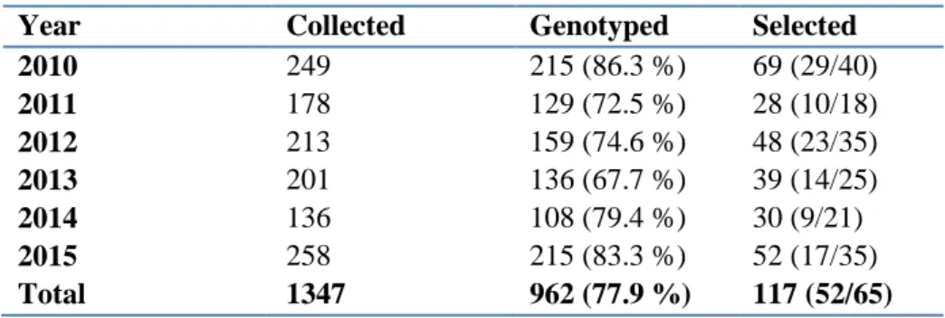
We collected 1347 samples during the 6-years study, of which we excluded 112 (8.3 %) samples missing information on sampling date or location. Not all samples were amplified at the total set of 19 microsatellite loci and we therefore used a subset of 12 loci (ADL142, ADL184, ADL230, BG15, BG16, BG18, LEI098, TuT1, TuT2, TuT3, TuT4 and molecular sexing) shared among all samples. We could determine a reliable genotype in 962 (77.9 %) out of 1235 samples. Genotyping success ranged from 67.7 % (2013) to 86.3 % (2010; Table 2). We estimated rates of genotyping errors from mismatches between replicated genotypes in comparison to a consensus genotypes (Miquel et al. 2006). Rate of allelic dropout ranged from 0.14 (ADL142) to 0.23 (TuT4), and rate of false alleles and PCR artefacts were below 6 %.

The probability that two individuals in the population shared the same multi-locus genotype was low (PI = 1.4 x 10-5_{, PI}

sibs = 5.5 x 10-3), thus suggesting that individuals could be reliably identified by their

multi-locus genotype (Mills et al. 2000). We identified 132 individuals: 59 females, 70 males and three additional individuals for whom sex could not be determined. Numbers of individuals identified annually ranged from 64 (2010) to 33 (2014; Table 2). Most samples (75.9 %) were collected at eleven lek sites and during the breeding season, when 109 individuals were identified, including 61 males and 48 females. The remaining individuals were detected outside of the breeding season or in their wintering ranges and therefore excluded from CMR analyses. For molecular analyses, we analyzed the genetic data from 51 males and 41 females, keeping the individuals with no missing data (i.e. two alleles detected per individuals for all the markers).

Table A2. Number of samples collected per year between 2010 and 2015. 112 samples without information on sampling location or date were excluded. We also indicate annual numbers (and proportion) of samples successfully genotyped, and numbers of individuals (females/males) observed at lekking sites and during the breeding season

Year Collected Genotyped Selected

2010 249 215 (86.3 %) 69 (29/40) 2011 178 129 (72.5 %) 28 (10/18) 2012 213 159 (74.6 %) 48 (23/35) 2013 201 136 (67.7 %) 39 (14/25) 2014 136 108 (79.4 %) 30 (9/21) 2015 258 215 (83.3 %) 52 (17/35) Total 1347 962 (77.9 %) 117 (52/65)

(4)

References

Davison, A. & Chiba, S., 2003. Laboratory temperature variation is a previously unrecognized

source of genotyping error during capillary electrophoresis. Molecular Ecology Notes, 3,

pp.321–323.

Griffiths, R. et al., 1998. A DNA test to sex most birds. Molecular Ecology, 7(8), pp.1071–

1075.

Jacob, G. et al., 2009. Field surveys of capercaillie (Tetrao urogallus) in the Swiss Alps

underestimated local abundance of the species as revealed by genetic analyses of

non-invasive samples. Conservation Genetics, 11(1), pp.33–44.

Kahn, N.W., St John, J. & Quinn, T.W., 1998. Chromosome-specific intron size differences in

the avian CHD gene provide an efficient method for sex identification in birds. Auk,

115(4), pp.1074–1078.

Lefranc, N. & Preiss, F., 2008. Le Grand Tétras Tetrao urogallus dans les Vosges: historique

et statut actuel. Ornithos, 15(4), pp.244–255.

Mills LS, Citta JJ, Lair KP, Schwartz MK, Tallmon DA. 2000. Estimating animal abundance

using noninvasive DNA sampling: promise and pitfalls. Ecological Applications 10:283–

294. Miquel, C. et al., 2006. Quality indexes to assess the reliability of genotypes in studies using

noninvasive sampling and multiple-tube approach. Molecular Ecology Notes, 6(4),

pp.985–988.

Peakall, R. & Smouse, P.E., 2012. GenAlEx 6.5: genetic analysis in Excel. Population genetic

software for teaching and research--an update. Bioinformatics, 28(19), pp.2537–2539.

Piertney, S.B. & Höglund, J., 2001. Polymorphic microsatellite DNA markers in black grouse

(Tetrao tetrix). Molecular Ecology Notes, 1(4), pp.303–304.

Segelbacher, G. et al., 2000. Characterization of microsatellites in capercaillie Tetrao

urogallus (AVES). Molecular Ecology, 9(11), pp.1934–1935.

Taberlet, P. et al., 1996. Reliable genotyping of samples with very low DNA quantities using

PCR. Nucleic Acids Research, 24(16), pp.3189–3194.

(5)

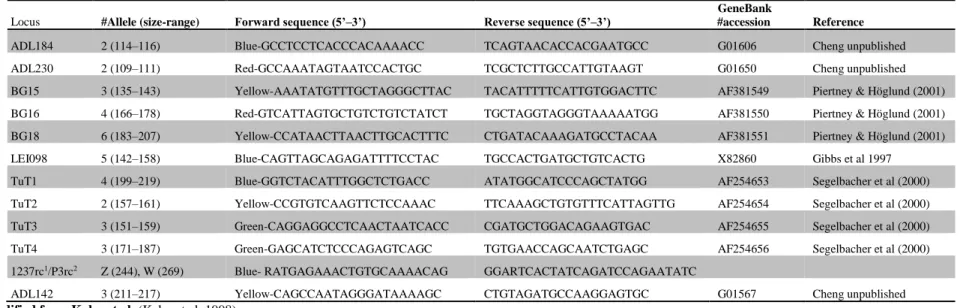
Table A1. Eleven microsatellites and a CHD-gene fragment were amplified in the present study. We indicate locus name, multiplex number, fluorescent dye (Blue: FAM, Yellow: VICTM_{/ATTO 532, Red: PET}TM_{/ATTO 565, Green: NED}TM_{/ATTO 550), number of alleles and allele range, forward and reverse}

sequences, GenBank accession number and reference.

Locus #Allele (size-range) Forward sequence (5’–3’) Reverse sequence (5’–3’)

GeneBank

#accession Reference

ADL184 2 (114–116) Blue-GCCTCCTCACCCACAAAACC TCAGTAACACCACGAATGCC G01606 Cheng unpublished

ADL230 2 (109–111) Red-GCCAAATAGTAATCCACTGC TCGCTCTTGCCATTGTAAGT G01650 Cheng unpublished

BG15 3 (135–143) Yellow-AAATATGTTTGCTAGGGCTTAC TACATTTTTCATTGTGGACTTC AF381549 Piertney & Höglund (2001) BG16 4 (166–178) Red-GTCATTAGTGCTGTCTGTCTATCT TGCTAGGTAGGGTAAAAATGG AF381550 Piertney & Höglund (2001) BG18 6 (183–207) Yellow-CCATAACTTAACTTGCACTTTC CTGATACAAAGATGCCTACAA AF381551 Piertney & Höglund (2001)

LEI098 5 (142–158) Blue-CAGTTAGCAGAGATTTTCCTAC TGCCACTGATGCTGTCACTG X82860 Gibbs et al 1997

TuT1 4 (199–219) Blue-GGTCTACATTTGGCTCTGACC ATATGGCATCCCAGCTATGG AF254653 Segelbacher et al (2000)

TuT2 2 (157–161) Yellow-CCGTGTCAAGTTCTCCAAAC TTCAAAGCTGTGTTTCATTAGTTG AF254654 Segelbacher et al (2000)

TuT3 3 (151–159) Green-CAGGAGGCCTCAACTAATCACC CGATGCTGGACAGAAGTGAC AF254655 Segelbacher et al (2000)

TuT4 3 (171–187) Green-GAGCATCTCCCAGAGTCAGC TGTGAACCAGCAATCTGAGC AF254656 Segelbacher et al (2000)

1237rc1_/P3rc2 _{Z (244), W (269)} _{Blue- RATGAGAAACTGTGCAAAACAG} _{GGARTCACTATCAGATCCAGAATATC}

ADL142 3 (211–217) Yellow-CAGCCAATAGGGATAAAAGC CTGTAGATGCCAAGGAGTGC G01567 Cheng unpublished

1_{modified from Kahn et al. (Kahn et al. 1998)} 2_{modified from Griffiths et al. (Griffiths et al. 1998)}

(6)

APPENDIX B: States and events of Multievent

Capture-Recapture models

Table B1. Quantifying the proportion of dispersers per generation: model states and events

Notation State or event description

States

So Individual with a disperser strategy, stayed in the same lek at t that the one occupied at t–1, and not captured at t

oS+ Individual with a disperser strategy, not captured at t–1, stayed in the same lek at t that the one occupied at t–1, and captured at t

+S+ Individual with a disperser strategy, captured at t–1, stayed in the same lek at t that the one occupied at t–1, and captured at t

Mo Individual with a disperser strategy, moved to another lek between t–1 and t, and not

captured at t

oM+ Individual with a disperser strategy, not captured at t–1, moved to another lek between t–1

and t, and captured at t

+M+ Individual with a disperser strategy, captured at t–1, moved to another lek between t–1 and t,

and captured at t

Ro Individual with a fully resident strategy, stayed in the same lek at t that the one occupied at

t–1, and not captured at t

oR+ Individual with a fully resident strategy, not captured at t–1, stayed in the same lek at t that the one occupied at t–1, and captured at t

+R+ Individual with a fully resident strategy, captured at t–1, stayed in the same lek at t that the one occupied at t–1, and captured at t

D Dead

Events

0 Not captured at t

1 Captured at t, not captured at t–1

2 Captured at t, in the same lek at t that the one occupied at t–1

(7)

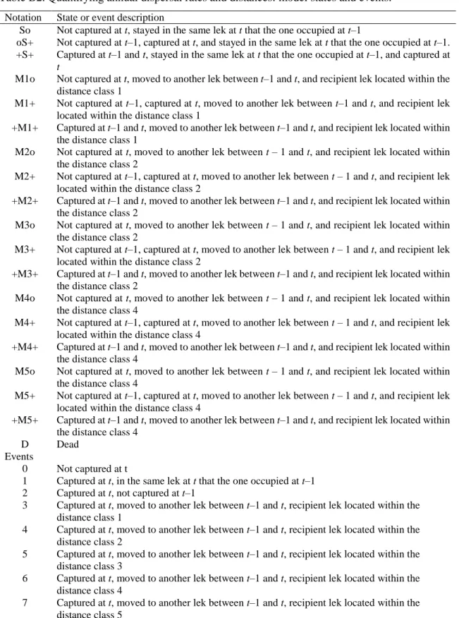
Table B2. Quantifying annual dispersal rates and distances: model states and events.

Notation State or event description

So Not captured at t, stayed in the same lek at t that the one occupied at t–1

oS+ Not captured at t–1, captured at t, and stayed in the same lek at t that the one occupied at t–1. +S+ Captured at t–1 and t, stayed in the same lek at t that the one occupied at t–1, and captured at

t

M1o Not captured at t, moved to another lek between t–1 and t, and recipient lek located within the distance class 1

M1+ Not captured at t–1, captured at t, moved to another lek between t–1 and t, and recipient lek

located within the distance class 1

+M1+ Captured at t–1 and t, moved to another lek between t–1 and t, and recipient lek located within the distance class 1

M2o Not captured at t, moved to another lek between t – 1 and t, and recipient lek located within

the distance class 2

M2+ Not captured at t–1, captured at t, moved to another lek between t – 1 and t, and recipient lek located within the distance class 2

D Dead

Events

0 Not captured at t

1 Captured at t, in the same lek at t that the one occupied at t–1

2 Captured at t, not captured at t–1

3 Captured at t, moved to another lek between t–1 and t, recipient lek located within the

distance class 1

distance class 2

distance class 3

distance class 4

(8)

APPENDIX C: model selection procedure for

capture-recapture analyses

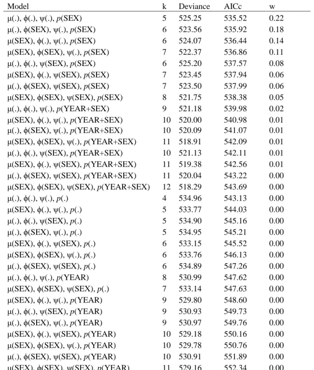
Table C1. Quantifying non-effective dispersal rate per generation: model selection procedure. Model parameters may vary between sexes and years. μ = proportion of dispersers (i.e. individuals that dispersed at least one time during their lifetime) per generation, ϕ = survival probability, ψ = dispersal probability, p = recapture probability, k = number of model parameters, Deviance = residual deviance, AICc = Akaike information criterion adjusted for small sample size, w = AICc weight.

Model k Deviance AICc w

μ(.), ϕ(.), ψ(.), p(SEX) 5 525.25 535.52 0.22

μ(.), ϕ(SEX), ψ(.), p(SEX) 6 523.56 535.92 0.18

μ(SEX), ϕ(.), ψ(.), p(SEX) 6 524.07 536.44 0.14

μ(SEX), ϕ(SEX), ψ(.), p(SEX) 7 522.37 536.86 0.11

μ(.), ϕ(.), ψ(SEX), p(SEX) 6 525.20 537.57 0.08

μ(SEX), ϕ(.), ψ(SEX), p(SEX) 7 523.45 537.94 0.06

μ(.), ϕ(SEX), ψ(SEX), p(SEX) 7 523.50 537.99 0.06

μ(SEX), ϕ(SEX), ψ(SEX), p(SEX) 8 521.75 538.38 0.05

μ(.), ϕ(.), ψ(.), p(YEAR+SEX) 9 521.18 539.98 0.02

μ(SEX), ϕ(.), ψ(.), p(YEAR+SEX) 10 520.00 540.98 0.01 μ(.), ϕ(SEX), ψ(.), p(YEAR+SEX) 10 520.09 541.07 0.01 μ(SEX), ϕ(SEX), ψ(.), p(YEAR+SEX) 11 518.91 542.09 0.01 μ(.), ϕ(.), ψ(SEX), p(YEAR+SEX) 10 521.13 542.11 0.01 μ(SEX), ϕ(.), ψ(SEX), p(YEAR+SEX) 11 519.38 542.56 0.01 μ(.), ϕ(SEX), ψ(SEX), p(YEAR+SEX) 11 520.04 543.22 0.00 μ(SEX), ϕ(SEX), ψ(SEX), p(YEAR+SEX) 12 518.29 543.69 0.00

μ(.), ϕ(.), ψ(.), p(.) 4 534.96 543.13 0.00 μ(SEX), ϕ(.), ψ(.), p(.) 5 533.77 544.03 0.00 μ(.), ϕ(.), ψ(SEX), p(.) 5 534.90 545.16 0.00 μ(.), ϕ(SEX), ψ(.), p(.) 5 534.95 545.21 0.00 μ(SEX), ϕ(.), ψ(SEX), p(.) 6 533.15 545.52 0.00 μ(SEX), ϕ(SEX), ψ(.), p(.) 6 533.76 546.13 0.00 μ(.), ϕ(SEX), ψ(SEX), p(.) 6 534.89 547.26 0.00 μ(.), ϕ(.), ψ(.), p(YEAR) 8 530.99 547.62 0.00

μ(SEX), ϕ(SEX), ψ(SEX), p(.) 7 533.14 547.63 0.00

μ(SEX), ϕ(.), ψ(.), p(YEAR) 9 529.80 548.60 0.00

μ(.), ϕ(.), ψ(SEX), p(YEAR) 9 530.93 549.73 0.00

μ(.), ϕ(SEX), ψ(.), p(YEAR) 9 530.97 549.76 0.00

μ(SEX), ϕ(.), ψ(SEX), p(YEAR) 10 529.18 550.16 0.00 μ(SEX), ϕ(SEX), ψ(.), p(YEAR) 10 529.78 550.76 0.00 μ(.), ϕ(SEX), ψ(SEX), p(YEAR) 10 530.91 551.89 0.00 μ(SEX), ϕ(SEX), ψ(SEX), p(YEAR) 11 529.16 552.34 0.00

(9)

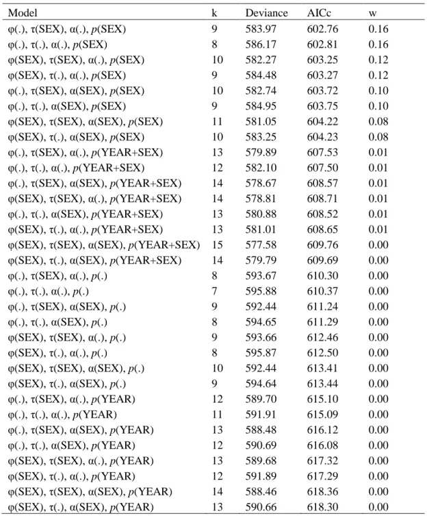
Table C2. Quantifying non-effective annual dispersal rates and distances: model selection procedure. Model parameters may vary between sexes and years. ϕ = survival probability, τ = departure probability, α = arrival probability, p = recapture probability, k = number of model parameters, Deviance = residual deviance, AICc = Akaike information criterion adjusted for small sample size, w = AICc weight.

Model k Deviance AICc w

φ(.), τ(SEX), α(.), p(SEX) 9 583.97 602.76 0.16

φ(.), τ(.), α(.), p(SEX) 8 586.17 602.81 0.16

φ(SEX), τ(SEX), α(.), p(SEX) 10 582.27 603.25 0.12

φ(SEX), τ(.), α(.), p(SEX) 9 584.48 603.27 0.12

φ(.), τ(SEX), α(SEX), p(SEX) 10 582.74 603.72 0.10

φ(.), τ(.), α(SEX), p(SEX) 9 584.95 603.75 0.10

φ(SEX), τ(SEX), α(SEX), p(SEX) 11 581.05 604.22 0.08

φ(SEX), τ(.), α(SEX), p(SEX) 10 583.25 604.23 0.08

φ(.), τ(SEX), α(.), p(YEAR+SEX) 13 579.89 607.53 0.01 φ(.), τ(.), α(.), p(YEAR+SEX) 12 582.10 607.50 0.01 φ(.), τ(SEX), α(SEX), p(YEAR+SEX) 14 578.67 608.57 0.01 φ(SEX), τ(SEX), α(.), p(YEAR+SEX) 14 578.81 608.71 0.01 φ(.), τ(.), α(SEX), p(YEAR+SEX) 13 580.88 608.52 0.01 φ(SEX), τ(.), α(.), p(YEAR+SEX) 13 581.01 608.65 0.01 φ(SEX), τ(SEX), α(SEX), p(YEAR+SEX) 15 577.58 609.76 0.00 φ(SEX), τ(.), α(SEX), p(YEAR+SEX) 14 579.79 609.69 0.00

φ(.), τ(SEX), α(.), p(.) 8 593.67 610.30 0.00 φ(.), τ(.), α(.), p(.) 7 595.88 610.37 0.00 φ(.), τ(SEX), α(SEX), p(.) 9 592.44 611.24 0.00 φ(.), τ(.), α(SEX), p(.) 8 594.65 611.29 0.00 φ(SEX), τ(SEX), α(.), p(.) 9 593.66 612.46 0.00 φ(SEX), τ(.), α(.), p(.) 8 595.87 612.50 0.00

φ(SEX), τ(SEX), α(SEX), p(.) 10 592.44 613.41 0.00

φ(SEX), τ(.), α(SEX), p(.) 9 594.64 613.44 0.00

φ(.), τ(SEX), α(.), p(YEAR) 12 589.70 615.10 0.00

φ(.), τ(.), α(.), p(YEAR) 11 591.91 615.09 0.00

φ(.), τ(SEX), α(SEX), p(YEAR) 13 588.48 616.12 0.00

φ(.), τ(.), α(SEX), p(YEAR) 12 590.69 616.08 0.00

φ(SEX), τ(SEX), α(.), p(YEAR) 13 589.68 617.32 0.00

φ(SEX), τ(.), α(.), p(YEAR) 12 591.89 617.29 0.00

φ(SEX), τ(SEX), α(SEX), p(YEAR) 14 588.46 618.36 0.00 φ(SEX), τ(.), α(SEX), p(YEAR) 13 590.66 618.30 0.00

(10)

Yearly-specific dispersal rates in the population of Western capercaillie (Tetrao urogallus).

We examined how departure rate fluctuated between years by comparing the AICc of the two following models, (φ(.), τ(.), α(.), p(SEX)) and (φ(.), τ(YEAR), α(.), p(SEX)). In the first model, departure rate was hold constant (τ(.)) whereas it varied between years in the second model (τ(YEAR)). The model in which departure was hold constant was better supported by the data (AICc = 602.81) than the model with a year effect (AICc = 605.48). This result indicates lowly variable departure rates between years (see Figure C1).

Figure C1. Yearly-specific dispersal rates in the population of Western capercaillie (Tetrao

urogallus). We show yearly-specific departure rates and their 95% CI extracted from the model

(φ(.), τ(YEAR), α(.), p(SEX)). The red line corresponds to constant departure rate extracted from the model (φ(.), τ(.), α(.), p(SEX)).

(11)

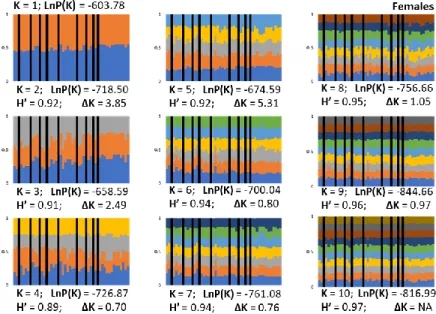
APPENDIX D: Population genetic structure

Fig. D1. STRUCTURE outputs for all the individuals (males and females).

(12)

Fig. D3. STRUCTURE outputs for females only.

(13)

Fig. D5. DAPC for females only.

Table D1. Results of the simulations performed in CO-ANCESTRY. Our analyses revealed that the estimator LynchRd (shown in grey) was the most accurate for our dataset.

TrioML Wang LynchLi LynchRd Ritland QuellerGt DyadML True Value

Mean 0,26 0,22 0,22 0,22 0,21 0,21 0,3 0,23

Variance 0,05 0,12 0,12 0,1 0,15 0,11 0,06 0,04

MSE 0,04 0,08 0,08 0,06 0,12 0,07 0,04 NA

(14)

APPENDIX E: Influence of landscape predictors on genetic

variation

A. Details on landscape predictors.

Dtopo was computed as the cumulated length of segments that would be travelled by an individual

flying in straight line from a point A to a point B while following topographic relief. From a Digital Elevation Model (DEM) at a 25m resolution, we computed the effective travelled distance d across each pixel i crossed by an individual along its straight line trajectory using the Pythagorean Theorem as follows: 𝑑𝑖 = √(𝑥𝑖−1− 𝑥𝑖)2+ (𝑦𝑖−1− 𝑦𝑖)2 , with (𝑥𝑖−1− 𝑥𝑖) = 25 (the length of a pixel), 𝑦𝑖−1 the altitude at the previous pixel along the trajectory and 𝑦𝑖 the altitude at the focal pixel. Dtopo was then computed as the sum of distances 𝑑𝑖 along the trajectory.

To compute Dslope, we first created a slope raster map at a 25m resolution from the DEM using the Spatial Analyst toolbox in ArcGis 10.2. The layer was rescaled to range from 1 to 100 and we used CIRCUITSCAPE 3.5.8 to compute pairwise effective distances between individual locations, with the raster coded in resistances (higher slope values denoting greater resistance to movement).

To compute Dridge, we first applied the Focal Statistics tool from the Spatial Analyst toolbox to compute, for each pixel from the DEM, the mean elevation values within a 1000m neighborhood. We then subtracted the Focal Stats layer from the original DEM and identified ridges as pixels associated with a positive value (pixels above the average elevation of their neighborhood). Altitude values of ridge pixels were rescaled to range from 1(highest elevation) to 100 (lowest elevation) whereas non-ridge pixels were systematically set to 100. We finally used CIRCUITSCAPE 3.5.8 to compute pairwise effective distances between individual locations, with the raster coded in resistances (non-ridge areas denoting greater resistance to movement).

B. Identification of the main contributors to the variance in pairwise measures of genetic differentiation.

We coupled multiple linear regressions on standardized data at the optimal scale of analysis (see main text for details) with commonality analyses (CA; Ray-Murkherjee et al. 2014) to identify the main contributors to the variance in the dependent variable Rxy after sequential removing of suppressors and unnecessary predictors. Predictors were identified as suppressors when their unique contribution was (almost) totally counterbalanced by a negative commonality coefficient (classical and reciprocal suppression) or when standardized regression coefficients and structure coefficients were of opposite signs (cross-over suppression; Paulhus et al. 2004, Prunier et al. 2017). Predictors were identified as unnecessary when their unique contribution (U) was null (or when the lower bound of 95 % confidence intervals CI around U was null), indicating that they only contributed to the variance in the dependent variable because of their synergistic association with one or several other predictors (Prunier et al., 2015). The 95 % CI around beta coefficients β and unique contributions U were computed from bootstrap resampling (1000 iterations).

For each sex (M and F), the following table provides details about runs of identification of unnecessary predictors (in synergistic association with other predictors) and suppressors in full models (see main text for details). Are provided: typical results of the different runs of multiple linear regressions (model fit R², predictors Pred, structure coefficients rs and standardized coefficients β),

(15)

along with additional parameters derived from CA: unique, common and total contributions of predictors to the variance in dependent variable (U, C and T), as well as 95% confidence intervals about U (UCIlow and UCIup) as computed from bootstrap (1000 iterations). The rationale for

withdrawal of predictors (Ra) is the following: S: synergistic association with other predictors (UCIlow

= 0); CO: Cross-over suppression. In bold: parameters allowing the identification of unnecessary predictors and suppressors.

In each sex, the main contributor to the variance in measures of genetic dissimilarity was the topographic distance (Dtopo). Results were similar when considering Bc and Dps measures of genetic dissimilarity (data not shown).

Sex Run R² Pred rs β Unique UCIlow UCIup Common Total %U Ra

M 1 0.355 ED 0.958 0.179 0.004 0.000 0.016 0.322 0.326 0.011 S Dtopo 0.954 0.304 0.024 0.010 0.043 0.299 0.323 0.068 Dridge 0.891 0.098 0.002 0.000 0.014 0.280 0.282 0.005 S Dslope 0.681 0.068 0.003 0.000 0.014 0.162 0.165 0.008 S 2 0.323 Dtopo 0.568 0.568 / / / / / / F 1 0.076 ED 0.927 0.042 0.000 0.000 0.007 0.065 0.065 0.003 S Dtopo 0.993 0.257 0.011 0.002 0.028 0.064 0.075 0.140 Dridge 0.805 -0.048 0.001 0.000 0.009 0.049 0.049 0.007 S and CO Dslope 0.547 0.037 0.001 0.000 0.008 0.022 0.023 0.008 S 2 0.075 Dtopo 0.273 0.273 / / / / / / References

Ray‐ Mukherjee, J., Nimon, K., Mukherjee, S., Morris, D. W., Slotow, R., & Hamer, M. (2014). Using commonality analysis in multiple regressions: a tool to decompose regression effects in the face of multicollinearity. Methods in Ecology and Evolution, 5, 320-328.

Paulhus, D. L., Robins, R. W., Trzesniewski, K. H., & Tracy, J. L. (2004). Two replicable suppressor situations in personality research. Multivariate Behavioral Research, 39, 303-328.

Prunier, J. G., Colyn, M., Legendre, X., Nimon, K. F., & Flamand, M. C. (2015). Multicollinearity in spatial genetics: separating the wheat from the chaff using commonality analyses. Molecular Ecology, 24, 263-283.

Prunier, J. G., Colyn, M., Legendre, X., & Flamand, M. C. (2017). Regression commonality analyses on hierarchical genetic distances. Ecography, 40, 1412-1425.

(16)

APPENDIX F: Relatedness effect on first capture and departure

Fig. F1. Distribution of the mean of average relatedness within lek. Left: males only; Right: females only; Top: permutated first capture; Bottom: permutated departure. Red dash lines represent original dataset values.