HAL Id: hal-02946565
https://hal.archives-ouvertes.fr/hal-02946565
Submitted on 23 Sep 2020
HAL is a multi-disciplinary open access
archive for the deposit and dissemination of
sci-entific research documents, whether they are
pub-lished or not. The documents may come from
teaching and research institutions in France or
abroad, or from public or private research centers.
L’archive ouverte pluridisciplinaire HAL, est
destinée au dépôt et à la diffusion de documents
scientifiques de niveau recherche, publiés ou non,
émanant des établissements d’enseignement et de
recherche français ou étrangers, des laboratoires
publics ou privés.
Relaxation-Aware Heuristics for Exact Optimization in
Graphical Models
Fulya Trösser, Simon De Givry, George Katsirelos
To cite this version:
Fulya Trösser, Simon De Givry, George Katsirelos. Relaxation-Aware Heuristics for Exact
Optimiza-tion in Graphical Models. CPAIOR 2020: SEVENTEENTH INTERNATIONAL CONFERENCE
ON THE INTEGRATION OF CONSTRAINT PROGRAMMING, ARTIFICIAL INTELLIGENCE,
AND OPERATIONS RESEARCH, Sep 2020, Vienna, Austria. �10.1007/978-3-030-58942-4_31�.
�hal-02946565�
Optimization in Graphical Models
Fulya Tr¨osser1, Simon de Givry1a, and George Katsirelos2b 1
MIAT, UR-875, INRAE, F-31320 Castanet Tolosan, France {fulya.ural,simon.de-givry}@inrae.fr -a
ORCiD: 0000-0002-2242-0458
2 UMR MIA-Paris, INRAE, AgroParisTech, Univ. Paris-Saclay, 75005 Paris, France
[email protected] -bORCiD: 0000-0002-3727-6698
Abstract. Exact solvers for optimization problems on graphical models, such as Cost Function Networks and Markov Random Fields, typically use branch-and-bound. The efficiency of the search relies mainly on two factors: the quality of the bound computed at each node of the branch-and-bound tree and the branching heuristics. In this respect, there is a trade-off between quality of the bound and computational cost. In par-ticular, the Virtual Arc Consistency (VAC) algorithm computes high quality bounds but at a significant cost, so it is mostly used in prepro-cessing, rather than in every node of the search tree.
In this work, we identify a weakness in the use of VAC in branch-and-bound solvers, namely that they ignore the information that VAC pro-duces on the linear relaxation of the problem, except for the dual bound. In particular, the branching heuristic may make decisions that are clearly ineffective in light of this information. By eliminating these ineffective decisions, we significantly reduce the size of the branch-and-bound tree. Moreover, we can optimistically assume that the relaxation is mostly cor-rect in the assignments it makes, which helps find high quality solutions quickly. The combination of these methods shows great performance in some families of instances, outperforming the previous state of the art. Keywords: Graphical model · Cost function network · Weighted con-straint satisfaction problem · Virtual arc consistency · Branch-and-bound · Linear relaxation · Local polytope · Variable ordering heuristic.
1
Introduction
Undirected graphical models like Cost Function Networks, aka Weighted Con-straint Satisfaction Problems (WCSP), and Markov Random Fields (MRF) can be used to give a factorized representation of a function, in which vertices of a graph represent variables of the function and (hyper)edges represent factors. The factors can be, for example, cost functions, in which case the graphical model represents a factorization of a cost function, or local probability tables, in which case the model represents a non-normalized joint probability distribution [17].
0
Some supplementary figures available at genoweb.toulouse.inra.fr/~degivry/ evalgm/TrosserCPAIOR20supp.pdf
The two models, WCSP and MRF, are equivalent under a − log transfor-mation, hence the NP-complete cost minimization query in WCSP is equivalent to the maximum a posteriori (MAP) assignment query in MRF. This optimiza-tion problem has applicaoptimiza-tions in many areas, such as image analysis, speech recognition, bioinformatics, and ecology.
Exact solution methods for this problem are mostly based on branch-and-bound. For example, one can express WCSP optimization as an integer linear program (ILP) and use a solver for that problem. However, ILP solvers need to solve the linear relaxation of the instance exactly to obtain a bound at each node of the branch-and-bound tree, an operation that is too expensive for the scale of problems encountered in many applications. Instead, the most success-ful dedicated solvers use algorithms that in effect solve the linear relaxation approximately and therefore potentially suboptimally. Specifically, algorithms like EDAC [9], VAC [6], TRWS [18] and others, produce feasible solutions to the dual of the linear relaxation of the WCSP, which can be used as lower bounds. For the loss of precision that they give up, these algorithms gain significantly in computational efficiency. In stark contrast to integer programming, not only is exact LP solving not used, but the preferred method for branch-and-bound, EDAC, is by far the weakest, while VAC or TRWS are most often used only in preprocessing.
There are a few exceptions to the norm of using branch-and-bound for this problem: core-guided MaxSAT solvers [21], logic-based Benders decomposition [8], cut generation [24], to name a few. Here, we are interested in the CombiLP method [13], which solves the linear relaxation and decomposes the problem into two parts: the “easy” part which corresponds to the set of integral variables in the linear relaxation and a combinatorial part which contains the variables assigned fractional values. They then proceed to solve the combinatorial subset exactly and if that solution can be combined with the easy part without incurring extra cost, it reports optimality. Otherwise, it moves some variables from the easy part to the combinatorial part and iterates. Crucially, they identify integral variables by identifying a condition called Strict Arc Consistency (Strict AC) on the dual solution produced, and can therefore be used with approximate dual LP solvers, like VAC and TRWS, which may produce a suboptimal dual LP solution for which no corresponding primal solution exists.
We make several contributions here. First, we relax Strict AC, the condition that CombiLP uses to detect integrality. We show in Section 3 that the relaxed condition admits larger sets of integral variables. Second, we show that a class of fixpoints of an LP solver like VAC implies a specific set of integral variables regardless of the dual solution it finds, even when those variables do not satisfy the Strict AC condition in this solution. This avoids the need to bias the LP solver towards solutions that contain Strict AC variables. On the practical side, we introduce two simple techniques that exploit this property within a branch-and-bound solver. The first, given in Section 5 modifies the branching heuristic to avoid branching on Strict AC variables, as that is unlikely to be informative. The second, given in Section 6, is a variant of the well-known RINS heuristic in
integer programming ([7]), which optimistically assumes that the set of Strict AC variables assigned their integral values actually appear in the optimal so-lution and solves a restricted sub-problem to help quickly identify high quality solutions. In Section 7, we show that integrating these techniques in the toul-bar2 solver [6] improves performance significantly over the state of the art in some families of instances.
2
Preliminaries
Definition 1. A Constraint Satisfaction Problem (CSP) [6] is a triple hX, D, Ci. X is a set of n variables X = {1, . . . , n}. Each variable i ∈ X has a domain of values Di ∈ D and can be assigned any value a ∈ Di, also noted (i, a). C is
a set of constraints. Each constraint cS ∈ C is defined over a set of variables
S ⊆ X (called the scope of the constraint) by a subset of the Cartesian product Q
i∈SDi which defines all consistent tuples of values.
We assume, without loss of generality, that at most one constraint is defined over a given set of variables. The unary constraint on variable i will be denoted ci, and binary constraints cij. The cardinality |S| is the arity of cS. For J ⊆ X,
`(J ) denotes the set of all possible tuples for J , i.e., `(J ) =Q
i∈JDi. Let S ⊆ X,
and t ∈ `(S), the projection of t onto V ⊆ S is denoted by t[V ]. A tuple t satisfies a constraint cS if t[S] ∈ cS. A tuple t ∈ `(X) is a solution iff it satisfies all the
constraints in C. Finding a solution is NP-complete.
Definition 2. A Weighted Constraint Satisfaction Problem (WCSP) [6] is a quadruple hX, D, C, ki where X is a set of n variables X = {1, . . . , n}, each variable i ∈ X has a domain of possible values Di∈ D, as in CSP. C is a set of
cost functions, and k is a positive integer or infinity serving as the upper bound. Each cost function hS, cSi ∈ C is defined over a set of variables S ⊆ X (its scope)
and cS maps each assignment to the variables in S to non-negative integer costs.
WCSPs generalize CSPs as they can represent the same set of feasible solu-tions with infinite cost cS(t) = k for forbidden tuples t, but additionally define a
cost for feasible assignments. We assume all WCSPs contain a unary cost func-tion for each variable and a cost funcfunc-tion c∅, which represents a constant in the
objective function. Since all costs are non-negative, c∅ is a lower bound on the
cost of feasible solutions of the WCSP.
If the largest arity of any cost function in a WCSP is 2, then we say this is a binary WCSP. We focus on binary WCSPs here, both for simplicity and because of technical limitations of the implementation. However, all definitions and properties we present can easily be generalized to higher arities.
A binary WCSP can be graphically represented as shown in Fig. 1a. Each variable i ∈ X corresponds to a cell. Each value a ∈ Di corresponds to a dot in
the cell. A unary cost ci(a) is written next to the dot only if it is non-zero. If
there is a non-zero binary cost between (i, a) and (j, b), then an edge is drawn between the dots corresponding to these assignments.
The problem is to find a solution t ∈ `(X) which minimizes the sum of all cost functions, denoted as cP(t) = c∅+Pi∈Xci(t[i]) +Pcij∈Ccij(t[i], t[j]), and
such that cP(t) < k. This is denoted opt(P ). This problem is NP-hard.
Given two WCSPs P , P0 with the same set of variables and scopes, we say they have the same structure. If cP(t) = cP0(t) for all t ∈ l(X) then P and P0
are equivalent and they are reparameterizations of each other. It has been shown [6] that the optimal reparameterization, which maximizes the constant factor in the objective, is given by the dual of the following linear program (LP), called the local polytope of the WCSP:
min c∅+ X i∈X,a∈Di ci(a)xia+ X cij∈C,a∈Di,b∈Dj
cij(a, b)yiajb
s.t. X a∈Di xia= 1 ∀i ∈ X xia= X b∈Dj yiajb ∀i ∈ X, a ∈ Di, cij ∈ C 0 ≤ xia≤ 1 ∀i ∈ X, a ∈ Di 0 ≤ yiajb≤ 1 ∀cij ∈ C, a ∈ Di, b ∈ Dj (1) From the optimal solution of the above LP, the reparameterization is ex-tracted from the reduced costs r(xia) and r(yiajb) of each variable and binary
cost function, respectively, by setting ci(a) to r(xia) and cij(a, b) to r(yiajb) and
setting c∅to the optimum of the LP (1). Because of the correspondence between
reparameterizations and solutions of this LP, we use the two interchangeably. In this paper, we work with algorithms that do not solve this LP exactly but compute a feasible solution of its dual. In particular, the VAC algorithm computes a reformulation which is virtual arc consistent (VAC), as defined below. Definition 3. A CSP P is arc consistent (AC) if for all cij ∈ C, ∀a ∈ Di,
∃b ∈ Dj with {(i, a), (j, b)} ∈ cij, and ∀b ∈ Dj, ∃a ∈ Diwith {(i, a), (j, b)} ∈ cij.
The arc consistent closure AC(P ) is the unique CSP which results from removing values from domains that violate the arc consistency property.
The CSP AC(P ) is equivalent to P , i.e., it has exactly the same set of solu-tions. In particular, if AC(P ) is empty (has empty domains), P is unsatisfiable. Definition 4 ([6]). Let P = hX, D, C, ki be a WCSP. Then Bool(P ) = hX, D, Ci (Boolθ(P ) = hX, Dθ, Cθi) is the CSP where, for all i ∈ X, a ∈ Di (resp. Dθi)
if and only if ci(a) = 0 (resp. ci(a) < θ) and for all i, j ∈ X2, h{i, j}, Riji ∈ C
(resp. Cθ) iff ∃cij ∈ C, where Rij is the relation ∀a ∈ Di (resp. Dθi), ∀b ∈ Dj
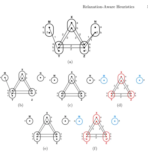
X Y Z M N a a a a a b b b b b c c 2 2 2 2 2 2 1 1 1 2 2 1 (a) X Y Z M N a a a a a b b b c (b) X Y Z M N a a a a a b b b (c) X Y Z M N a a a a a b b b 2 2 2 2 2 2 (d) X Y Z M N a a a a a b b b c c (e) 1 X Y Z M N a a a a a b b b c c 2 2 2 2 2 2 1 (f)
Fig. 1: Stratified VAC and RASPS examples for two different thresholds. Blue vari-ables are VAC-integral. (a) A WCSP instance P with 5 varivari-ables {M, X, Y, Z, N }. (b) Bool1(P ) = Bool(P ) (c) AC(Bool1(P )). (d) WCSP instance P1 constructed
by RASPS from AC(Bool1(P )). Optimal solution is {a, a, b, a, a} with cost 2. (e)
Bool2(P ) = AC(Bool2(P )). (f) WCSP instance P2 constructed by RASPS from
AC(Bool2(P )). Optimal solution is {a, a, b, c, a} with cost 1, optimum of P .
By construction, Bool(P ) admits exactly the solutions of P with cost c∅, since
all assignments that have non-zero cost in any cost function of P are mapped to forbidden tuples in Bool(P ). Thus, if Bool(P ) is unsatisfiable, c∅ < opt(P ).
There is no such clear result for Boolθ(P ), but it is useful in practice. Examples
of Boolθ(P ) are shown in Fig. 1b, 1e where edges correspond to forbidden tuples.
Definition 5. A WCSP P is virtual arc consistent (VAC) if the arc consistency closure of the CSP Bool(P ) is non-empty [6].
If AC(Bool(P )) is empty, then Bool(P ) is unsatisfiable and hence c∅ <
Opt(P ). The VAC algorithm iteratively computes whether AC(Bool(P )) is empty and if so extracts a reparameterization which provably improves the lower bound c∅. It terminates when AC(Bool(P )) is non-empty. It converges to a non-unique
fixpoint which may not match the LP optimum. Conversely, the reparameteri-zation given by the dual optimal solution is VAC.
In the following, we assume mint∈`(S)cS(t) = 0 for all scopes S. Otherwise,
the instance can be trivially reparameterized to increase the lower bound.
3
Strict Arc Consistency and VAC-integrality
Savchynskyy et al. introduced Strict Arc Consistency ([23]) as a way to partition a WCSP into an “easy” part, which can be solved exactly by an LP solver and a “hard” combinatorial part.
Definition 6 (Strict Arc Consistency [23]). A variable i ∈ X is Strictly Arc Consistent if there exists a unique value a ∈ Di such that ci(a) = 0 and a
unique tuple {(i, a), (j, b)} which satisfies cij(a, b) = 0 ∀cij∈ C. The value a is
called the Strict AC value of i.
Given a WCSP P and a subset S of its variables such that all variables in S are Strict AC, we can solve P restricted to S exactly by assigning the Strict AC value to each variable. This property gives a natural partition of a WCSP into the set of Strict AC variables and the rest. This partition was used by Savchynskyy et al. [23] and in a refined algorithm introduced later [13]. These algorithms exploit the solvability of the Strict AC subset of variables and only need to solve the smaller non-Strict-AC subset using a combinatorial solver.
Our first contribution here is to note that the Strict AC property is stronger than necessary3. In particular, we can weaken the second condition as follows: Definition 7 (VAC-integrality). A variable i ∈ X is VAC-integral if there ex-ists a unique value a ∈ Disuch that ci(a) = 0 and at least one tuple {(i, a), (j, b)}
which satisfies cij(a, b) + cj(b) = 0 ∀cij ∈ C. The value a is the VAC-integral
value of x.
The difference between VAC-integrality and Strict AC is that in VAC-integrality, the second condition requires that the witness value appears in at least one rather than exactly one 0-cost tuple in each incident constraint. The VAC-integral sub-set of a WCSP maintains the main property of Strict AC, namely that it is exactly solvable by inspection and its optimal solution has cost 0. The opti-mal solution, as in Strict AC, simply assigns to each VAC-integral variable its VAC-integral value. By definition, this has cost 0.
Since VAC-integrality is a relaxation of Strict AC, every Strict AC set of variables is also VAC-integral. The inverse does not hold (see Supplementary Fig. 1). However, this only holds for instances that are at a VAC fixpoint. Proposition 1. If a WCSP instance P is VAC and a variable i is strict AC then it is also VAC-integral.
3 We also change the name of the property from “consistency”, which implies an
algorithm that achieves said consistency, to “integrality”. Adding the VAC term will become clear after Proposition 3.
As with Strict AC, VAC-integrality implies integrality of the corresponding primal solution by complementary slackness.
Proposition 2. The VAC-integral variables in an optimal dual solution of (1) correspond to the variables i for which there exists a unique a with xia= 1 and
xib= 0 for b 6= a in the corresponding optimal primal solution.
Proof (Sketch). Given an optimal dual solution of the local polytope LP, for each VAC-integral variable i with VAC-integral value a, the primal solution must have xib= 0 for all b 6= a by complementary slackness and hence xia= 1. ut
Note that in the case of approximate dual LP solvers like VAC and TRWS, this observation does not hold: if the dual solution is not optimal, there is no primal solution with the same cost. Rather, we use Strict AC and VAC-integrality as proxies for conditions which would lead to integrality in optimal solutions, while maintaining the property that they admit zero cost solutions.
One complication with both Strict AC and VAC-integrality is that any lower bound given by a dual solution can in fact be produced by several dual solutions, but they do not all give the same VAC-integrality subset. One way to deal with this is to bias the LP solver towards solutions that maximize the VAC-integral subset [13]. Here we propose another method, given by the following observation. Proposition 3. Given a WCSP instance P which is VAC and a variable i, if in AC(Bool(P )) it holds that Di = {a} then i is VAC-integral with value a.
Proof (Sketch). Since AC(Bool(P )) is arc consistent, if a value remains in the domain of i in Bool(P ), it has unary cost 0 in P and is supported by tuples and values of cost 0 in all incident constraints. Conversely, if a value is removed in Bool(P ), either it has non-zero unary cost in P or some non-zero amount of cost
can be moved onto it [6]. ut
The effect of Proposition 3 is that the class of dual feasible solutions which have the same AC(Bool(P )) produce the same set of VAC-integral variables, even though most of these solutions do not satisfy Definition 7. This is shown in in the WCSP of figure 1a which is VAC but only variable N is VAC-integral. However, by applying Proposition 3, we get from AC(Bool(P )) that M is also VAC-integral. Therefore, this observation allows us to construct a larger VAC-integral subset than that given by collecting the variables that satisfy the VAC-integrality property given a dual solution. This has the advantage that we do not need to modify the LP solver to be biased towards specific dual solutions and is easy to use with VAC, which explicitly maintains Bool(P ). We can apply the same reasoning to find Strict AC sets of variables, using the following condition. Proposition 4. If a WCSP instance P is VAC, then a VAC-integral variable i is strict AC if and only if all its neighbors are VAC-integral.
Complexity. It is natural to ask whether the presence of a large VAC-integral sub-set makes the problem easier to solve, in the sense of fixed parameter tractabil-ity [11]. Unfortunately, this turns out not to be the case. Let Almost-Integral-WCSP be the class of WCSPs which are VAC with n − 1 VAC-integral variables. We show that it is NP-complete, which implies that WCSP is para-NP-complete for the parameter of number of non-VAC-integral variables.
Theorem 1. Almost-Integral-WCSP is NP-Complete.
Proof. Membership in NP is obvious since this is a subclass of WCSP. For hard-ness, we reduce from binary WCSP. Let P = hX, D, C, ki be an arbitrary WCSP instance and assume that it is VAC. We construct P0= hX ∪ X0∪ {q}, D, C0, k +
|C|i, where X0 is a copy of the variables in X, including the unary cost
func-tions and q has domain {a, b} with cq(a) = cq(b) = 0. For each cost function with
scope {i, j} in C, P0 has two cost functions with scopes {i, j, q} and {i0, j0, q}.
Each variable in P has at least one value with unary cost 0, since it is VAC. Let this value be a for all variables. We define the ternary cost functions to be cijq(a, a, a) = 0, cijq(u, v, a) = k when u 6= a or v 6= a, cijq(u, v, b) = cij(u, v) + 1
for all u, v. Similarly, ci0j0q(a, a, b) = 0, ci0j0q(u, v, b) = k when u 6= a or v 6= a,
ci0j0q(u, v, a) = cij(u, v) + 1 for all u, v.
P0is an instance of Almost-Integral-WCSP with q the non-VAC-integral variable. Indeed, ci(a) = 0 for all variables i ∈ X ∪ X0and it is supported by the
zero cost tuple (a, a, a) in each ternary constraint. All other values appear only in ternary tuples with non-zero cost hence will be pruned in AC(Bool(P0)).
P has optimum solution of cost c if and only if P0has optimum of cost c+|C|. Indeed, when we assign q to a or b, the problem is decomposed into independent binary WCSPs on X and X0. One of these admits the all-a, 0-cost assignment and the other is identical to P with an extra cost of 1 per cost function. ut Although this construction uses ternary cost functions, we can convert them to binary using the hidden encoding [4]. This preserves arc consistency, hence it also preserves VAC, so the result holds also for binary WCSPs.
4
Stratified VAC
The foundation of all the heuristics we present in this paper is the implemen-tation of VAC in toulbar2 [6], which is restricted to binary WCSPs. In this implementation, the non-zero binary costs cij(a, b) are stratified. Specifically,
they are sorted in decreasing order and placed in a fixed number l of buckets. The minimum cost θiof each bucket i ∈ {1, . . . , l} defines a sequence of
thresh-olds (θ1, . . . , θl). At each θi for i from 1 to l, it constructs the Boolθi(P ) and
iterates on it until no domain wipe-out occurs. After θl, it follows a geometric
schedule θi+1=θ2i until θi= 1. The reader is referred to [6] for more details.
For a smaller θi, Boolθi(P ) is more restricted, i.e. the domain sizes are
re-duced. The overall, informal observation is that the set of VAC-integral variables expands as θi gets smaller, and saturates at some point, which is usually before
θi= 1. However, even after this saturation, the domain sizes of non-VAC-integral
variables do not necessarily cease shrinking. For the heuristic we present in Sec-tion 6, we aim to choose a threshold θ where we have a good compromise between the number of VAC-integral variables and the domain sizes of non-VAC-integral variables. This way, we increase the size of the easy (VAC-integral) part and de-crease the complexity of the difficult part, while hopefully keeping most (may-be all) values belonging to the optimal solution (see Fig. 1d and 1f). In an informal sense, we consider those VAC-integral variables that were present with a higher θ to be more informative, and more likely to appear in an optimal solution. For example, if we assign against the VAC-integral value for a high value θi, the cost
of the best possible solution is at least c∅+ θi, whereas for θi0 = 1, the cost of
the best possible solution that disagrees with the VAC-integral value can only be shown to be c∅+ 1. Thus, the higher the θ for which a variable is VAC-integral,
the less tight the relaxation needs to be for the corresponding VAC-integral value to appear in an optimal solution.
5
Branching Heuristics based on VAC-integrality
For a branch-and-bound algorithm, the order in which variables are assigned has a crucial impact on the performance. In general, a branching decision should help the solver quickly prune sub-trees which contain no improving solutions, by creating sub-problems with increased dual bound in all branches [1].
Based on this observation and the connection of VAC-integrality to integrality explained in Section 3, we observe that branching on a VAC-integral variable x will create a branch which must contain the VAC-integral value a of x. Since a is the only value in the domain of x in Bool(P ) and its unary cost does not change by branching, Bool(P |x=a) is identical to Bool(P ), so the dual bound
is not improved in this branch. Therefore, it makes sense to avoid branching on VAC-integral variables4.
To implement this, we find the set of VAC-integral variables implied by Proposition 3, i.e., those that have singleton domain in Bool(P ) and only al-low branching on the rest. The choice among the rest of the variables is made using whatever branching heuristic the solver uses normally. In the case of toul-bar2, which we use in our implementation, that is Dom+Wdeg [5] together with the last conflict heuristic [19].
When only VAC-integral variables remain, we assign them all at the same time and check that the lower bound did not increase (see premature termination of VAC in [6]). If so, we update the upper bound if a better solution was found, unassign VAC-integral variables, and keep branching with the default heuristic. For efficiency reasons, during search, EDAC [9] is established before enforc-ing VAC in toulbar2. If the VAC property (Def.5) cannot be enforced at a
4
given search node due to premature termination of VAC, then VAC-integrality is unavailable for that node and again we rely on the default branching heuristic5.
5.1 Exploiting larger zero-cost partial assignments
Definition 7 requires there is a unique VAC-integral value a ∈ Di for each
VAC-integral variable. The partial assignment of unique values to their corre-sponding variables implies a zero-cost lower-bound increase as said before. Thus, our branching heuristic will avoid branching on these variables. We could search for other potentially-larger assignments with the same zero-cost property. A sim-ple way to do that is to test a particular value assignment and keep the variables not in conflict with it, i.e., with no cost violations related to them or with their neighbors. We choose first to test the assignment based on EAC values, which are maintained by EDAC [14]. An EAC value is defined like a VAC-integral
5
We also tried to exploit the last valid VAC-integrality information collected along the current search branch, but it did not improve the results.
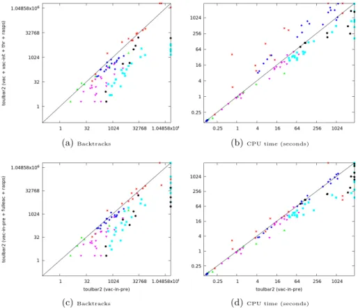
(a)Backtracks (b)CPU time (seconds)
(c)Backtracks (d)CPU time (seconds)
Fig. 2: Comparison with toulbar2 using VAC during search. CELAR: T, CPD:l, ProteinDesign:s, ProteinFolding:t, Warehouse:u, Worms:n.
(a)Backtracks (b)CPU time (seconds)
(c)Backtracks (d)CPU time (seconds)
Fig. 3: Comparison with default toulbar2. CELAR: T, CPD: l, ProteinDe-sign:s, ProteinFolding:t, Warehouse:u, Worms:n.
0 500 1000 1500 2000 2500 3000 3500 0 5 10 15 20 25 30
CPU time (in seconds)
Number of solved worms instances CombiLP (VAC+VAC-integral+threshold+RASPS)
CombiLP (VAC-in-preprocessing) toulbar2 (VAC-in-preprocessing+FullEAC+RASPS) toulbar2 (VAC+VAC-integral+threshold+RASPS) toulbar2 (VAC-in-preprocessing)
(a)Worms instances.
0 500 1000 1500 2000 2500 3000 3500 0 5 10 15 20
CPU time (in seconds)
Number of solved CPD instances toulbar2 (VAC-in-preprocessing+FullEAC+RASPS) CombiLP (VAC+VAC-integral+threshold+RASPS) CombiLP (VAC-in-preprocessing) toulbar2 (VAC+VAC-integral+threshold+RASPS) toulbar2 (VAC-in-preprocessing) (b)CPD instances.
Fig. 4: Comparison with CombiLP on Worms and CPD instances. value but it is not required to be unique in the domain. If a variable is kept, it means that its EAC value is fully compatible, i.e., has zero-cost, with all the
EAC values of its neighbors. We call it a Full EAC value. This approach can be combined with VAC-integrality. By restricting the EAC values to belong to the AC closure of Bool(P ) when the problem is made VAC, we ensure that any VAC-integral value is also Full EAC. The opposite is not true (see Supp. Fig. 1). Thus, the set of Full EAC values can be larger. We perform the Full EAC test in an incremental way (using a variable’s revise queue based on EAC value changes) at every node of the search tree, before choosing the next non Full EAC variable to branch on.
In order to improve this approach further, as soon as a new solution is found during search, EDAC will prefer to select the corresponding solution value as its EAC value for each unassigned variable if this value belongs to the current set of feasible EAC values. By doing so, we may exploit larger zero-cost partial assignments found previously during search. Notice that our branching heuristic is related to the min-conflicts repair algorithm [20] as it will only branch on variables in conflict with respect to a given assignment. Exploiting the best solution found so far for value heuristics has been shown to perform well on several constraint optimization problems when combined with restarts [10]. We use such a value ordering heuristic inside an hybrid best-first search algorithm [3] in all our experiments.
6
Relaxation-Aware Sub-Problem Search (RASPS)
One problem that branch-and-bound faces, especially in depth-first order, is that without a good upper bound it may explore large parts of the search tree that contain only poor quality solutions.
Here, we propose to use integrality information to try to quickly generate solutions that are close to the optimum. We describe a primal heuristic that we call Relaxation-Aware Sub-Problem Search (RASPS), which runs in preprocess-ing. We simply fix all VAC-integral variables to their values, prune values from the rest of the variables that are pruned in AC(Bool(P )), and then solve using the EDAC lower bound the resulting subproblem (see examples in Fig. 1d, 1f) to optimality or until a resource bound is met6. In order to choose the set of
VAC-integral variables, we use the dual solutions constructed in iterations of VAC before the last, hence examine Boolθ(P ) for an appropriate θ.
Although the idea of the heuristic is pretty straightforward, the key issue is to choose the threshold value (the θ) (recall Section 4) to construct Boolθ(P ),
as it has an impact on the quality of the upper bound produced and the time spent for this. To determine the threshold value for the RASPS, we observe the curves of the threshold θi, the ratio of VAC-integral variables ri, and the value
αi = ri/θi, collected during VAC iterations. The idea is that, once the ratio of
VAC-integral variables saturates, θi continues to decrease. As a result, αi starts
increasing more quickly which is the desired cutoff point. To identify that point,
6
In our implementation, we set an upper bound of 1000 backtracks for solving the subproblem.
we track of the curve of αiover the VAC iterations and choose the threshold value
when the angle of the curve reaches 10 degrees (see Supplementary Figure 2). This idea is related to the CombILP method of Haller et al. [13], described earlier. Compared to CombILP, RASPS solves a simpler combinatorial subprob-lem because of the larger VAC-integral set and the remaining pruned domains. Then, it only aims to produce a good initial upper bound and leaves proving optimality to the branch-and-bound solver.
Even more closely related is the RINS heuristic of Danna et al. [7]. It also searches for primal bounds by extending the integral part of the relaxation. In contrast to RASPS, it permits values of the incumbent solution and may be invoked in nodes other than the root. However, it has no way of distinguishing among integral variables as RASPS does with its choice of θ > 1. We have experimented with RASPS during search but have so far not found it worthwhile.
7
Experimental Results
We have implemented VAC-integrality and RASPS inside toulbar2, an open-source exact branch-and-bound WCSP solver in C++7. All computations were
performed on a single core of Intel Xeon E5-2680 v3 at 2.50 GHz and 256 GB of RAM with a 1-hour CPU time limit. No initial upper bounds were used, as is the default of the solver.
7.1 Benchmark description
We performed experiments on probabilistic and deterministic graphical models coming from different communities [15]. We considered a large set of 431 in-stances8which are all binary. It includes 251 instances (170 Auction, 16 CELAR,
10 ProteinDesign, 55 Warehouse) from the Cost Function Library9, 129 instances
(108 DBN, 21 ProteinFolding) from the Probabilistic Inference Challenge (PIC 2011)10
, 30 “Worms” instances [16] where CombiLP is state-of-the-art [13], and 21 Computational Protein Design (CPD) large instances for which toulbar2 is state-of-the-art [2,22]. We discarded Max-CSP, Max-SAT, Constraint Program-ming (CP), and Computer Vision (CVPR) instances which are either unweighted (all costs equal to 1), or non-binary, or being too easy (small search tree) or un-solved by all the tested approaches including MRF and ILP solvers [15].
7.2 Comparison with VAC
First, we compared our new heuristics with default VAC maintained during search (option -A=999999 for all tested methods). We skipped Auction and DBN as they do not have VAC-integral variables.
7
https://github.com/toulbar2/toulbar2, branch fural/strictac from version 1.0.1.
8 genoweb.toulouse.inra.fr/~degivry/evalgm 9 forgemia.inra.fr/thomas.schiex/cost-function-library 10 www.cs.huji.ac.il/project/PASCAL
In Fig. 2a, we show a scatter plot comparing the number of backtracks be-tween VAC and VAC exploiting VAC-integral variable heuristic. The size of the search tree is significantly reduced thanks to VAC-integrality for most instance families. Notice the logarithmic axes. The improvement in terms of CPU time (Fig. 2b) is less important but still significant for CPD, ProteinFolding, Worms, and some CELAR instances. However, we found several Warehouse instances where it was significantly slower using VAC-integrality. In this case, we found the explanation was a larger number of VAC iterations per search node (8 times more in average) corresponding to small lower bound improvements at small threshold values (θ near 1) that did not reduce the search tree sufficiently (only by a mean factor 2.2 on difficult Warehouse instances).
In order to avoid such pathological cases, we placed a bound on the minimum threshold value θ for VAC iterations during search. We selected the same limit as for RASPS (e.g., θ30 for Worms/cnd1threeL1 1228061). We found that using
this threshold mechanism alone speeds up Warehouse resolution and does not significantly deteriorate the results in the other families (see Supp. Fig. 4). Fur-thermore we obtained consistent results when combining with VAC-integrality, reducing the number of backtracks and CPU time for several families while being equivalent for the others (see Supp. Fig. 5).
Next, we analyzed the impact of applying the RASPS upper-bounding pro-cedure in preprocessing. We limit RASPS to 1000 backtracks. Again, our new heuristic RASPS significantly reduces the search effort in terms of backtracks and time, except for Warehouse and some CELAR. For Warehouse, the up-per bounds found did not reduce the total number of backtracks. For CELAR scen06 r, it reduces backtracks by 3.4 and solving time by 4.2. For Worms, it was more than 10 times faster for some instances (see Supp. Fig. 6).
Finally, we combine the two heuristics, VAC-integrality and RASPS, with VAC threshold limit and show the results compared to VAC alone in Fig. 2c and 2d. We keep this best configuration in the rest of the paper.
7.3 Comparison with VAC-in-preprocessing and CombiLP
One might expect using VAC only in preprocessing to be the fastest option, as it is the default for toulbar2 and significantly outperforms VAC during search in most cases [15]. For certain instance families, we manage to outperform it.
When VAC is used only in the preprocessing, using RASPS in addition con-siderably improves runtimes except for Warehouse and some CELAR (see Supp. Fig. 8). If we add VAC-integrality and RASPS when using VAC during search, we manage to outperform VAC in preprocessing for all families except CELAR and Warehouse, where the overhead of VAC is too high (see Fig. 3a and 3b).
Moreover, if we compare methods using VAC in preprocessing only, then exploiting our simpler Full EAC branching heuristic and RASPS performs even better in most cases, being as good as default toulbar2 on Warehouse instances (55 instances solved in average in 128 seconds) and comparable on CELAR (our approach solved graph13 and scen06 one-order-of-magnitude faster, but could not solve graph11 compared to default VAC in preprocessing, see Fig. 3c, 3d).
Next, we compare toulbar2 and CombiLP (which uses the same toulbar2 as its internal ILP solver) with different lower bound techniques, showing the advantages of exploiting VAC-integrality or Full EAC and RASPS extensions.
In Figure 4a, we see a cactus plot11 for the Worms benchmark where there are 30 instances. We solved these instances with different combinations of solvers and heuristics with a CPU time limit of 1 hour. CombiLP was reported to solve 25 of these instances in [13] within 1 hour CPU time. Here, we compare Com-biLP with parameters used in [13] (VAC in preprocessing and EDAC during search), as well as our version of toulbar2 plugged in it. In addition to those, we have standalone toulbar2 either with VAC in preprocessing and EDAC during search, with or without Full EAC, or VAC-integrality-aware branching, and RASPS options. toulbar2 alone can go up to 25 instances. However, by plugging our version of toulbar2 in CombiLP, we manage to solve 26 of these instances, which makes 1 more than [13]. Another important detail is that, al-though it is costly to use VAC throughout the search tree, it becomes better with VAC-integrality and RASPS. Still, it was slightly dominated by Full EAC. This simpler heuristic performed even better on the CPD benchmark (Fig. 4b). Our Full EAC heuristic with RASPS got the best results, solving 13 instances, compared to VAC-integrality and RASPS which solves 9, and only 8 by de-fault toulbar2. CombiLP using VAC during search with VAC-integrality and RASPS solved 11 instances, instead of 10 without these options and VAC in preprocessing.
8
Conclusions
We revisited the Strict Arc Consistency property which was recently used in an iterative relaxation solver. We identified properties that make it easier to use within a branch-and-bound solver and in particular in conjunction with the VAC algorithm. This property allows us to integrate information about the relaxation that VAC computes to be used in heuristics. We presented three new heuristics that exploit this information, two for branching and the other for finding good quality upper bounds. In an experimental evaluation, these heuristics showed great performance in some families of instances, improving on the previous state of the art. VAC-integrality identifies a single zero-cost satisfiable partial assignment in a particular CSP Bool(P ) of the original problem P . Other CSP techniques such as neighborhood substitutability [12] could be used to detect larger tractable sub-problems. The integral subproblem can also be viewed as a particularly easy tractable class, where each variable has a single value. Therefore, another possible direction is to detect subproblems that are tractable for more sophisticated reasons.
Acknowledgements This work has been partly funded by the “Agence na-tionale de la Recherche” (ANR-16-CE40-0028).
11
References
1. T Achterberg. Scip: solving constraint integer programs. Mathematical Program-ming Computation, 1(1):1–41, 2009.
2. D Allouche, J Davies, S de Givry, G Katsirelos, T Schiex, S Traor´e, I Andr´e, S Barbe, S Prestwich, and B O’Sullivan. Computational protein design as an optimization problem. Artificial Intelligence, 212:59–79, 2014.
3. D Allouche, S de Givry, G Katsirelos, T Schiex, and M Zytnicki. Anytime Hybrid Best-First Search with Tree Decomposition for Weighted CSP. In Proc. of CP-15, pages 12–28, Cork, Ireland, 2015.
4. F Bacchus, X Chen, P van Beek, and T Walsh. Binary vs. non-binary constraints. Artificial Intelligence, 140(1/2):1–37, 2002.
5. F Boussemart, F Hemery, C Lecoutre, and L Sais. Boosting systematic search by weighting constraints. In Proc. of ECAI-04, pages 146–150, Valencia, Spain, 2004. 6. M Cooper, S De Givry, M S´anchez, T Schiex, M Zytnicki, and T Werner. Soft arc
consistency revisited. Artificial Intelligence, 174(7-8):449–478, 2010.
7. E Danna, E Rothberg, and C Le Pape. Exploring relaxation induced neighborhoods to improve mip solutions. Mathematical Programming, 102(1):71–90, 2005. 8. J Davies and F Bacchus. Solving maxsat by solving a sequence of simpler sat
instances. In Proc. of CP-11, pages 225–239, Perugia, Italy, 2011.
9. S de Givry, M Zytnicki, F Heras, and J Larrosa. Existential arc consistency: getting closer to full arc consistency in weighted CSPs. In Proc. of IJCAI-05, pages 84–89, Edinburgh, Scotland, 2005.
10. Emir Demirovic, Geoffrey Chu, and Peter J. Stuckey. Solution-based phase saving for CP: A value-selection heuristic to simulate local search behavior in complete solvers. In Proc. of CP-18, pages 99–108, Lille, France, 2018.
11. R G. Downey and M R. Fellows. Fundamentals of Parameterized Complexity. Texts in Computer Science. Springer, 2013.
12. E C. Freuder. Eliminating interchangeable values in constraint satisfaction prob-lems. In Proc. of AAAI’91, pages 227–233, Anaheim, CA, 1991.
13. S Haller, P Swoboda, and B Savchynskyy. Exact map-inference by confining com-binatorial search with LP relaxation. In Proc. of AAAI-18, pages 6581–6588, New Orleans, Louisiana, USA, 2018.
14. F. Heras and J. Larrosa. New Inference Rules for Efficient Max-SAT Solving. In Proc. of the National Conference on Artificial Intelligence, AAAI-2006, 2006. 15. B Hurley, B O’Sullivan, D Allouche, G Katsirelos, T Schiex, M Zytnicki, and
S de Givry. Multi-Language Evaluation of Exact Solvers in Graphical Model Dis-crete Optimization. Constraints, 21(3):413–434, 2016.
16. D Kainmueller, F Jug, C Rother, and G Myers. Active graph matching for auto-matic joint segmentation and annotation of c. elegans. In Medical Image Computing and Computer-Assisted Intervention, pages 81–88, Boston, USA, 2014.
17. D Koller and N Friedman. Probabilistic graphical models: principles and techniques. The MIT Press, 2009.
18. V Kolmogorov. Convergent tree-reweighted message passing for energy minimiza-tion. IEEE transactions on pattern analysis and machine intelligence, 28(10):1568– 1583, 2006.
19. C Lecoutre, L Sais, S Tabary, and V Vidal. Reasoning from last conflict(s) in constraint programming. Artificial Intelligence, 173(18):1592–1614, 2009.
20. S Minton, M Johnston, A Philips, and P Laird. Minimizing conflicts: a heuris-tic repair method for constraint satisfaction and scheduling problems. Artificial Intelligence, 58:160–205, 1992.
21. A Morgado, A Ignatiev, and J Marques-Silva. MSCG: robust core-guided maxsat solving. JSAT, 9:129–134, 2014.
22. A Ouali, D Allouche, S de Givry, S Loudni, Y Lebbah, L Loukil, and P Boizumault. Variable neighborhood search for graphical model energy minimization. Artificial Intelligence, 278(103194):22p., 2020.
23. B Savchynskyy, JH Kappes, P Swoboda, and C Schn¨orr. Global map-optimality by shrinking the combinatorial search area with convex relaxation. In Proc. of NIPS-13, pages 1950–1958, Lake Tahoe, Nevada, USA, 2013.
24. D Sontag, T Meltzer, A Globerson, Y Weiss, and T Jaakkola. Tightening LP relax-ations for MAP using message-passing. In Proc. of UAI, pages 503–510, Helsinki, Finland, 2008.