Research Article
Andrea Marchese and Annalisa Massaccesi
The Steiner tree problem revisited through
rectifiable 𝐺-currents
Abstract: The Steiner tree problem can be stated in terms of finding a connected set of minimal length containing a given set of finitely many points. We show how to formulate it as a mass-minimization problem for 1-dimensional currents with coefficients in a suitable normed group. The representation used for these currents allows to state a calibration principle for this problem. We also exhibit calibrations in some examples.
Keywords: Steiner tree problem, rectifiable currents, calibration, flat 𝐺-chains MSC 2010: 49Q15, 49Q20
||
Andrea Marchese: Max-Planck-Institut für Mathematik in den Naturwissenschaften, Inselstraße 22, 04103 Leipzig, Germany,
e-mail: [email protected]
Annalisa Massaccesi: Institut für Mathematik der Universität Zürich, Winterthurerstrasse 190, CH-8057 Zürich, Switzerland,
e-mail: [email protected]
Communicated by: Giuseppe Mingione
Introduction
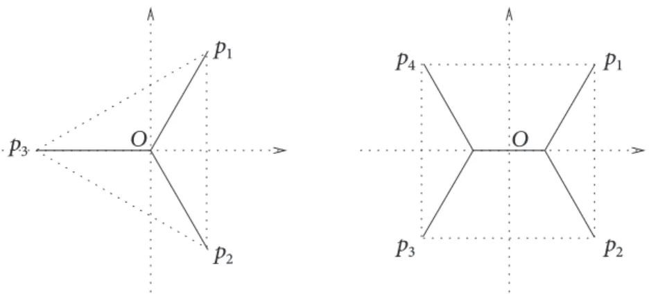
The classical Steiner tree problem consists in finding the shortest connected set containing 𝑛 given distinct points 𝑝1, . . . , 𝑝𝑛in ℝ𝑑. Some very well-known examples are shown in Figure 1.
DOI 10.1515/acv-2014-0022 | Adv. Calc. Var. 2014; ??? (???):1–22
Research Article
Andrea Marchese and Annalisa Massaccesi
The Steiner tree problem revisited through
rectifiable 𝐺-currents
Abstract: The Steiner tree problem can be stated in terms of finding a connected set of minimal length
containing a given set of finitely many points. We show how to formulate it as a mass-minimization problem for 1-dimensional currents with coefficients in a suitable normed group. The representation used for these currents allows to state a calibration principle for this problem. We also exhibit calibrations in some examples.
Keywords: Steiner tree problem, rectifiable currents, calibration, flat 𝐺-chains MSC 2010: 49Q15, 49Q20
||
Andrea Marchese: Max-Planck-Institut für Mathematik in den Naturwissenschaften, Inselstraße 22, 04103 Leipzig, Germany,
e-mail: [email protected]
Annalisa Massaccesi: Institut für Mathematik der Universität Zürich, Winterthurerstrasse 190, CH-8057 Zürich, Switzerland,
e-mail: [email protected]
Communicated by: Guiseppe Mingione
Introduction
The classical Steiner tree problem consists in finding the shortest connected set containing 𝑛 given distinct points 𝑝1, . . . , 𝑝𝑛in ℝ𝑑. Some very well-known examples are shown in Figure 1.
𝑝
4𝑝
3𝑝
1𝑝
2𝑂
𝑝
1𝑝
2𝑝
3𝑂
Figure 1. Solutions for the vertices of an equilateral triangle and a square.
The problem is completely solved in ℝ2and there exists a wide literature on the subject, mainly devoted
to improving the efficiency of algorithms for the construction of solutions: see, for instance, [13] and [14] for a survey of the problem. The recent papers [22] and [23] witness the current studies on the problem and its generalizations.
Our aim is to rephrase the Steiner tree problem as an equivalent mass-minimization problem by replacing connected sets with 1-currents with coefficients in a more suitable group than ℤ, in such a way that solutions
Figure 1. Solutions for the vertices of an equilateral triangle and a square.
The problem is completely solved in ℝ2and there exists a wide literature on the subject, mainly devoted
to improving the efficiency of algorithms for the construction of solutions: see, for instance, [13] and [14] for a survey of the problem. The recent papers [22] and [23] witness the current studies on the problem and its generalizations.
Our aim is to rephrase the Steiner tree problem as an equivalent mass-minimization problem by replacing connected sets with 1-currents with coefficients in a more suitable group than ℤ, in such a way that solutions of one problem correspond to solutions of the other, and vice-versa. The use of currents allows to exploit techniques and tools from the Calculus of Variations and the Geometric Measure Theory.
20 | A. Marchese and A. Massaccesi, The Steiner tree problem revisited
2 | A. Marchese and A. Massaccesi, The Steiner tree problem revisited
of one problem correspond to solutions of the other, and vice-versa. The use of currents allows to exploit techniques and tools from the Calculus of Variations and the Geometric Measure Theory.
Let us briefly point out a few facts suggesting that classical polyhedral chains with integer coefficients might not be the correct environment for our problem. First of all, one should make the given points 𝑝1, . . . , 𝑝𝑛
in the Steiner problem correspond to some integral polyhedral 0-chain supported on 𝑝1, . . . , 𝑝𝑛, with suitable
multiplicities 𝑚1, . . . , 𝑚𝑛. One has to impose that 𝑚1+ ⋅ ⋅ ⋅ + 𝑚𝑛= 0 in order that this 0-chain is the boundary
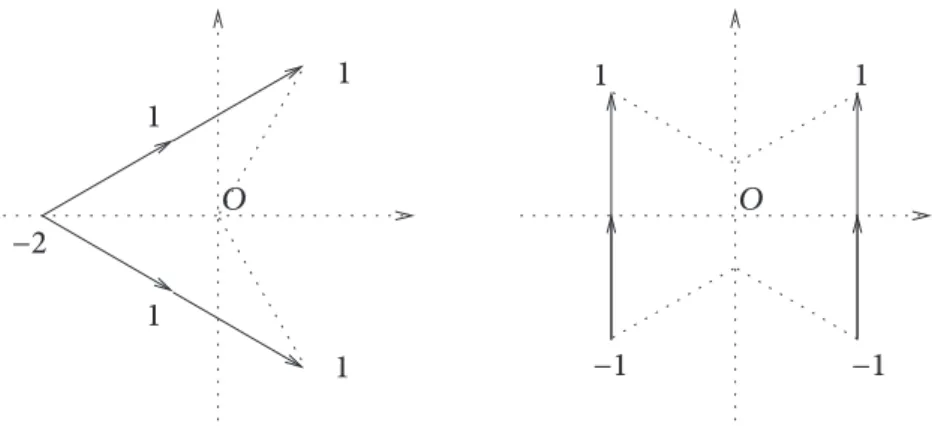
of a compactly supported 1-chain. In the example of the equilateral triangle, see Figure 1, the condition 𝑚3= −(𝑚1+ 𝑚2) forces to break symmetry, leading to the minimizer in Figure 2. The desired solution is
instead depicted in Figure 1. In the second example from Figure 1, we get the “wrong” non-connected minimizer even though all boundary multiplicities have modulus 1; see Figure 2.
𝑂
𝑂
1
1
1
−1
−1
1
1
−2
1
Figure 2. Solutions for the mass-minimization problems among polyhedral chains with integer coefficients.
These examples show that ℤ is not the right group of coefficients.
Our framework will be that of currents with coefficients in a normed abelian group 𝐺 (briefly: 𝐺-currents), which we will introduce in Section 1.
Currents with coefficients in a group were introduced by W. Fleming. There is a vast literature on the subject: let us mention only the seminal paper [12], the work of B. White [26, 27], and the more recent papers by T. De Pauw and R. Hardt [8] and by L. Ambrosio and M. G. Katz [3]. A closure theorem holds for these flat 𝐺-chains, see [12] and [26].
In Section 2 we recast the Steiner problem in terms of a mass-minimization problem over currents with coefficients in a discrete group 𝐺, chosen only on the basis of the number of boundary points. As we already said, this construction provides a way to pass from a mass-minimizer to a Steiner solution and vice-versa.
This new formulation permits to initiate a study of calibrations as a sufficient condition for minimality; this is the subject of Section 3. Classically a calibration 𝜔 associated with a given oriented 𝑘-submanifold 𝑆 ⊂ ℝ𝑑is a unit closed 𝑘-form taking value 1 on the tangent space of 𝑆. The existence of a calibration
guaran-tees the minimality of 𝑆 among oriented submanifolds with the same boundary 𝜕𝑆. Indeed, Stokes’ theorem and the assumptions on 𝜔 imply that
vol(𝑆) = ∫
𝑆
𝜔 = ∫
𝑆
𝜔 ≤ vol(𝑆),
for any submanifold 𝑆having the same boundary of 𝑆.
In order to define calibrations in the framework of 𝐺-currents, it is convenient to view currents as linear functionals on forms, which is not always possible in the usual setting of currents with coefficients in groups. This motivates the preliminary work in Section 1, where we embed the group 𝐺 in a normed linear space 𝐸 and we construct the currents with coefficients in 𝐸 in the classical way. In Definition 3.5, the notion of calibration is slightly weakened in order to include piecewise smooth forms, which appear in
Figure 2. Solutions for the mass-minimization problems among polyhedral chains with integer coefficients.
Let us briefly point out a few facts suggesting that classical polyhedral chains with integer coefficients might not be the correct environment for our problem. First of all, one should make the given points 𝑝1, . . . , 𝑝𝑛
in the Steiner problem correspond to some integral polyhedral 0-chain supported on 𝑝1, . . . , 𝑝𝑛, with suitable
multiplicities 𝑚1, . . . , 𝑚𝑛. One has to impose that 𝑚1+ ⋅ ⋅ ⋅ + 𝑚𝑛= 0 in order that this 0-chain is the boundary
of a compactly supported 1-chain. In the example of the equilateral triangle, see Figure 1, the condition 𝑚3= −(𝑚1+ 𝑚2) forces to break symmetry, leading to the minimizer in Figure 2. The desired solution is instead depicted in Figure 1. In the second example from Figure 1, we get the “wrong” non-connected minimizer even though all boundary multiplicities have modulus 1; see Figure 2.
These examples show that ℤ is not the right group of coefficients.
Our framework will be that of currents with coefficients in a normed abelian group 𝐺 (briefly: 𝐺-currents), which we will introduce in Section 1.
Currents with coefficients in a group were introduced by W. Fleming. There is a vast literature on the subject: let us mention only the seminal paper [12], the work of B. White [26, 27], and the more recent papers by T. De Pauw and R. Hardt [8] and by L. Ambrosio and M. G. Katz [3]. A closure theorem holds for these flat 𝐺-chains, see [12] and [26].
In Section 2 we recast the Steiner problem in terms of a mass-minimization problem over currents with coefficients in a discrete group 𝐺, chosen only on the basis of the number of boundary points. As we already said, this construction provides a way to pass from a mass-minimizer to a Steiner solution and vice-versa.
This new formulation permits to initiate a study of calibrations as a sufficient condition for minimality; this is the subject of Section 3. Classically a calibration 𝜔 associated with a given oriented 𝑘-submanifold 𝑆 ⊂ ℝ𝑑is a unit closed 𝑘-form taking value 1 on the tangent space of 𝑆. The existence of a calibration
guaran-tees the minimality of 𝑆 among oriented submanifolds with the same boundary 𝜕𝑆. Indeed, Stokes’ theorem and the assumptions on 𝜔 imply that
vol(𝑆) = ∫
𝑆
𝜔 = ∫
𝑆
𝜔 ≤ vol(𝑆), for any submanifold 𝑆having the same boundary of 𝑆.
In order to define calibrations in the framework of 𝐺-currents, it is convenient to view currents as linear functionals on forms, which is not always possible in the usual setting of currents with coefficients in groups. This motivates the preliminary work in Section 1, where we embed the group 𝐺 in a normed linear space 𝐸 and we construct the currents with coefficients in 𝐸 in the classical way. In Definition 3.5, the notion of calibration is slightly weakened in order to include piecewise smooth forms, which appear in Examples 3.10 and 3.11, where we exhibit calibrations for the problem on the right of Figure 1 and for the Steiner tree problem on the vertices of a regular hexagon plus the center. It is worthwhile to note that our theory works for the Steiner tree problem in ℝ𝑑and for currents supported in ℝ𝑑; we made explicit
computa-tions only on 2-dimensional configuracomputa-tions for simplicity reasons. We conclude Section 3 with some remarks concerning the use of calibrations in similar contexts, see for instance [19].
The existence of a calibration is a sufficient condition for a manifold to be a minimizer; one could wonder whether this condition is necessary as well. In general, a smooth (or piecewise smooth, according to Definition 3.7) calibration might not exist; nevertheless, one can still search for some weak calibration, for instance a differential form with bounded measurable coefficients. In Section 4 we discuss a strategy in order to get the existence of such a weak calibration. A duality argument due to H. Federer [11] ensures that a weak calibration exists for mass-minimizing normal currents; the same argument works for mass-minimizing normal currents with coefficients in the normed vector space 𝐸. Therefore an equivalence principle between minima among normal and rectifiable 1-currents with coefficients in 𝐸 and 𝐺, respectively, is sufficient to conclude that a calibration exists. Proposition 4.3 guarantees that the equivalence between minima holds in the case of classical 1-currents with real coefficients; hence a weak calibration always exists. The proof of this result is subject to the validity of a homogeneity property for the candidate minimizer stated in Remark 4.4. Example 4.5 shows that for 1-dimensional 𝐺-currents an interesting new phenomenon occurs, since (at least in a non-Euclidean setting) this homogeneity property might not hold; the validity of the homogeneity prop-erty may be related to the ambient space. The problem of the existence of a calibration in the Euclidean space is still open.
1 Rectifiable currents over a coefficient group
In this section we provide definitions for currents over a coefficient group, with some basic examples. Fix an open set 𝑈 ⊂ ℝ𝑑and a normed vector space (𝐸, ‖ ⋅ ‖
𝐸) with finite dimension 𝑚 ≥ 1. We will denote
by (𝐸∗, ‖ ⋅ ‖
𝐸∗) its dual space endowed with the dual norm
‖𝑓‖𝐸∗:= sup
‖𝑣‖𝐸≤1
⟨𝑓; 𝑣⟩. Definition 1.1. We say that a map
𝜔 : Λ𝑘(ℝ𝑑) × 𝐸 → ℝ
is an 𝐸∗-valued 𝑘-covector in ℝ𝑑if
(i) for all 𝜏 ∈ Λ𝑘(ℝ𝑑), 𝜔(𝜏, ⋅ ) ∈ 𝐸∗, that is, 𝜔(𝜏, ⋅ ) : 𝐸 → ℝ is a linear function.
(ii) for all 𝑣 ∈ 𝐸, 𝜔( ⋅ , 𝑣) : Λ𝑘(ℝ𝑑) → ℝ is a (classical) 𝑘-covector.
Sometimes we will use ⟨𝜔; 𝜏, 𝑣⟩ instead of 𝜔(𝜏, 𝑣), in order to simplify the notation. The space of 𝐸∗-valued
𝑘-covectors in ℝ𝑑is denoted by Λ𝑘
𝐸(ℝ𝑑) and it is endowed with the comass norm
‖𝜔‖ := sup{‖𝜔(𝜏, ⋅ )‖𝐸∗: |𝜏| ≤ 1, 𝜏 simple}. (1.1)
Remark 1.2. Fix an orthonormal system of coordinates in ℝ𝑑, (e
1, . . . , e𝑑); the corresponding dual base
in (ℝ𝑑)∗is (𝑑𝑥
1, . . . , 𝑑𝑥𝑑). Consider a complete biorthonormal system for 𝐸, i.e. a pair
(𝑣1, . . . , 𝑣𝑚) ∈ 𝐸𝑚, (𝑤1, . . . , 𝑤𝑚) ⊂ (𝐸∗)𝑚
such that ‖𝑣𝑖‖𝐸= 1, ‖𝑤𝑖‖𝐸∗ = 1 and ⟨𝑤𝑖; 𝑣𝑗⟩ = 𝛿𝑖𝑗. Given an 𝐸∗-valued 𝑘-covector 𝜔, we denote
𝜔𝑗:= 𝜔( ⋅ , 𝑣 𝑗).
For each 𝑗 ∈ {1, . . . , 𝑚}, 𝜔𝑗 is a 𝑘-covector in the usual sense. Hence the biorthonormal system (𝑣
1, . . . , 𝑣𝑚),
(𝑤1, . . . , 𝑤𝑚) allows to write 𝜔 in “components”
𝜔 = (𝜔1, . . . , 𝜔𝑚), in fact we have 𝜔(𝜏, 𝑣) =∑𝑚 𝑗=1⟨𝜔 𝑗; 𝜏⟩⟨𝑤 𝑗; 𝑣⟩.
In particular 𝜔𝑗admits the usual representation
𝜔𝑗 = ∑
1≤𝑖1<⋅⋅⋅<𝑖𝑘≤𝑑
22 | A. Marchese and A. Massaccesi, The Steiner tree problem revisited
Definition 1.3. An 𝐸∗-valued differential 𝑘-form in 𝑈 ⊂ ℝ𝑑, or just a 𝑘-form when it is clear which vector space
we are referring to, is a map
𝜔 : 𝑈 → Λ𝑘𝐸(ℝ𝑑);
we say that 𝜔 isC∞-regular if every component 𝜔𝑗is so (see Remark 1.2). We denote byC𝑐∞(𝑈, Λ𝑘𝐸(ℝ𝑑)) the
vector space ofC∞-regular 𝐸∗-valued 𝑘-forms with compact support in 𝑈.
We are mainly interested in 𝐸∗-valued 1-forms, nevertheless we analyze 𝑘-forms in wider generality, in order
to ease other definitions, such as the differential of an 𝐸∗-valued form and the boundary of an 𝐸-current. Definition 1.4. We define the differential d𝜔 of aC∞-regular 𝐸∗-valued 𝑘-form 𝜔 by components:
d𝜔𝑗:= d(𝜔𝑗) : 𝑈 → Λ𝑘+1(ℝ𝑑), 𝑗 = 1, . . . , 𝑚,
Moreover,C𝑐∞(𝑈, Λ1𝐸(ℝ𝑑)) has a norm, denoted by ‖ ⋅ ‖, given by the supremum of the comass norm of the
form defined in (1.1). Hence we mean
‖𝜔‖ := sup
𝑥∈𝑈‖𝜔(𝑥)‖. (1.2)
Definition 1.5. A 𝑘-dimensional current 𝑇 in 𝑈 ⊂ ℝ𝑑, with coefficients in 𝐸, or just an 𝐸-current when there is
no doubt on the dimension, is a linear and continuous function 𝑇 :C𝑐∞(𝑈, Λ𝑘𝐸(ℝ𝑑)) → ℝ,
where the continuity is meant with respect to the locally convex topology on the space C𝑐∞(𝑈, Λ𝑘𝐸(ℝ𝑑)),
built in analogy with the topology onC𝑐∞(ℝ𝑛), with respect to which distributions are dual. This defines the
weak∗topology on the space of 𝑘-dimensional 𝐸-currents. Convergence in this topology is equivalent to the
convergence of all the “components” in the space of classical¹ 𝑘-currents, by which we mean the following. We define for every 𝑘-dimensional 𝐸-current 𝑇 its components 𝑇𝑗, for 𝑗 = 1, . . . , 𝑚, and we write
𝑇 = (𝑇1, . . . , 𝑇𝑚), denoting
⟨𝑇𝑗; 𝜑⟩ := ⟨𝑇; ̃𝜑𝑗⟩,
for every (classical) compactly supported differential 𝑘-form 𝜑 on ℝ𝑑. Here ̃𝜑
𝑗denotes the 𝐸∗-valued
differen-tial 𝑘-form on ℝ𝑑such that
̃𝜑𝑗( ⋅ , 𝑣𝑗) = 𝜑, (1.3)
̃𝜑𝑗( ⋅ , 𝑣𝑖) = 0 for 𝑖 ̸= 𝑗. (1.4)
It turns out that a sequence of 𝑘-dimensional 𝐸-currents 𝑇ℎweakly∗converges to an 𝐸-current 𝑇 (in this case
we write 𝑇ℎ⇀ 𝑇) if and only if the sequence of the components 𝑇∗ ℎ𝑗 converge to 𝑇𝑗 in the space of classical
𝑘-currents, for 𝑗 = 1, . . . , 𝑚.
Definition 1.6. For a 𝑘-current 𝑇 over 𝐸 we define the boundary operator
⟨𝜕𝑇; 𝜑⟩ := ⟨𝑇; d𝜑⟩ for all 𝜑 = (𝜑1, . . . , 𝜑𝑚) ∈C𝑐∞(𝑈, Λ𝑘−1𝐸 (ℝ𝑑))
and the mass
𝕄(𝑇) := sup
‖𝜔‖≤1⟨𝑇; 𝜔⟩.
As one can expect, the boundary 𝜕(𝑇𝑗) of every component 𝑇𝑗 is the relative component (𝜕𝑇)𝑗of the
boundary 𝜕𝑇.
Definition 1.7. A 𝑘-dimensional normal 𝐸-current in 𝑈 ⊂ ℝ𝑑is an 𝐸-current 𝑇 with the properties 𝕄(𝑇) < +∞
and 𝕄(𝜕𝑇) < +∞. Thanks to the Riesz Theorem, 𝑇 admits the following representation: ⟨𝑇; 𝜔⟩ = ∫
𝑈
⟨𝜔(𝑥); 𝜏(𝑥), 𝑣(𝑥)⟩ d𝜇𝑇(𝑥) for all 𝜔 ∈C𝑐∞(𝑈, Λ𝑘𝐸(ℝ𝑑)),
where 𝜇𝑇is a Radon measure on 𝑈, 𝑣 : 𝑈 → 𝐸 is summable with respect to 𝜇𝑇and |𝜏| = 1, 𝜇𝑇-a.e. A similar
representation holds for the boundary 𝜕𝑇.
Definition 1.8. A rectifiable 𝑘-current 𝑇 in 𝑈 ⊂ ℝ𝑑, over 𝐸, or a rectifiable 𝐸-current is an 𝐸-current admitting
the following representation: ⟨𝑇; 𝜔⟩ := ∫
Σ
⟨𝜔(𝑥); 𝜏(𝑥), 𝜃(𝑥)⟩ dH𝑘(𝑥) for all 𝜔 ∈C𝑐∞(ℝ𝑑, Λ𝑘𝐸(𝑈))
where Σ is a countably 𝑘-rectifiable set (see [16, Definition 5.4.1]) contained in 𝑈, 𝜏(𝑥) ∈ 𝑇𝑥Σ with |𝜏(𝑥)| = 1
forH𝑘-a.e. 𝑥 ∈ Σ and 𝜃 ∈ 𝐿1(H𝑘 Σ; 𝐸). We will refer to such a current as 𝑇 = 𝑇(Σ, 𝜏, 𝜃). If 𝐵 is a Borel set and
𝑇(Σ, 𝜏, 𝜃) is a rectifiable 𝐸-current, we denote by 𝑇 𝐵 the current 𝑇(Σ ∩ 𝐵, 𝜏, 𝜃).
Consider now a discrete subgroup 𝐺 < 𝐸, endowed with the restriction of the norm ‖ ⋅ ‖𝐸. If the multiplicity 𝜃
takes only values in 𝐺, and if the same holds in the representation of 𝜕𝑇, we call 𝑇 a rectifiable 𝐺-current. Pay attention to the fact that, in the framework of currents over the coefficient group 𝐸, rectifiable 𝐸-currents play the role of (classical) rectifiable current, while rectifiable 𝐺-currents correspond to (classical) integral currents. Actually this correspondence is an equality, when 𝐸 is the group ℝ (with the Euclidean norm) and 𝐺 is ℤ.
The next proposition gives a formula to compute the mass of a 1-dimensional rectifiable 𝐸-current. Proposition 1.9. Let 𝑇 = 𝑇(Σ, 𝜏, 𝜃) be a 1-dimensional rectifiable 𝐸-current. Then
𝕄(𝑇) = ∫
Σ
‖𝜃(𝑥)‖𝐸dH1(𝑥).
Since the mass is lower semicontinuous, we can apply the direct method of the Calculus of Variations for the existence of minimizers with given boundary, once we provide the following compactness result. Here we assume for simplicity that 𝐺 is the subgroup of 𝐸 generated by 𝑣1, . . . , 𝑣𝑚(see Remark 1.2). A similar argument
works for every discrete subgroup 𝐺.
Theorem 1.10. Let (𝑇ℎ)ℎ≥1be a sequence of rectifiable 𝐺-currents such that there exists a positive finite
con-stant 𝐶 satisfying
𝕄(𝑇ℎ) + 𝕄(𝜕𝑇ℎ) ≤ 𝐶 for every ℎ ≥ 1.
Then there exists a subsequence (𝑇ℎ𝑖)𝑖≥1and a rectifiable 𝐺-current 𝑇 such that
𝑇ℎ𝑖
∗
⇀ 𝑇.
Proof. The statement of the theorem can be proved component by component. In fact, let 𝑇1
ℎ, . . . , 𝑇ℎ𝑚be the
components of 𝑇ℎ. Since (𝑣1, . . . , 𝑣𝑚), (𝑤1, . . . , 𝑤𝑚) is a biorthonormal system, we have
𝕄(𝑇ℎ𝑗) + 𝕄(𝜕𝑇ℎ𝑗) ≤ 𝑚(𝕄(𝑇ℎ) + 𝕄(𝜕𝑇ℎ)) ≤ 𝑚𝐶,
hence, after a diagonal procedure, we can find a subsequence (𝑇ℎ𝑖)𝑖≥1such that (𝑇
𝑗
ℎ𝑖)𝑖≥1weakly
∗converges to
some integral current 𝑇𝑗, for every 𝑗 = 1, . . . , 𝑚. Denoting by 𝑇 the rectifiable 𝐺-current, whose components
are 𝑇1, . . . , 𝑇𝑚, we have
𝑇ℎ𝑖
∗
⇀ 𝑇.
We conclude this section with some notations and basic facts about certain classes of rectifiable 𝐸-currents. Given a Lipschitz path 𝛾 : [0, 1] → ℝ2(parameterized with constant speed), and a coefficient 𝑔 ∈ 𝐺, we define
24 | A. Marchese and A. Massaccesi, The Steiner tree problem revisited
by ℓ(Γ) the length of the curve Γ, the orientation 𝜏 is defined by 𝜏(𝛾(𝑡)) := 𝛾(𝑡)/ℓ(Γ) for a.e. 𝑡 ∈ [0, 1]. It turns
out that the boundary of such a current is 𝜕𝑇 = 𝑔𝛿𝛾(1)− 𝑔𝛿𝛾(0), where the notation means that for every smooth
𝐸∗-valued map 𝜔, there holds
⟨𝜕𝑇; 𝜔⟩ = ⟨𝜔(𝛾(1)); 𝑔⟩ − ⟨𝜔(𝛾(0)); 𝑔⟩.
Using this notation, we observe that, given some points 𝑃1, . . . , 𝑃𝑘 and some multiplicities 𝑔1, . . . , 𝑔𝑘in 𝐺,
the 0-dimensional rectifiable 𝐺-current 𝑆 = 𝑔1𝛿𝑃1+ ⋅ ⋅ ⋅ + 𝑔𝑘𝛿𝑃𝑘is the boundary of some 1-dimensional
rectifi-able 𝐺-current with compact support 𝑇 if and only if 𝑔1+ ⋅ ⋅ ⋅ + 𝑔𝑘= 0.
2 Steiner tree problem revisited
In this section we establish the equivalence between the Steiner tree problem and a mass-minimization problem in a family of 𝐺-currents. We firstly need to choose the right group of coefficients 𝐺. Once we fix the number 𝑛 of points in the Steiner problem, we construct a normed vector space (𝐸, ‖ ⋅ ‖𝐸) and a subgroup 𝐺
of 𝐸, satisfying the following properties:
(P1) There exist 𝑔1, . . . , 𝑔𝑛−1 ∈ 𝐺 and ℎ1, . . . , ℎ𝑛−1∈ 𝐸∗such that (𝑔1, . . . , 𝑔𝑛−1) with (ℎ1, . . . , ℎ𝑛−1) is a complete
biorthonormal system for 𝐸 and 𝐺 is generated by 𝑔1, . . . , 𝑔𝑛−1.
(P2) ‖𝑔𝑖1+ ⋅ ⋅ ⋅ + 𝑔𝑖𝑘‖𝐸= 1 whenever 1 ≤ 𝑖1< ⋅ ⋅ ⋅ < 𝑖𝑘≤ 𝑛 − 1 and 𝑘 ≤ 𝑛 − 1.
(P3) ‖𝑔‖𝐸≥ 1 for every 𝑔 ∈ 𝐺 \ {0}.
(P4) Let 𝜃 = ∑𝑛−1
𝑗=1𝜃𝑗𝑔𝑗and ̃𝜃 = ∑𝑛−1𝑗=1 ̃𝜃𝑗𝑔𝑗satisfy the following condition:
{ { { 0 ≤ ̃𝜃𝑗≤ 𝜃𝑗 when 𝜃𝑗 ≥ 0, 0 ≥ ̃𝜃𝑗≥ 𝜃𝑗 otherwise. Then ‖̃𝜃‖𝐸≤ ‖𝜃‖𝐸.
For the moment we will assume the existence of 𝐺 and 𝐸. The proof of their existence and an explicit repre-sentation, useful for the computations, are given in Lemma 2.6.
The next lemma has a fundamental role: through it, we can give a nice structure of 1-dimensional recti-fiable 𝐺-current to every suitable competitor for the Steiner tree problem. From now on we will denote
𝑔𝑛:= −(𝑔1+ ⋅ ⋅ ⋅ + 𝑔𝑛−1).
Lemma 2.1. Let 𝐵 be a compact and connected set with finite length in ℝ𝑑, containing the points 𝑝
1, . . . , 𝑝𝑛.
Then there exists a connected set 𝐵⊂ 𝐵 containing 𝑝
1, . . . , 𝑝𝑛 and a 1-dimensional rectifiable 𝐺-current
𝑇𝐵 = 𝑇(𝐵, 𝜏, 𝜃) such that
(i) ‖𝜃(𝑥)‖𝐸= 1 for a.e. 𝑥 ∈ 𝐵,
(ii) 𝜕𝑇𝐵is the 0-dimensional 𝐺-current 𝑔1𝛿𝑝
1+ ⋅ ⋅ ⋅ + 𝑔𝑛𝛿𝑝𝑛.
Proof. Since 𝐵 is a connected, compact set of finite length, it follows that 𝐵 is connected by paths of finite length (see [9, Lemma 3.12]). Consider a curve 𝐵1which is the image of an injective path contained in 𝐵 going
from 𝑝1to 𝑝𝑛and associate to it the rectifiable 𝐺-current 𝑇1with multiplicity −𝑔1, as explained in Section 1.
Repeat this procedure keeping the end-point 𝑝𝑛and replacing at each step 𝑝1with 𝑝2, . . . , 𝑝𝑛−1. To be precise,
in this procedure, as soon as a curve 𝐵𝑖intersects another curve 𝐵𝑗with 𝑗 < 𝑖, we force 𝐵𝑖to coincide with 𝐵𝑗
from that intersection point to the end-point 𝑝𝑛. The set 𝐵= 𝐵1∪ ⋅ ⋅ ⋅ ∪ 𝐵𝑛−1 ⊂ 𝐵 is a connected set containing
the points 𝑝1, . . . , 𝑝𝑛and the 1-dimensional rectifiable 𝐺-current 𝑇 = 𝑇1+ ⋅ ⋅ ⋅ + 𝑇𝑛−1satisfies the requirements
of the lemma, in particular condition (i) is a consequence of (P2).
Via the next lemma (Lemma 2.3), we can say that solutions to the mass-minimization problem defined in Theorem 2.4 have connected supports. For the proof we need the following theorem on the structure of classical integral 1-currents. This theorem has firstly been stated as a corollary of [10, Theorem 4.2.25]. It allows us to consider an integral 1-current as a countable sum of oriented simple Lipschitz curves with integer multiplicities.
Theorem 2.2. Let 𝑇 be an integral 1-current in ℝ𝑑. Then 𝑇 =∑𝐾 𝑘=1𝑇𝑘+ ∞ ∑ ℓ=1𝐶ℓ (2.1) with
(i) 𝑇𝑘are integral 1-currents associated to injective Lipschitz paths for every 𝑘 = 1, . . . , 𝐾, and 𝐶ℓare integral
1-currents associated to Lipschitz paths which have the same value at 0 and 1 and are injective on (0, 1) for every ℓ ≥ 1,
(ii) 𝜕𝐶ℓ= 0 for every ℓ ≥ 1.
Moreover 𝕄(𝑇) =∑𝐾 𝑘=1 𝕄(𝑇𝑘) +∑∞ ℓ=1 𝕄(𝐶ℓ) (2.2) and 𝕄(𝜕𝑇) =∑𝐾 𝑘=1 𝕄(𝜕𝑇𝑘). (2.3)
Lemma 2.3. Let 𝑇 = 𝑇(Σ, 𝜏, 𝜃) be a 1-dimensional rectifiable 𝐺-current such that the boundary 𝜕𝑇 is the 0-current 𝑔1𝛿𝑝1+ ⋅ ⋅ ⋅ + 𝑔𝑛𝛿𝑝𝑛. Then there exists a rectifiable 𝐺-current ̃𝑇 = 𝑇(̃Σ, ̃𝜏, ̃𝜃) such that
(i) 𝜕̃𝑇 = 𝜕𝑇 = 𝑔1𝛿𝑝1+ ⋅ ⋅ ⋅ + 𝑔𝑛𝛿𝑝𝑛,
(ii) supp(̃𝑇) is a connected 1-rectifiable set containing {𝑝1, . . . , 𝑝𝑛} and it is contained in supp(𝑇),
(iii)H1(supp(̃𝑇) \ ̃Σ) = 0,
(iv) 𝕄(̃𝑇) ≤ 𝕄(𝑇) and, if equality holds, then supp(𝑇) = supp(̃𝑇).
Proof. Let 𝑇𝑗 = 𝑇(Σ𝑗, 𝜏𝑗, 𝜃𝑗) be the components of 𝑇, for 𝑗 = 1, . . . , 𝑛 − 1 (with respect to the biorthonormal
system (𝑔1, . . . , 𝑔𝑛−1), (ℎ1, . . . , ℎ𝑛−1)).
For every 𝑗, we can use Theorem 2.2 and write 𝑇𝑗 =∑𝐾𝑗 𝑘=1 𝑇𝑘𝑗+∑∞ ℓ=1 𝐶𝑗ℓ. Moreover, since 𝜕𝑇𝑗= 𝛿
𝑝𝑗− 𝛿𝑝𝑛, by equation (2.3), we have 𝐾𝑗= 1 for every 𝑗. We choose ̃𝑇 the rectifiable
𝐺-current whose components are ̃𝑇𝑗:= 𝑇𝑗
1. Because of (2.2), we have supp(̃𝑇𝑗) ⊂ supp(𝑇𝑗) (the cyclic part of 𝑇𝑗
never cancels the acyclic one).
Property (i) is easy to check. Property (iii) is also easy to check, because the corresponding property holds for every component ̃𝑇𝑗. To prove property (ii), it is sufficient to observe that ̃𝑇 is a finite sum of currents
associated to oriented curves with multiplicities, having the point 𝑝𝑛in the support and that, by property (P1),
𝑔1, . . . , 𝑔𝑛−1are linearly independent, hence the support of ̃𝑇 is the union of the supports of ̃𝑇𝑗. The inequality
in property (iv) follows from (2.2) and from property (P4): indeed (2.2) implies that for every index ℓ such that the support of 𝐶𝑗
ℓintersects the support of 𝑇1𝑗in a set of positive length, thenH1-a.e. on this set the
orientation of 𝐶𝑗
ℓcoincide with the orientation of 𝑇1𝑗. Moreover, if 𝕄(̃𝑇) = 𝕄(𝑇), then (2.2) implies that every
cycle 𝐶𝑗
ℓis supported in supp(̃𝑇), hence the second part of (iv) follows.
Before stating the main theorem, let us point out that the existence of a solution to the mass-minimization problem is a consequence of Theorem 1.10.
Theorem 2.4. Assume that 𝑇0= 𝑇(Σ0, 𝜏0, 𝜃0) is a mass-minimizer among all 1-dimensional rectifiable 𝐺-currents
with boundary
𝐵 = 𝑔1𝛿𝑝1+ ⋅ ⋅ ⋅ + 𝑔𝑛𝛿𝑝𝑛.
Then 𝑆0:= supp(𝑇0) is a solution of the Steiner tree problem. Conversely, given a set 𝐶 which is a solution of
the Steiner problem for the points 𝑝1, . . . , 𝑝𝑛, there exists a canonical 1-dimensional 𝐺-current, supported on 𝐶,
minimizing the mass among the currents with boundary 𝐵.
Proof. Since 𝑇0 is a mass-minimizer, the mass of 𝑇0 must coincide with that of the current ̃𝑇0 given by
26 | A. Marchese and A. Massaccesi, The Steiner tree problem revisited
Let 𝑆 be a competitor for the Steiner tree problem and let 𝑆and 𝑇
𝑆be the connected set and the rectifiable
1-current given by Lemma 2.1, respectively. Hence we have
H1(𝑆) ≥H1(𝑆)(1)= 𝕄(𝑇𝑆) (2) ≥ 𝕄(𝑇0) (3) ≥ H1(Σ0)(4)= H1(𝑆0), indeed
(1) thanks to the second property of Lemma 2.1 and Proposition 1.9, we obtain 𝕄(𝑇𝑆) = ∫
𝑆
‖𝜃𝑆(𝑥)‖𝐸dH1(𝑥) =H1(𝑆),
(2) we assumed that 𝑇0is a mass-minimizer,
(3) from property (P3), we get
𝕄(𝑇0) = ∫ Σ0
‖𝜃0(𝑥)‖𝐸dH1(𝑥) ≥ ∫ Σ0
1 dH1(𝑥) =H1(Σ0),
(4) is property (iii) in Lemma 2.3.
To prove the second part of the theorem, apply Lemma 2.1 to the set 𝐶. Notice that with the procedure described in the lemma, the rectifiable 𝐺-current 𝑇𝐶 is uniquely determined, because for every point 𝑝𝑖,
the set 𝐶 contains exactly one path from 𝑝𝑖to 𝑝𝑛, in fact it is well known that solutions of the Steiner tree
problem cannot contain cycles; this explains the adjective “canonical”. Assume by contradiction there exists a 1-dimensional 𝐺-current 𝑇 with 𝜕𝑇 = 𝐵 and 𝕄(𝑇) < 𝕄(𝑇𝐶). The 1-dimensional 𝐺-current ̃𝑇 obtained
applying Lemma 2.3 to 𝑇 has a connected 1-rectifiable support containing {𝑝1, . . . , 𝑝𝑛} and satisfies
H1(supp(̃𝑇)) ≤ 𝕄(̃𝑇) ≤ 𝕄(𝑇) < 𝕄(𝑇𝐶) =H1(supp(𝑇𝐶) ≤H1(𝐶),
which is a contradiction.
Remark 2.5. The proof given in the previous theorem shows in particular that the solutions of the mass-minimization problem do not depend on the choice of 𝐸 and 𝐺, but are universal for every 𝐺 and 𝐸 satisfying properties (P1)–(P4).
Eventually, we give an explicit representation for 𝐺 and 𝐸.
Lemma 2.6. For every 𝑛 ∈ ℕ there exist a normed vector space (𝐸, ‖ ⋅ ‖𝐸) and a subgroup 𝐺 of 𝐸 satisfying
prop-erties (P1)–(P4).
Proof. Let {e1, . . . , e𝑛} be the standard basis of ℝ𝑛and {d𝑥1, . . . , d𝑥𝑛} be the dual basis. Consider
𝐸 := {𝑣 ∈ ℝ𝑛: 𝑣 ⋅ e𝑛= 0} and the homomorphism 𝜙 : ℝ𝑛→ 𝐸 such that
𝜙(𝑢1, . . . , 𝑢𝑛) := (𝑢1− 𝑢𝑛, . . . , 𝑢𝑛−1− 𝑢𝑛, 0). (2.4)
Consider on ℝ𝑛the seminorm
‖𝑢‖⋆:= max𝑖=1,...,𝑛𝑢 ⋅ e𝑖− min𝑖=1,...,𝑛𝑢 ⋅ e𝑖.
Observe that ‖ ⋅ ‖⋆induces via 𝜙 a norm on 𝐸 that we denote ‖ ⋅ ‖𝐸. For every 𝑖 = 1, . . . , 𝑛 − 1, define 𝑔𝑖:= 𝜙(e𝑖)
and define 𝑔𝑛:= −(𝑔1+⋅ ⋅ ⋅+𝑔𝑛−1). Let 𝐺 be the subgroup of 𝐸 generated by 𝑔1, . . . , 𝑔𝑛−1. For every 𝑖 = 1, . . . , 𝑛−1
denote by ℎ𝑖the element d𝑥𝑖of 𝐸∗. The pair (𝑔1, . . . , 𝑔𝑛−1), (ℎ1, . . . , ℎ𝑛−1) is a biorthonormal system and
prop-erties (P1)–(P4) are easy to check.
Remark 2.7. The norm ‖ ⋅ ‖𝐸∗of an element 𝑤 = 𝑤1ℎ1+⋅ ⋅ ⋅+𝑤𝑛−1ℎ𝑛−1∈ 𝐸∗can be characterized in the following
way: let us abbreviate
𝑤𝑃 :=𝑛−1∑
𝑖=1(𝑤𝑖∨ 0) and 𝑤
𝑁:= −𝑛−1∑ 𝑖=1(𝑤𝑖∧ 0)
and, for every 𝑣 = (𝑣1, . . . , 𝑣𝑛−1, 0) ∈ 𝐸 with ‖𝑣‖𝐸= 1, 𝜆(𝑣) := max𝑖=1,...,𝑛−1(𝑣𝑖∨ 0) ∈ [0, 1]. Then
‖𝑤‖𝐸∗= sup ‖𝑣‖𝐸=1 𝑛−1 ∑ 𝑖=1𝑤𝑖𝑣𝑖= sup‖𝑣‖𝐸=1 [𝜆(𝑣)𝑤𝑃+ (1 − 𝜆(𝑣))𝑤𝑁] = sup 𝜆∈[0,1][(𝜆𝑤 𝑃+ (1 − 𝜆)𝑤𝑁] = 𝑤𝑃∨ 𝑤𝑁. (2.5)
Moreover we can also notice that, according to this representation of 𝐸 and 𝐺, the only extreme points of the unit ball in 𝐸 are all the points of 𝐺 of unit norm, i.e. all the points 𝑔 of the type 𝑔 = ±(𝑔𝑖1+ ⋅ ⋅ ⋅ + 𝑔𝑖𝑘) such
that 1 ≤ 𝑖1< ⋅ ⋅ ⋅ < 𝑖𝑘≤ 𝑛 − 1 and 𝑘 ≤ 𝑛 − 1.
3 Calibrations
As we recalled in the Introduction, our interest in calibrations is the reason why we have chosen to provide an integral representation for 𝐸-currents, indeed the existence of a calibration guarantees the minimality of the associated current, as we will see in Proposition 3.2.
Definition 3.1. A smooth calibration associated with a 𝑘-dimensional rectifiable 𝐺-current 𝑇(Σ, 𝜏, 𝜃) in ℝ𝑑is
a smooth compactly supported 𝐸∗-valued differential 𝑘-form 𝜔 with the following properties:
(i) ⟨𝜔(𝑥); 𝜏(𝑥), 𝜃(𝑥)⟩ = ‖𝜃(𝑥)‖𝐸forH𝑘-a.e. 𝑥 ∈ Σ,
(ii) d𝜔 = 0,
(iii) ‖𝜔‖ ≤ 1, where ‖𝜔‖ is the comass of 𝜔, defined in (1.2).
Proposition 3.2. A rectifiable 𝐺-current 𝑇 which admits a smooth calibration 𝜔 is a minimizer for the mass among the normal 𝐸-currents with boundary 𝜕𝑇.
Proof. Fix a competitor 𝑇which is a normal 𝐸-current associated with the vectorfield 𝜏, the multiplicity 𝜃
and the measure 𝜇𝑇(according to Definition 1.7), with 𝜕𝑇= 𝜕𝑇. Since 𝜕(𝑇 − 𝑇) = 0, it follows that 𝑇 − 𝑇is
a boundary of some 𝐸-current 𝑆 in ℝ𝑑, and then
𝕄(𝑇) = ∫ Σ ‖𝜃‖𝐸dH𝑘 (3.1) (i) = ∫ Σ ⟨𝜔(𝑥); 𝜏(𝑥), 𝜃(𝑥)⟩ dH𝑘= ⟨𝑇; 𝜔⟩ (3.2) (ii)= ⟨𝑇; 𝜔⟩ = ∫ ℝ𝑑 ⟨𝜔(𝑥); 𝜏(𝑥), 𝜃(𝑥)⟩ d𝜇 𝑇 (3.3) (iii) ≤ ∫ ℝ𝑑 ‖𝜃‖𝐸d𝜇𝑇 = 𝕄(𝑇), (3.4)
where each equality (respectively inequality) holds because of the corresponding property of 𝜔, as established in Definition 3.1. In particular, equality in (ii) follows from
⟨𝑇 − 𝑇; 𝜔⟩ = ⟨𝜕𝑆; 𝜔⟩ = ⟨𝑆; d𝜔⟩ = 0.
Remark 3.3. If 𝑇 is a rectifiable 𝐺-current calibrated by 𝜔, then every mass-minimizer with boundary 𝜕𝑇 is calibrated by the same form 𝜔. In fact, choose a mass-minimizer 𝑇= 𝑇(Σ, 𝜏, 𝜃) with boundary 𝜕𝑇= 𝜕𝑇:
obviously we have 𝕄(𝑇) = 𝕄(𝑇), then equality holds in (3.4), which means
⟨𝜔(𝑥); 𝜏(𝑥), 𝜃(𝑥)⟩ = ‖𝜃(𝑥)‖𝐸 forH𝑘-a.e. 𝑥 ∈ Σ.
At this point we need a short digression on the representation of a 𝐸∗-valued 1-form 𝜔; we will consider the
case 𝑑 = 2, all our examples being for the Steiner tree problem in ℝ2. Remember that in Section 2 we fixed
a basis (ℎ1, . . . , ℎ𝑛−1) for 𝐸∗, dual to the basis (𝑔1, . . . , 𝑔𝑛−1) for 𝐸. We represent
𝜔 = (
𝜔1,1d𝑥1+ 𝜔1,2d𝑥2 ...
𝜔𝑛−1,1d𝑥1+ 𝜔𝑛−1,2d𝑥2
) , so that, if 𝜏 = 𝜏1e1+ 𝜏2e2∈ Λ1(ℝ2) and 𝑣 = 𝑣1𝑔1+ ⋅ ⋅ ⋅ + 𝑣𝑛−1𝑔𝑛−1∈ 𝐸, then
⟨𝜔; 𝜏, 𝑣⟩ =𝑛−1∑
28 | A. Marchese and A. Massaccesi, The Steiner tree problem revisitedA. Marchese and A. Massaccesi, The Steiner tree problem revisited | 11
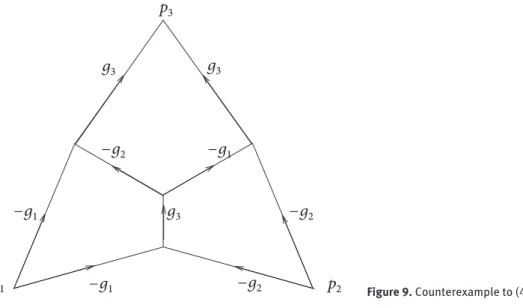
𝑝
1𝑝
2𝑝
3𝑝
0𝑔
3𝑔
1𝑔
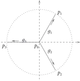
2Figure 3. Solution for the problem with boundary on the vertices of an equilateral triangle.
In Definition 3.1 we intentionally kept vague the regularity of the form 𝜔. Indeed 𝜔 has to be a compactly supported² smooth form, a priori, in order to fit Definition 1.5. Nevertheless, in some situations it will be useful to consider calibrations with lower regularity, for instance piecewise constant forms. As long as (3.1)–(3.4) remain valid, it is meaningful to do so; for this reason we introduce the following very general definition.
Definition 3.5. A generalized calibration associated with a 𝑘-dimensional normal 𝐸-current 𝑇 is a linear and
bounded functional 𝜙 on the space of normal 𝐸-currents satisfying the following conditions: (i) 𝜙(𝑇) = 𝕄(𝑇),
(ii) 𝜙(𝜕𝑅) = 0 for any (𝑘 + 1)-dimensional normal 𝐸-current 𝑅, (iii) ‖𝜙‖ ≤ 1.
Remark 3.6. Proposition 3.2 still holds, since for every competitor 𝑇with 𝜕𝑇 = 𝜕𝑇, there holds
𝕄(𝑇) = 𝜙(𝑇) = 𝜙(𝑇) + 𝜙(𝜕𝑅) ≤ 𝕄(𝑇),
where 𝑅 is chosen such that 𝑇 − 𝑇= 𝜕𝑅. Suchan𝑅 exists because 𝑇 and 𝑇are in the same homology class.
As examples, we present the calibrations for two well-known Steiner tree problems in ℝ2. Both “calibrations”
in Example 3.10 and in Example 3.11 are piecewise constant 1-forms (with values in normed vector spaces of dimension 3 and 6, respectively). So firstly we need to show that certain piecewise constant forms provide generalized calibrations in the sense of Definition 3.5.
Definition 3.7. Fix a 1-dimensional rectifiable 𝐺-current 𝑇 in ℝ2, 𝑇 = 𝑇(Σ, 𝜏, 𝜃). Assume we have a
collec-tion {𝐶𝑟}𝑟≥1which is a locally finite, Lipschitz partition of ℝ2, where the sets 𝐶𝑟have non-empty connected
interior, the boundary of every set 𝐶𝑟is a Lipschitz curve (of finite length, unless 𝐶𝑟is unbounded) and
𝐶𝑟∩ 𝐶𝑠= 0 whenever 𝑟 ̸= 𝑠. Assume moreover that 𝐶1is a closed set and for every 𝑟 > 1,
𝐶𝑟⊃ (𝐶𝑟\ ⋃ 𝑖<𝑟𝐶𝑖).
Let us consider a compactly supported piecewise constant 𝐸∗-valued 1-form 𝜔 with
𝜔 ≡ 𝜔𝑟 on 𝐶𝑟,
where 𝜔𝑟∈ Λ1𝐸(ℝ2) for every 𝑟. In particular 𝜔 ̸= 0 only on finitely many elements of the partition. Then we
say that 𝜔 represents a compatible calibration for 𝑇 if the following conditions hold:
2 Since we deal with currents that are compactly supported, we can easily drop the assumption that 𝜔 has compact support.
Figure 3. Solution for the problem with boundary on the vertices of an
equilateral triangle.
Example 3.4. Consider the vector space 𝐸 and the group 𝐺 defined in Lemma 2.6 with 𝑛 = 3; let 𝑝0= (0, 0), 𝑝1= (1/2, √3/2), 𝑝2= (1/2, −√3/2), 𝑝3= (−1, 0)
(see Figure 3). Consider the rectifiable 𝐺-current 𝑇 supported in the cone over (𝑝1, 𝑝2, 𝑝3), with respect to 𝑝0,
with piecewise constant weights 𝑔1, 𝑔2, 𝑔3:= −(𝑔1+ 𝑔2) on 𝑝0𝑝1, 𝑝0𝑝2, 𝑝0𝑝3respectively (see Figure 3 for the
orientation). This current 𝑇 is a minimizer for the mass. In fact, a constant 𝐺-calibration 𝜔 associated with 𝑇 is
𝜔 := (12d𝑥1+ √32 d𝑥2 1
2d𝑥1− √32 d𝑥2
) .
Condition (i) is easy to check and condition (ii) is trivially verified because 𝜔 is constant. To check condi-tion (iii) we note that, for the vector 𝜏 = cos 𝛼 e1+ sin 𝛼 e2, we have
⟨𝜔; 𝜏, ⋅ ⟩ = (12cos 𝛼 +√32 sin 𝛼 1
2cos 𝛼 −√32 sin 𝛼
) .
In order to compute the comass norm of 𝜔, we could use the characterization of the norm ‖ ⋅ ‖𝐸∗given in
Remark 2.7, but for 𝑛 = 3 computations are simpler. Since the unit ball of 𝐸 is convex, and its extreme points are the unit points of 𝐺, it is sufficient to evaluate ⟨𝜔; 𝜏, ⋅ ⟩ on ±𝑔1, ±𝑔2, ±(𝑔1+ 𝑔2). We have
|⟨𝜔; 𝜏, 𝑔1⟩| = |⟨𝜔; 𝜏, −𝑔1⟩| =sin(𝛼 +𝜋 6) ≤ 1, |⟨𝜔; 𝜏, 𝑔2⟩| = |⟨𝜔; 𝜏, −𝑔2⟩| =sin(𝛼 +5
6𝜋) ≤ 1, |⟨𝜔; 𝜏, 𝑔1+ 𝑔2⟩| = |⟨𝜔; 𝜏, −(𝑔1+ 𝑔2)⟩| = |cos 𝛼| ≤ 1.
In Definition 3.1 we intentionally kept vague the regularity of the form 𝜔. Indeed 𝜔 has to be a compactly supported² smooth form, a priori, in order to fit Definition 1.5. Nevertheless, in some situations it will be useful to consider calibrations with lower regularity, for instance piecewise constant forms. As long as (3.1)–(3.4) remain valid, it is meaningful to do so; for this reason we introduce the following very general definition. Definition 3.5. A generalized calibration associated with a 𝑘-dimensional normal 𝐸-current 𝑇 is a linear and bounded functional 𝜙 on the space of normal 𝐸-currents satisfying the following conditions:
(i) 𝜙(𝑇) = 𝕄(𝑇),
(ii) 𝜙(𝜕𝑅) = 0 for any (𝑘 + 1)-dimensional normal 𝐸-current 𝑅, (iii) ‖𝜙‖ ≤ 1.
Remark 3.6. Proposition 3.2 still holds, since for every competitor 𝑇with 𝜕𝑇 = 𝜕𝑇, there holds
𝕄(𝑇) = 𝜙(𝑇) = 𝜙(𝑇) + 𝜙(𝜕𝑅) ≤ 𝕄(𝑇),
where 𝑅 is chosen such that 𝑇 − 𝑇= 𝜕𝑅. Such an 𝑅 exists because 𝑇 and 𝑇are in the same homology class.
As examples, we present the calibrations for two well-known Steiner tree problems in ℝ2. Both “calibrations”
in Example 3.10 and in Example 3.11 are piecewise constant 1-forms (with values in normed vector spaces of dimension 3 and 6, respectively). So firstly we need to show that certain piecewise constant forms provide generalized calibrations in the sense of Definition 3.5.
Definition 3.7. Fix a 1-dimensional rectifiable 𝐺-current 𝑇 in ℝ2, 𝑇 = 𝑇(Σ, 𝜏, 𝜃). Assume we have a
collec-tion {𝐶𝑟}𝑟≥1which is a locally finite, Lipschitz partition of ℝ2, where the sets 𝐶𝑟have non-empty connected
interior, the boundary of every set 𝐶𝑟 is a Lipschitz curve (of finite length, unless 𝐶𝑟 is unbounded) and
𝐶𝑟∩ 𝐶𝑠= 0 whenever 𝑟 ̸= 𝑠. Assume moreover that 𝐶1is a closed set and for every 𝑟 > 1,
𝐶𝑟⊃ (𝐶𝑟\ ⋃ 𝑖<𝑟𝐶𝑖).
Let us consider a compactly supported piecewise constant 𝐸∗-valued 1-form 𝜔 with 𝜔 ≡ 𝜔
𝑟 on 𝐶𝑟, where
𝜔𝑟 ∈ Λ1𝐸(ℝ2) for every 𝑟. In particular 𝜔 ̸= 0 only on finitely many elements of the partition. Then we say that 𝜔
represents a compatible calibration for 𝑇 if the following conditions hold: (i) forH1-almost every point 𝑥 ∈ Σ, ⟨𝜔(𝑥); 𝜏(𝑥), 𝜃(𝑥)⟩ = ‖𝜃(𝑥)‖𝐸,
(ii) forH1-almost every point 𝑥 ∈ 𝜕𝐶𝑟∩ 𝜕𝐶𝑠we have
⟨𝜔𝑟− 𝜔𝑠; 𝜏(𝑥), ⋅ ⟩ = 0,
where 𝜏 is tangent to 𝜕𝐶𝑟,
(iii) ‖𝜔𝑟‖ ≤ 1 for every 𝑟.
We will refer to condition (ii) with the expression of compatibility condition for a piecewise constant form. Proposition 3.8. Let 𝜔 be a compatible calibration for the rectifiable 𝐺-current 𝑇. Then 𝑇 minimizes the mass among the normal 𝐸-currents with boundary 𝜕𝑇.
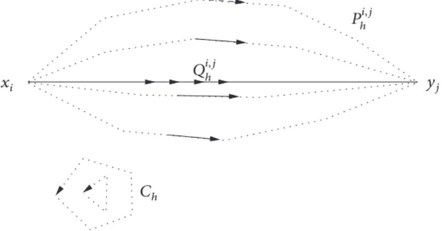
To prove this proposition we need the following result of decomposition of classical normal 1-currents, see [24] for the classical result and [21] for its generalization to metric spaces. Given a compact measure space (𝑋, 𝜇) and a family of 𝑘-currents {𝑇𝑥}𝑥∈𝑋in ℝ𝑑such that
∫ 𝑋 𝕄(𝑇𝑥) d𝜇(𝑥) < +∞, we denote by 𝑇 := ∫ 𝑋 𝑇𝑥d𝜇(𝑥)
the 𝑘-current 𝑇 satisfying
⟨𝑇, 𝜔⟩ = ∫
𝑋
⟨𝑇𝑥, 𝜔⟩ d𝜇(𝑥)
for every smooth compactly supported 𝑘-form 𝜔.
Proposition 3.9. Every normal 1-current 𝑇 in ℝ𝑑can be written as
𝑇 =
𝑀
∫
0
𝑇𝑡d𝑡,
where 𝑇𝑡is an integral current with 𝕄(𝑇𝑡) ≤ 2 and 𝕄(𝜕𝑇𝑡) ≤ 2 for every 𝑡, and 𝑀 is a positive number depending
only on 𝕄(𝑇) and 𝕄(𝜕𝑇). Moreover
𝕄(𝑇) =
𝑀
∫
0
30 | A. Marchese and A. Massaccesi, The Steiner tree problem revisited
Proof of Proposition 3.8. Firstly we see that a suitable counterpart of Stokes’ theorem holds. Namely, given a component 𝜔𝑗of 𝜔 and a classical integral 1-current 𝑇 = 𝑇(Σ, 𝜏, 1) in ℝ2, without boundary, then we claim
that
⟨𝜔𝑗; 𝑇⟩ := ∫
Σ
⟨𝜔𝑗(𝑥); 𝜏(𝑥)⟩ dH1(𝑥) = 0. (3.5)
To prove the claim, note that it is possible to find at most countably many unit multiplicity integral 1-currents 𝑇𝑖= 𝑇(Σ𝑖, 𝜏𝑖, 1) in ℝ2, without boundary, each one supported in a single set 𝐶
𝑟, such that ∑𝑖𝑇𝑖= 𝑇.
Since 𝜔𝑗≡ 𝜔𝑗
𝑟on 𝐶𝑟and since (ii) holds, we obtain
∫ Σ𝑖 ⟨𝜔𝑗(𝑥); 𝜏 𝑖(𝑥)⟩ dH1(𝑥) = ∫ Σ𝑖 ⟨𝜔𝑗 𝑟(𝑥); 𝜏𝑖(𝑥)⟩ dH1(𝑥) = 0
for every 𝑖; then the claim follows.
As a consequence of (3.5) we can find a family of “potentials”, i.e. Lipschitz functions 𝜙𝑗: ℝ2→ ℝ such
that for every (classical) integral 1-current 𝑆 associated to a Lipschitz path 𝛾 with 𝛾(1) = 𝑥𝑆and 𝛾(0) = 𝑦𝑆, there
holds
⟨𝜔𝑗; 𝑆⟩ = 𝜙𝑗(𝑥𝑆) − 𝜙𝑗(𝑦𝑆) for every 𝑗.
Indeed, by (3.5) the above integral does not depend on the path 𝛾 but only on the points 𝑥𝑆and 𝑦𝑆. Therefore,
in order to construct such potentials, it is sufficient to choose 𝜙𝑗(0) = 0 and
𝜙𝑗(𝑥) = |𝑥| 1
∫
0
⟨𝜔𝑗(𝑡𝑥); 𝑥|𝑥|⟩ d𝑡.
Moreover it is easy to see that every 𝜙𝑗is constant outside of the support of 𝜔𝑗, so we can assume, possibly
subtracting a constant, that 𝜙𝑗is compactly supported.
Now, consider any 2-dimensional normal 𝐸-current 𝑇. Let {𝑇𝑗}
𝑗be the components of 𝑇. For every 𝑗, use
Proposition 3.9 to write 𝑆𝑗:= 𝜕𝑇𝑗= 𝑀𝑗 ∫ 0 𝑆𝑗𝑡d𝑡. Then we have ⟨𝜔; 𝜕𝑇⟩ = ∑ 𝑗 𝑀𝑗 ∫ 0 ⟨𝜔𝑗; 𝑆𝑗𝑡⟩ d𝑡 = ∑ 𝑗 𝑀𝑗 ∫ 0 𝜙𝑗(𝑥𝑆𝑗𝑡) − 𝜙𝑗(𝑦𝑆𝑗𝑡) d𝑡.
Since for every 𝑗 we have
0 = 𝜕(𝜕𝑇𝑗) = 𝑀𝑗 ∫ 0 𝛿𝑥 𝑆𝑗𝑡− 𝛿𝑦𝑆𝑗𝑡d𝑡, it follows that 𝑀𝑗 ∫ 0 𝑔(𝑥𝑆𝑗 𝑡) − 𝑔(𝑦𝑆𝑗𝑡) d𝑡 = 0
for every 𝑗 and for every compactly supported Lipschitz function 𝑔, in particular for 𝑔 = 𝜙𝑗. Hence we
have ⟨𝜔; 𝜕𝑇⟩ = 0.
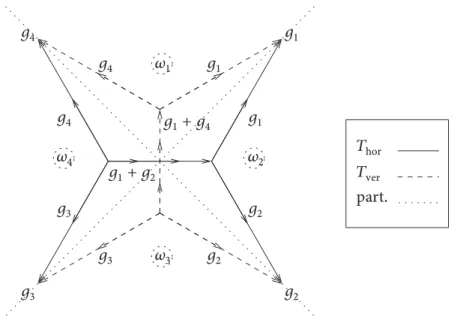
Example 3.10. Consider the points 𝑝1= (1, 1), 𝑝2= (1, −1), 𝑝3= (−1, −1), 𝑝4= (−1, 1) ∈ ℝ2. The corresponding
solution of the Steiner tree problem³ are those represented in Figure 1. We associate with each point 𝑝𝑗
with 𝑗 = 1, . . . , 4 the coefficients 𝑔𝑗∈ 𝐺, where 𝐺 is the group defined in Lemma 2.6 with 𝑛 = 4: let us call
𝐵 := 𝑔1𝛿𝑝1+ 𝑔2𝛿𝑝2+ 𝑔3𝛿𝑝3+ 𝑔4𝛿𝑝4.
3 In dimension 𝑑 > 2, an interesting question related to this problem is the following: is the cone over the (𝑑 − 2)-skeleton of
the hypercube in ℝ𝑑area minimizing, among hypersurfaces separating the faces? The question has a positive answer if and only
This 0-dimensional current is our boundary. Intuitively our mass-minimizing candidates among 1-dimen-sional rectifiable 𝐺-currents are those represented in Figure 4: these currents 𝑇hor, 𝑇verare supported in the
sets drawn, respectively, with continuous and dashed lines in Figure 4 and have piecewise constant coeffi-cients intended to satisfy the boundary condition 𝜕𝑇14 | A. Marchese and A. Massaccesi, The Steiner tree problem revisitedhor= 𝐵 = 𝜕𝑇ver.
𝑔
1𝑔
2𝑔
3𝑔
4𝑔
1𝑔
4𝑔
2𝑔
1+ 𝑔
2𝑔
1+ 𝑔
4𝑔
1𝑔
4𝑔
3𝑔
3𝑔
2𝑇
ver𝜔
1𝜔
3𝜔
2𝜔
4𝑇
horpart.
Figure 4. Solution for the mass-minimization problem.
It is easy to check that 𝜔 satisfies both condition (i) and the compatibility condition of Definition 3.7. To check that condition (iii) is satisfied, we can use formula (2.5).
Example 3.11. Consider the vertices of a regular hexagon plus the center, namely
𝑝1= (1/2, √3/2), 𝑝2= (1, 0), 𝑝3= (1/2, −√3/2),
𝑝4= (−1/2, −√3/2), 𝑝5= (−1, 0), 𝑝6= (−1/2, √3/2), 𝑝7= (0, 0),
and associate with each point 𝑝𝑗the corresponding multiplicity 𝑔𝑗∈ 𝐺, where 𝐺 is the group defined in
Lemma 2.6 with 𝑛 = 4. A mass-minimizer for the problem with boundary 𝐵 =∑7
𝑗=1𝑔𝑗𝛿𝑝𝑗
is illustrated in Figure 5, the other one can be obtained with a 𝜋/3-rotation of the picture.
Figure 5. Solution for the mass-minimization problem.
Let us divide ℝ2intosix cones of angle 𝜋/3, as in Figure 5; we will label each cone with a number
from 1 to 6, starting from that containing (0, 1) and moving clockwise. A compatible calibration for the two
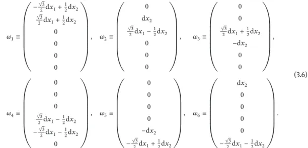
minimizers is the following: Note 4:
Display: Shall I replace = by :=?
Figure 4. Solution for the mass-minimization problem.
In this case, a compatible calibration for both 𝑇horand 𝑇veris defined piecewise as follows (the notation
is the same as in Example 3.4 and the partition is delimited by the dotted lines): 𝜔1≡ ( √3 2 d𝑥1+ 12d𝑥2 (1 −√32 )d𝑥1−12d𝑥2 (−1 +√32 )d𝑥1−1 2d𝑥2 ) , 𝜔2≡ ( 1 2d𝑥1+ √32d𝑥2 1 2d𝑥1− √32d𝑥2 −1 2d𝑥1− (1 −√32 )d𝑥2 ) , 𝜔3≡ ( (1 −√32)d𝑥1+ 12d𝑥2 √3 2d𝑥1−12d𝑥2 −√32 d𝑥1− 12d𝑥2 ) , 𝜔4≡ ( 1 2d𝑥1+ (1 −√32)d𝑥2 1 2d𝑥1− (1 −√32)d𝑥2 −1 2d𝑥1− √32d𝑥2 ) .
It is easy to check that 𝜔 satisfies both condition (i) and the compatibility condition of Definition 3.7. To check that condition (iii) is satisfied, we can use formula (2.5).
Example 3.11. Consider the vertices of a regular hexagon plus the center, namely 𝑝1= (1/2, √3/2), 𝑝2= (1, 0),
𝑝3= (1/2, −√3/2), 𝑝4= (−1/2, −√3/2),
𝑝5= (−1, 0), 𝑝6= (−1/2, √3/2),
𝑝7= (0, 0),
and associate with each point 𝑝𝑗 the corresponding multiplicity 𝑔𝑗∈ 𝐺, where 𝐺 is the group defined in
Lemma 2.6 with 𝑛 = 4. A mass-minimizer for the problem with boundary 𝐵 =∑7
𝑗=1𝑔𝑗𝛿𝑝𝑗
32 | A. Marchese and A. Massaccesi, The Steiner tree problem revisitedA. Marchese and A. Massaccesi, The Steiner tree problem revisited | 15
𝑔
1𝑔
6𝑔
2𝑔
3𝑔
4𝑔
5𝑔
7Figure 5. Solution for the mass-minimization problem.
Again, it is not difficult to check that 𝜔 satisfies both condition (i) and the compatibility condition of Definition 3.7. To check that condition (iii) is satisfied, we use formula (2.5).
Remark 3.12. We may wonder whether or not the calibration given in Example 3.11 can be adjusted so to work
for the set of the vertices of the hexagon (without the seventh point in the center): the answer is negative, in fact the support of the current in Figure 5 is not a solution for the Steiner tree problem on the six points, the perimeter of the hexagon minus one side being the shortest graph, as proved in [15].
Remark 3.13. In both Examples 3.10 and 3.11, once we fixed the partition and we decided to look for a
piece-wise constant calibration for our candidates, the construction of 𝜔 was forced by both conditions (i) of Definition 3.1 and the compatibility condition of Definition 3.7. Notice that the calibration for Example 3.11 has evident analogies with the one exhibited in Example 3.4. Actually we obtained the first one simply pasting suitably “rotated” copies of the second one.
In the following remarks we intend to underline the analogies and the connections with calibrations in similar contexts. See [20, Chapter 6] for an overview on the subject of calibrations.
Remark 3.14 (Functionals defined on partitions and null lagrangians). There is an interesting and deep
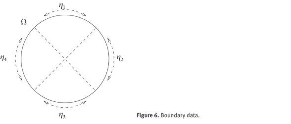
anal-ogy between calibrations and null lagrangians, analanal-ogy that still holds in the group-valued coefficients framework. Consider some points {𝜂1, . . . , 𝜂𝑛} ⊂ ℝ𝑚with
|𝜂𝑖− 𝜂𝑗| = 1 for all 𝑖 ̸= 𝑗, (3.7)
and fix an open set with Lipschitz boundary Ω ⊂ ℝ𝑑. It is natural to study the variational problem
inf{∫
Ω
|𝐷𝑢| : 𝑢 ∈ BV(Ω; {𝜂1, . . . , 𝜂𝑛}), 𝑢|𝜕Ω≡ 𝑢0}. (3.8)
It turns out that ∫Ω|𝐷𝑢| is the same energy we want to minimize in the Steiner tree problem, ∫Ω|𝐷𝑢| being the length of the jump set of 𝑢.
This problem concerns the theory of partitions of an open set Ω in a finite number of sets of finite perimeter. This theory was developed by Ambrosio and Braides in [1, 2], which we refer to for a complete exposition.
Figure 5. Solution for the mass-minimization problem. Let us divide ℝ2 into six cones of angle 𝜋/3, as in Figure 5; we will label each cone with a number
from 1 to 6, starting from that containing (0, 1) and moving clockwise. A compatible calibration for the two minimizers is the following:
𝜔1≡ ( ( ( ( ( ( ( −√32 d𝑥1+ 1 2d𝑥2 √3 2d𝑥1+12d𝑥2 0 0 0 0 ) ) ) ) ) ) ) , 𝜔2≡ ( ( ( ( ( ( ( 0 d𝑥2 √3 2 d𝑥1− 12d𝑥2 0 0 0 ) ) ) ) ) ) ) , 𝜔3≡ ( ( ( ( ( ( ( 0 0 √3 2d𝑥1+12d𝑥2 −d𝑥2 0 0 ) ) ) ) ) ) ) , 𝜔4≡ ( ( ( ( ( ( ( 0 0 0 √3 2d𝑥1−12d𝑥2 −√32 d𝑥1− 12d𝑥2 0 ) ) ) ) ) ) ) , 𝜔5≡ ( ( ( ( ( ( ( 0 0 0 0 −d𝑥2 −√32d𝑥1+1 2d𝑥2 ) ) ) ) ) ) ) , 𝜔6≡ ( ( ( ( ( ( ( d𝑥2 0 0 0 0 −√32 d𝑥1− 1 2d𝑥2 ) ) ) ) ) ) ) . (3.6)
Again, it is not difficult to check that 𝜔 satisfies both condition (i) and the compatibility condition of Definition 3.7. To check that condition (iii) is satisfied, we use formula (2.5).
Remark 3.12. We may wonder whether or not the calibration given in Example 3.11 can be adjusted so to work for the set of the vertices of the hexagon (without the seventh point in the center): the answer is negative, in fact the support of the current in Figure 5 is not a solution for the Steiner tree problem on the six points, the perimeter of the hexagon minus one side being the shortest graph, as proved in [15].
Remark 3.13. In both Examples 3.10 and 3.11, once we fixed the partition and we decided to look for a piece-wise constant calibration for our candidates, the construction of 𝜔 was forced by both conditions (i) of Definition 3.1 and the compatibility condition of Definition 3.7. Notice that the calibration for Example 3.11 has evident analogies with the one exhibited in Example 3.4. Actually we obtained the first one simply pasting suitably “rotated” copies of the second one.
In the following remarks we intend to underline the analogies and the connections with calibrations in similar contexts. See [20, Chapter 6] for an overview on the subject of calibrations.
Remark 3.14 (Functionals defined on partitions and null lagrangians). There is an interesting and deep anal-ogy between calibrations and null lagrangians, analanal-ogy that still holds in the group-valued coefficients
framework. Consider some points {𝜂1, . . . , 𝜂𝑛} ⊂ ℝ𝑚with
|𝜂𝑖− 𝜂𝑗| = 1 for all 𝑖 ̸= 𝑗, (3.7)
and fix an open set with Lipschitz boundary Ω ⊂ ℝ𝑑. It is natural to study the variational problem
inf{∫
Ω
|𝐷𝑢| : 𝑢 ∈ BV(Ω; {𝜂1, . . . , 𝜂𝑛}), 𝑢|𝜕Ω ≡ 𝑢0}. (3.8)
It turns out that ∫Ω|𝐷𝑢| is the same energy we want to minimize in the Steiner tree problem, ∫Ω|𝐷𝑢| being the length of the jump set of 𝑢.16 | A. Marchese and A. Massaccesi, The Steiner tree problem revisited
𝜂
4𝜂
2𝜂
1𝜂
3Ω
Figure 6. Boundary data.
Remark 3.15 (Clusters with multiplicities). In [19], F. Morgan applies flat chains with coefficients in a group 𝐺
to soap bubble clusters and immiscible fluids, following the idea of B. White in [25]. For a detailed comparison of [19] with our technique, see [18,Section3.2.3]. Here we just notice that the definition of calibration in [19] works well in the case of free abelian groups and this is the main difference with our approach.
Remark 3.16 (Paired calibrations). It is worth mentioning another analogy between the technique of
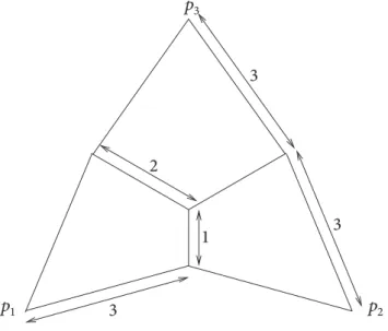
cal-ibrations (for currents with coefficients in a group) illustrated in this paper and the technique of paired calibrations in [17]. In particular, in the specific example of the truncated cone over the 1-skeleton of the tetrahedron in ℝ3(the surface with least area among those separating the faces of the tetrahedron), one can
detect a correspondence even at the level of the main computations. See [18,Section3.2.3] for the details. Following an idea of Federer (see [11]), in [17, 19] (and in [5, 6], as well) one can observe the exploitation of the duality between minimal surfaces and maximal flows through the same boundary. We will examine this duality in Section 4, but we conclude the present section with a remark closely related to this idea.
Remark 3.17 (Covering spaces and calibrations for soap films). In [6] Brakke develops new tools in
Geomet-ric Measure Theory for the analysis of soap films: as the underlying physical problem suggests, one can represent a soap film as the superposition of two oppositely oriented currents. In order to avoid cancellations of multiplicities, the currents are defined in a covering space and, as stated in [6], the calibration technique still holds.
Let us remark that cancellations between multiplicities were a significant obstacle for the Steiner tree problem, too. The representation of currents in a covering space goes in the same direction of currents with coefficients in a group, though, as in Remark 3.16, a sort of Poincaré duality occurs in the formulation of the Steiner tree problem (1-dimensional currents in ℝ𝑑) with respect to the soap film problem (currents of
codimension 1 in ℝ𝑑).
4 Existence of the calibration and open problems
Once we established that the existence of a calibration is a sufficient condition for a rectifiable 𝐺-current to be a mass-minimizer, we may wonder if the converse is also true: does a calibration (of some sort) exist for
Figure 6. Boundary data.
This problem concerns the theory of partitions of an open set Ω in a finite number of sets of finite perimeter. This theory was developed by Ambrosio and Braides in [1, 2], which we refer to for a complete exposition.
The analog of a calibration in this context is a null lagrangian⁴ with some special properties: again, the existence of such an object, associated with a function 𝑢, is a sufficient condition for 𝑢 to be a minimizer for the variational problem (3.8) with a given boundary condition.
We refer to [18, Section 3.2.4] for a detailed survey of the analogy.
Remark 3.15 (Clusters with multiplicities). In [19], F. Morgan applies flat chains with coefficients in a group 𝐺 to soap bubble clusters and immiscible fluids, following the idea of B. White in [25]. For a detailed comparison of [19] with our technique, see [18, Section 3.2.3]. Here we just notice that the definition of calibration in [19] works well in the case of free abelian groups and this is the main difference with our approach.
Remark 3.16 (Paired calibrations). It is worth mentioning another analogy between the technique of cal-ibrations (for currents with coefficients in a group) illustrated in this paper and the technique of paired calibrations in [17]. In particular, in the specific example of the truncated cone over the 1-skeleton of the tetrahedron in ℝ3(the surface with least area among those separating the faces of the tetrahedron), one can
detect a correspondence even at the level of the main computations. See [18, Section 3.2.3] for the details. Following an idea of Federer (see [11]), in [17, 19] (and in [5, 6], as well) one can observe the exploitation of the duality between minimal surfaces and maximal flows through the same boundary. We will examine this duality in Section 4, but we conclude the present section with a remark closely related to this idea.
Remark 3.17 (Covering spaces and calibrations for soap films). In [6] Brakke develops new tools in Geomet-ric Measure Theory for the analysis of soap films: as the underlying physical problem suggests, one can 4 See [7] for an overview on null lagrangians.
34 | A. Marchese and A. Massaccesi, The Steiner tree problem revisited
represent a soap film as the superposition of two oppositely oriented currents. In order to avoid cancellations of multiplicities, the currents are defined in a covering space and, as stated in [6], the calibration technique still holds.
Let us remark that cancellations between multiplicities were a significant obstacle for the Steiner tree problem, too. The representation of currents in a covering space goes in the same direction of currents with coefficients in a group, though, as in Remark 3.16, a sort of Poincaré duality occurs in the formulation of the Steiner tree problem (1-dimensional currents in ℝ𝑑) with respect to the soap film problem (currents of
codimension 1 in ℝ𝑑).
4 Existence of the calibration and open problems
Once we established that the existence of a calibration is a sufficient condition for a rectifiable 𝐺-current to be a mass-minimizer, we may wonder if the converse is also true: does a calibration (of some sort) exist for every mass-minimizing rectifiable 𝐺-current?
Let us step backward: does it occur for classical integral currents? The answer is quite articulate, but we can briefly summarize the state of the art we will rely upon.
We consider a boundary 𝐵0, that is, a (𝑘 − 1)-dimensional rectifiable 𝐺-current without boundary, and
we compare the following minima:
M𝐸(𝐵0) := min{𝕄(𝑇) : 𝑇 is a normal 𝑘-dimensional 𝐸-current, 𝜕𝑇 = 𝐵0}
and
M𝐺(𝐵0) := min{𝕄(𝑇) : 𝑇 is a rectifiable 𝑘-dimensional 𝐺-current, 𝜕𝑇 = 𝐵0}.
ObviouslyM𝐸(𝐵0) ≤M𝐺(𝐵0), the main issue is to establish whether they coincide or not. In fact, a normal
𝐸-current 𝑇 with boundary 𝐵0admits a generalized calibration if and only if 𝕄(𝑇) =M𝐸(𝐵0), as we recall in
Proposition 4.2. In the classical case (𝐸 = ℝ and 𝐺 = ℤ) it is known that
(i) Mℝ(𝐵0) may be strictly less thanMℤ(𝐵0) (and, if this happens, a solution forMℤ(𝐵0) cannot be
cali-brated),
(ii) Mℤ(𝐵0) =Mℝ(𝐵0) if 𝑘 = 1, as we prove in Proposition 4.3.
At the end of this section, we show that this outlook changes significantly when we replace the ambient space ℝ𝑑with a suitable metric space.
Remark 4.1. For every mass-minimizing classical normal 𝑘-current 𝑇, there exists a generalized calibration 𝜙 in the sense of Definition 3.5. Moreover, by means of the Riesz Representation Theorem, 𝜙 can be represented by a measurable map from 𝑈 to Λ𝑘(ℝ𝑑). This result is contained in [11].
In particular, Remark 4.1 provides a positive answer to the question of the existence of a generalized cali-bration for mass-minimizing integral currents of dimension 𝑘 = 1, because minima among both normal and integral currents coincide, as we prove in Proposition 4.3. It is possible to apply the same technique in the class of normal 𝐸-currents, therefore we have the following proposition.
Proposition 4.2. For every mass-minimizing normal 𝐸-current 𝑇, there exists a generalized calibration. The following fact is probably in the folklore, unfortunately we were not able to find any literature on it. We give a proof here in order to enlighten the problems arising in the case of currents with coefficients in a group.
Proposition 4.3. Consider the boundary of an integral 1-current in ℝ𝑑, represented as
𝐵0= − 𝑁− ∑ 𝑖=1𝑎𝑖𝛿𝑥𝑖+ 𝑁+ ∑ 𝑗=1𝑏𝑗𝛿𝑦𝑗, 𝑎𝑖, 𝑏𝑗 ∈ ℕ. (4.1) ThenMℝ(𝐵0) =Mℤ(𝐵0).