Design, build and test of an axial flow hydrokinetic turbine with fatigue analysis

(1)

Design, Build and Test of an Axial Flow Hydrokinetic Turbine with Fatigue Analysis by

Jerod W. Ketcham B.S., Mechanical Engineering Wichita State University, 1997

Submitted to the Department of Mechanical Engineering and the Department of Materials Science and Engineering in Partial Fulfillment of the Requirements for the Degrees of

Naval Engineer and

Master of Science in Materials Science and Engineering at the Massachusetts Institute of Technology

June 2010

Signature of Author

SEP 0

1 2010

LIBRARIES

Delartme ot Mechanical Engineerng

May 7 1,fl111

Mark S. Welsh Professor of the Practice of Naval Architecture and Engineering

/Thesis Supervisor

Richard W. Kimball Thesis Supervisor Certified by

Professor of Materials Science and Engineering and Nuclear

Accepted by

Ronald G. Ballinger Science and Engineering T gakpervisor -David E. Hardt tee o radu ents Me ical nn ering

Chair, Departmental Committee on Gradut e nts Department of Materials Science and Engin ing Certified by

Certified by

(2)

Design, Build and Test of an Axial Flow Hydrokinetic Turbine with Fatigue Analysis by

Jerod W. Ketcham

Submitted to the Department of Mechanical Engineering and the Department of Materials Science and Engineering on May 7, 2010 in partial fulfillment of the requirements for the degrees of Naval Engineer and Master of Science in Materials Science and Engineering

Abstract

OpenProp is an open source propeller and turbine design and analysis code that has been in development since 2007 by MIT graduate students under the supervision of Professor Richard Kimball. In order to test the performance predictions of OpenProp for axial flow hydrokinetic turbines, a test fixture was designed and constructed, and a model scale turbine was tested. Tests were conducted in the MIT water tunnel for tip speed ratios ranging from 1.55 to 7.73.

Additional code was also written and added to OpenProp in order to implement ABS steel vessels rules for propellers and calculate blade stress. The blade stress code was used to conduct a fatigue analysis for a model scale propeller using a quasi-steady approach.

Turbine test results showed that OpenProp provides good performance predictions for the on-design operational condition but that further work is needed to improve performance predictions for the off-design operational condition. Fatigue analysis results show that reasonable estimates of propeller blade fatigue life can be obtained using a relatively simple method. Calculated blade stress distributions agree with previously published data obtained with more sophisticated and time consuming calculation techniques.

Thesis Supervisor: Mark S. Welsh

Title: Professor of the Practice of Naval Architecture and Engineering Thesis Supervisor: Richard W. Kimball

Thesis Supervisor: Ronald G. Ballinger

(3)

Acknowledgements

The author thanks the following individuals for their assistance in completing this thesis: Professor Rich Kimball for his advice and guidance on this project. His enthusiasm for this project and practical advice were greatly appreciated.

Professor Chryssostomos Chryssostomidis for his interest and financial support for this project. Without funding this project would have been impossible. I am grateful for his patience and understanding when things did not always go according to plan.

Dr. Brenden Epps for his assistance with the MATLAB@ code, work to restore the water tunnel and discussions where I could ask the simple questions. The duration of this project would have exceeded the time available without his help.

CAPT Mark Welsh for his leadership of the 2N program and encouragement during this project. Professor Ron Ballinger for his practical insight and level of interest in this project. Fatigue analysis is a tricky subject and could not have been navigated without his assistance.

Most importantly, my family, Jill, Justin, Jessica, Jason and Janae, for all their support and encouragement. The long and sometimes frustrating days would not have been possible without their full support.

(4)

TABLE OF FIGURES

Figure 1: Turbine Drawing Courtesy ofEpps... 11

F igure 2 : T urbine T est ... 11

Figure 3: Thrust C alibration... 12

Figure 4: Torque C alibration ... 13

Figure 5: Spectrum Analysis-600RPM, 1.69m/s ... 13

Figure 6: Friction T orque... 14

Figure 7: Measured Torque - No Correction... 14

Figure 8: Test Section Flow Speed Determination... 16

F igu re 9 : R esu lts ... 16

Figure 10: Blade Section with Lift and Flow Velocity Vectors ... 21

Figure 11: Blade Section Showing Lift Resolved into Axial and Tangential Components ... 22

Figure 12: Bending Moments Components ... 23

Figure 13: Total Bending Moments about Centroidal Axes... 24

Figure 14: Example Propeller Courtesy of Epps... 25

Figure 15: Distorted Root Section ... 25

Figure 16: Undistorted Root Section ... 26

Figure 17: Calculation of Elemental Area Properties ... 26

Figure 18: On-design Root Section Stress... 27

Figure 19: On-design Suction Side Stress: J=O. 75, Vs=1.5m/s, n=8rev/s, D=0.25m... 28

Figure 20: On-design Pressure Side Stress: J=O. 75, Vs=1.5m/s, n=8rev/s, D=0.25m ... 28

Figure 21: Off-design Suction Side Stress: J=0.40, Vs=1.5m/s, n=15rev/s, D=0.25m ... 29

Figure 22: Off-design Pressure Side Stress: J=0.40, Vs=1.5m/s, n=15rev/s, D=0.25m... 29

Figure 23: Sectored, Single Screw Ship Wake ... 32

Figure 24: Original Inflow Velocities... 32

Figure 25: New Inflow Velocities... 32

Figure 26: Pressure Side Blade Stress for Each Wake Sector ... 33

Figure 27: Point of Maximum Tensile Stress ... 34

Figure 28: Maximum Blade Stress versus Angular Position for Various Ship Speeds Using the On-Design Advance Coefficient (J=O. 75)... 35

Figure 29: S-N Curve for NiAl Bronze ... 36

Figure 30: Operational Profile for DDG51... 36

Figure 31: Example Operational Profile Used for Calculations ... 37

Figure 32: Time at Various Stress Levels... 37

Figure 33: Provided Sensor... 41

Figure 34: Stress from Axial Load on Sensor (501bf applied)... 41

Figure 35: Stress from Torque Load on Sensor (12ft-lbf applied) ... 42

Figure 36: Output Shaft Configuration... 43

Figure 37: Driveshaft and Bearing Assembly with Brush Blocks and Slip Rings ... 44

Figure 38: Installed Slip Rings and Brushes... 45

Figure 39: K089300-7Y Torque Speed Curve... 47

Figure 40: Output Power Capability ... 48

Figure 41: L im iting Current... 48

Figure 42: Electrical Components ... 50

Figure 43: Schematic of Enclosure Electrical Components ... 51

(6)

TABLE OF TABLES

Table 1: Development History of OpenProp ... 8

Table 2: Key Turbine Parameters ... 11

Table 3: Test Tip Speed Ratios... 15

Table 4: Test Fixture Limitations ... 40

(7)

Introduction

Since 2007, graduate students at the Massachusetts Institute of Technology (MIT) have been developing an open source propeller and turbine design and analysis tool under the supervision of Professor Richard Kimball. The tool is a set of open source MATLAB@ scripts published under the GNU General Public License which are capable of performing design and analysis studies for open and ducted propellers as well as axial flow turbines. This suite of MATLAB@ scripts is called OpenProp. OpenProp propeller design capabilities include performing

parametric studies of propellers using various propeller diameters, number of blades and rotation speeds. Propeller analysis features include performing off-design and cavitation analyses. A gap in OpenProp capabilities was the inability to evaluate the structural adequacy of a propeller or turbine. This project added two new modules. One module implements American Bureau of Shipping (ABS) steel vessel rules for propellers and the other calculates the blade surface stress. Validation of OpenProp turbine and propeller performance predictions is limited. The portion of the code suite which designs ducted propellers has been validated against the US Navy's

Propeller Lifting Line (PLL) code with excellent correlation. Several experiments have been done to validate open propeller performance predictions using a modified trolling motor

apparatus. One test had been performed, with limited success, of an axial flow turbine. No tests had been performed for ducted propellers. Because of this lack of experimental validation of OpenProp, it became necessary to design and construct a propeller and turbine test fixture that is robust and can easily be used to test open and ducted propellers as well as turbines. This project provided a test fixture, funded by MIT SeaGrant, which can be used in a water tunnel or tow tank to provide experimental performance results which can be used to validate OpenProp

performance predictions.

OpenProp implements the vortex lifting line method to quickly achieve a propeller or axial flow turbine design. The lifting line method of propeller design has some limitations but is an

excellent method to obtain an initial design which can be refined using more sophisticated design techniques. In the spirit of providing initial design estimates, this project also completed a

quasi-steady fatigue analysis and predicted the fatigue life of a propeller.

(8)

Chapter 1 -Development, Capability and Limitations of OpenProp

Development of OpenProp

OpenProp had its genesis in a code called MATLAB@ Propeller Vortex Lattice (MPVL) which was a code which added graphical user interfaces to Propeller Vortex Lattice (PVL) which was developed by Kerwin (2007) for his propellers course at the Massachusetts Institute of

Technology (MIT). Since that time significant capability has been added to the code and additional features and capability are being developed.

OpenProp uses a lifting line method to model blade circulation (Kerwin 2007). The lifting line technique has been well established and was implemented by Kerwin for preliminary parametric propeller design for the US Navy in a code called PLL. OpenProp development sought to expand and enhance the capabilities of Kerwin's code and make the software more user friendly. A full explanation for the theory of operation of OpenProp has been given by Epps (201 Ob).

Capability of OpenProp

A table showing the develop ent history and current capability of OpenProp is shown below.

Date Event Persons Description

Responsible

2001 PVL Developed J.E. Kerwin Lifting line design code used for Kerwin's

propeller class at MIT

2007 MPVL Developed H. Chung MATLAB@ version of PVL which

(Later renamed K.P. D'Epagnier incorporated GUIs for parametric and blade OpenProp v1.0) row design and geometry routines for CAD

(Rhino) interface. This code used a Lerb's criteria optimizer. Chung (2007),

D'Epagnier (2007)

2008 Cavitation Analysis C.J. Peterson Using Drela's XFOIL, routines and

Routines executables were developed for conducting

Developed propeller cavitation analysis, Peterson

(2008).

2008 OpenProp v2.0 J.M. Stubblefield Added capability for ducted propeller design

Stubblefield (2008)

2009 OpenProp v2.3 B.P. Epps Added new optimizer. Incorporated routines of Peterson, added off-design analysis, corrected errors and added ability to design axial flow turbines with or without blade chord optimization. Theory described in

Epps (2010b).

2010 Contra-Rotating D. Laskos Added the capability for contra-rotating Propeller Design propeller design with cavitation analysis.

Laskos (2010)

(9)

This project added the capability to calculate blade stress and implement ABS rules for

propellers. Epps continues to refine and expand OpenProp capabilities and is currently working on codes to predict propeller performance during shaft reversals.

Limitations of OpenProp

OpenProp uses the lifting line method to model the blade circulation. There are limits in regard to using this method in propeller design.

1. Constant Radius Vortex Helix - In the implementation of the lifting line method, the trailing vorticity is assumed to be of constant radius. For propellers, it is known that the trailing vorticity helix radius actually decreases. This simplification has been made to ease the complexity of calculating the influence of the trailing vorticity on the blade itself. The errors introduced with this simplification are relatively minor as shown in the

experimental data comparison in this paper and by Stubblefield (2008) in his comparison of OpenProp predictions to a more established propeller design code.

2. Skew and Rake - OpenProp does not allow the designer to design blades with skew or rake

3. 3D Lifting Surface Effects - By its very nature a design tool based on the lifting line method cannot account for the 3D lifting surface effects. The result is that the translation from calculated hydrodynamic characteristics to a blade geometry which produces the desired hydrodynamic performance is difficult and in most cases will contain errors. Therefore, the blade geometry that is generated from a lifting line code is an

approximation and one should not expect the propeller performance measured by experiment to completely match the lifting line predicted performance. A comparison and discussion of predicted performance versus experimental performance for U.S. Navy

(10)

Chapter 2 - Hydrokinetic Turbine Design and Construction

In propeller design the overall objective is to generate a specified thrust while minimizing the torque required to produce it. In turbine design the goal is to maximize the torque and minimize the thrust. A procedure which can be used with OpenProp for turbine design is:

1. Determine expected CD and CL. Typical ranges for these quantities are 0.008<CD<0.03 and 0.2<CL<0.5. The actual values for these parameters are dictated by the choice of blade section shape, flow regime and the degree of blade section scaling.

2. Perform parametric design study using expected CD/CL to determine number of blades and tip speed ratio. A typical value for this ratio is 0.06.

3. Select a design point from the parametric study of step 2. The turbine design point is characterized by the number of turbine blades and the tip speed ratio. In general, the more blades that a turbine has the greater its efficiency. However, in actual application this must be balanced by the manufacture costs of the turbine.

4. Choose the turbine diameter, free stream flow speed and rotation rate consistent with the chosen tip speed ratio in step 3 above such that desired power is achieved. Maximum turbine diameter is dictated by the water depth and installation scheme where the turbine will operate. It is generally desirable to maximize the turbine diameter in order to maximize the turbine's power capacity. Free stream flow speed is determined by the flow where the turbine will be installed. Desired rotation rate will be effected by the electrical generator selected for use with the turbine.

5. Perform an off-design performance analysis. An off-design performance analysis is necessary to obtain an overall picture of the time average power that the turbine will produce. This analysis is especially important for tidal turbines where there is a

fluctuation of flow speed.

6. Determine the span-wise blade chord and thickness distribution. This step is where the blade geometry is determined to produce the characteristics determined in the previous

steps. OpenProp can perform this step automatically by using the chord optimizer. 7. Perform blade stress analysis. A blade stress analysis is necessary to ensure the structural

adequacy of the blades.

The above procedure was used to design the turbine which was tested by Epps. Results are shown in Epps (2010a). The same turbine was retested as part of this project. Step 7 was not performed as part of the design process because the stress module of OpenProp was not available at that time. The turbine diameter was selected as the maximum diameter which could be

manufactured using the available rapid prototyping equipment and tested in the water tunnel test section. The number of blades was also dictated by the desire to maximize the turbine diameter and two blades were selected.

Epps (201 Oa) describes the procedure implemented in OpenProp to conduct a parametric design study, optimize a single turbine design and perform off-design analysis. For turbines the method can be summarized as setting the blade circulation less than zero and then simultaneously solving a set of equations such that the resulting variables represent a physically realizable condition. Epps (2009, 201 Oa) also discusses the correct way to optimize a turbine design.

(11)

Once the turbine was designed, the geometry module of OpenProp was used to create the set of points that represent the blade surface in three dimensions. This set of points was loaded into SolidWorks@ via a macro developed for this purpose. In SolidWorks®, the blade geometry was turned into a solid which was multiplied into two blades and attached to a hub. This file was saved in .stl format and loaded into the rapid prototyping machine for production. The model scale turbine that was generated in this way was tested by Epps and as part of this project. Turbine test results are presented in the next section.

Table 9.1 of Epps (201 Oa, p. 280) contains the turbine design parameters. That table is reproduced here in Table 2.

Parameter Value Description

Z 2 Number of blades

n 19.1 rev/s Rotation rate

D 0.25 m Diameter

Vs 3 m/s Free stream speed

Dhub 0.08382 _{Hub diameter}

M 20 Number of panels

p 1000 kg/m3 Water density

X 5 Tip speed ratio

CL,max 0.5 Maximum allowable lift coefficient

Table 2: Key Turbine Parameters

Figure 1: Turbine Drawing

Courtesy of Epps Figure 2: Turbine Test

(12)

Chapter 3 - Test Procedure, Results and Comparison

Test Procedure

Turbine testing was performed on a test fixture specifically designed for this purpose. The test fixture was funded via MIT SeaGrant and its design and construction are described in Chapter 7. Generally the test procedure consisted of measuring the shaft torque created by the turbine for various rotation rates and flow speeds. A detailed test procedure follows with test points in

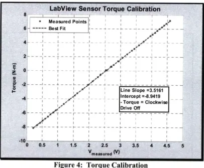
Table 3 and test results in Figure 9. Calibration

Calibration of the test fixture was performed by hanging known weights from the output shaft of the test fixture and reading strain gage amplifier output voltage using LabView@. This

calibration technique is a static calibration; a better calibration technique for this type of testing would have been a dynamic calibration. However, a dynamic calibration is more complicated and requires additional equipment which was unavailable. LabView® was connected to the test fixture in an identical way for both calibration and testing. Results of the calibration are shown Figure 3 and Figure 4.

LabView Sensor Thrust Calibration 2W 1 1 1 e Measured Points 5 i 1 --- Best Fit g I - Drive Off I I Drive Enabled 10 -% -- -4 50-- 50-- - Line Slope'-120.6234 - ~ ~ Intercept =319.51571 - Thrust = Compresion 1 1 F50igur 3 T CLibrio -n 1 1. -5 3 35 . -1001" M

(13)

LabView Sensor Torque Calibration g- - r i r -Measured Points I 5 6- BestFit ---- -- --- - -L -F - - L - 5 L T- --- -- -- - - -- - - -- - -0 _{Line Slope =3.5161} 4Intercept =-8.9419 - Torque = Clockwis Drive Off 7 F -- - 7 --- r-4 ---

F-Figure 4: Torque Calibration

Because the motor drive used for these tests uses pulse width modulation (PWM) at 300VDC and because the signal wires are running alongside the power cable (inside the same 1.5 inch

diameter standpipe) there was a concern that the Signal to Noise Ratio (SNR) would be too small

to be able to effectively measure the signal voltage. This concern was allayed by performing spectral analyses on the measured signal. A typical result of these analyses is shown in Figure 5.

The graph shows that there is minimal interference.

Welch Power Spectral Density Estimate -Torque

10 0 A 1-1.692m/sI 10600RPMI -10 -20 --3 - - -40 - -- K- - -so;-*0 -o -- - , t F-F-I F -F F- -7 -7, F F

Figure 5: Spectrum Analysis-600RPM, 1.69m/s

Since the calibration that was used was a static calibration, it is necessary to correct the measured torque with the friction torque in order to determine the actual torque produced by the turbine. A graph of friction torque measured at various rotation rates without a hub or turbine attached, but

13 MUNH"NWW_ '_' , - __ _M_ . . ... . .. .. ... ... _#ffft-_VV -- - - - --4 - 70 -0 50 100 150 2W 250

(14)

with the test fixture submerged in the test section, is given in Figure 6. These values are used to correct the torque measured by the sensor.

Friction Torque -0.14 -0.15 - --- -- - - - --0.18 -- - - - ---- - - --- -- - -- - -- - - - - --0.16--- - - - - - - --- - --0.21 200 300 400 500 600 700 800 RPM

Figure 6: Friction Torque

Measured Torque vs RPM 8 i 6--- --~~- -- -- - - - j- - - - -4 - --- -- ---- - - -- --1-|- - --+- -- - - -- I I I I I I I I II I _ _ _ .. III 150 200 250 300 350 400 450 500 550 600 650 700 RPM

Figure 7: Measured Torque - No Correction

Figure 7 shows the torque measured by the sensor without torque correction. The data points of this figure represent the uncorrected torque values which were measured at the tip speed ratios listed in Table 3. Comparison of Figure 6 and Figure 7 shows that the friction torque is a relatively small value compared to the total measured torque.

Test Steps

Testing began by determining the tip speed ratios that would bracket the turbine's design point and reproduce the entire off-design performance curve generated by OpenProp. The tip speed ratios which were used in this test are shown in Table 3.

(15)

Tip Speed Ratio -

2

RPM ___2001250 13001 350 14001450 1500

15501600)

650] 1.100 2.38 2.97 3.57 4.16 4.76 5.35 5.95 6.54 7.14 7.73 1.185 2.21 2.76 3.31 3.87 4.42 4.97 5.52 6.08 6.63 7.18 E 1 - - --1.269 2.06 2.58 3.09 3.61 4.13 4.64 5.16 5.67 6.19 6.70 w 1.354 1.93 2.42 2.90 3.38 3.87 4.35 4.83 5.32 5.80 6.28 1.438 1.82 2.28 2.73 3.19 3.64 4.10 4.55 5.01 5.46 5.92 t 1.523 1.72 2.15 2.58 3.01 3.44 3.87 4.30 4.73 5.16 5.59 1.608 1.63 2.04 2.44 2.85 3.26 3.66 4.07 4A8 4.89 5.29 U- 1.692 1.55 1.93 2.32 2.71 3.09 3.48 3.87 425 4.64 5.03 -- - - - - - - "

Table 3: Test Tip Speed Ratios

The steps taken to gather the data displayed in Figure 9 are outlined below:

1. Generate Table 3 which represents the test points at which data was gathered. Flow speeds selected correspond to integer speed reference number increments of Figure 8 2. Set water tunnel impeller speed to create desired flow speed in test section

3. Command desired test fixture motor rotation

4. Collect torque voltage measurements via the LabView@ interface. Sample rate was set at 500Hz. Sample time was 5-10 seconds.

5. Increase test fixture motor rotation rate

6. Wait approximately 10 seconds for transient behavior to subside

7. Repeat steps 4-6 until data has been collected for every rotation rate at the test section flow speed

8. Increase test section flow speed

9. Wait approximately one minute for transient behavior to subside. 10. Repeat steps 3-9 until all data has been collected.

Conducting the test in the order listed above minimizes the time required to collect data since the transient is much longer for a water tunnel impeller speed change than for a test fixture motor speed change.

In step 2, the water flow speed in the tunnel was not measured directly. Normal mode of operation is to measure the flow speed in the test section using a Laser Doppler Velocimetry (LDV) system; however the LDV system was not operational at the time of the test. Previous experimentation in the water tunnel generated Figure 8. Figure 8 relates impeller rotation rate to test section flow speed. This data was gathered using a Particle Image Velocimetry (PIV) flow measurement technique with a trolling motor test apparatus in the test section. The trolling motor provides similar test section blockage as the test fixture described herein. Note that the speed reference number in Figure 8 corresponds to the output frequency from the impeller motor drive to the impeller motor.

(16)

Flow Speed vs Reference Number 2 ---- -- - -- ---- ----1.5 - - -Slope =0.0169 =ntercept =0.000436 ) 20 40 60 80 100 120 140 160 1

10

Speed Reference Number

Figure 8: Test Section Flow Speed Determination

Step 3 was accomplished by operating the test fixture motor drive in the programmed velocity mode via the ASCII command line of the Copley Motion Explorer (CME) software. In the programmed velocity mode, a rotation speed is commanded and the motor drive maintains this speed regardless of the direction of energy flow. For this test the motor is acting as a generator being held at the commanded rotation rate. In the command window of CME it was observed that the RPM was being held to the commanded RPM +/- 2-3 RPM.

Results and Comparison

The results of the test are shown in Figure 9.

Figure 9: Results U

(17)

Figure 9 shows the following:

1. There is good agreement between predicted and experimental data for tip speed ratios (k) less than 5.

2. On-design predicted performance almost exactly matches the experimental on-design performance.

3. Experimental and predicted performance diverge for k greater than 5.

As a result of the experimental results shown in Figure 9, OpenProp is being revised to more accurately predict performance for k greater than kDesig. It is thought that the divergence can be accounted for by implementing a more sophisticated model of bound and free circulation via lifting surface methods. This is a point of ongoing work in OpenProp.

(18)

Chapter 4 -

Implementation of ABS Steel Vessel Rules for Blade

Thickness

Figure 1: Variable Interrelationships from ABS Steel Vessel Rules for Propellers

(19)

This section describes the implementation of the American Bureau of Shipping (ABS) steel vessel rules into OpenProp as a first attempt in the design process to check the adequacy of the blade dimensions and material to support the loads they will carry. The output of OpenProp blade structure code is a check of the blade thickness at the quarter span section against the required blade thickness at the quarter span section as determined from implementation of the steel vessel rules. While the steel vessel rules do not actually calculate a stress or determine the operational lifetime of a propeller they do take these quantities into consideration as evidenced by the rules requirement to qualify a material other than those listed for service in a classed vessel. The ABS rules also represent what is generally required in order to class a vessel with any one of the many classification societies worldwide.

Rule Implementation in OpenProp

The OpenProp module which implements the ABS rules for propellers does so in a way which follows the flowchart shown in the figure above. User input for this module is only the material that is being used for the propeller construction. ABS lists five different materials that can be used for propeller manufacture; these are listed in the flowchart above. The lines of code which

correspond to the desired material must be uncommented in order to use that material in the calculations. All other required input for implementation of the rules is automatically extracted from other modules of OpenProp or calculated within the blade structure module. User input is highlighted in yellow; input from other modules is highlighted in green. Since other OpenProp modules use the SI unit system, the user is not permitted to select a different unit system. The output of the structure module is a small table which lists the section thickness at the quarter span section and the required section thickness at the quarter span section, as calculated from the ABS rules. Propeller redesign is necessary if the required blade thickness is greater than the design blade thickness.

Limitations

In its current version, OpenProp designs fixed pitch, single propellers and turbines without rake or skew. The ABS rules for propellers allow for controllable pitch, rake and skew but the structure module developed as part of this project only performs the calculations for fixed pitch, single propellers without rake or skew. The rules used to develop the code of this project do not cover contra-rotating propellers, ducted propellers or propellers for vessels in ice. Additional structure capability could easily be added at a later date to incorporate the ever increasing capabilities of the OpenProp.

Moment of Inertia Calculation

The bulk of the code to implement the ABS rules for propellers is used to determine the moment of inertia of the designed propeller quarter span blade section. The blade structure module of OpenProp imports the points from the pressure and suction sides of the quarter span section. All of the points are then shifted so that the points lie in the first quadrant of the x-y plane. Shifting the points makes the determination of the quarter span section neutral axis easier. The code then performs a trapezoidal integration for the pressure and suction sides separately and subtracts the area of the pressure side from the suction side so that only the enclosed section area remains. The moment of inertia about the x-axis is then calculated and the parallel axis theorem used to

(20)

find the moment of inertia about the neutral axis. A flowchart of the portion of the code which calculates the moment of inertia is shown in the figure below.

Figure 2: Code Flowchart to kind section Area and Moment o inertia

(21)

Chapter 5 - Calculation of Blade Stress

Theory

A relatively simple method to estimate the stress on a propeller blade is to implement beam bending theory. The derivation given below is an amplification of the derivation presented in Kerwin and Hadler (2010). Kerwin and Hadler also include some historical background for this method. The basic assumptions of the derivation are:

1. The blade acts as a cantilevered beam.

2. Axial stresses are due to bending and centrifugal forces. 3. Sheer stresses are negligible.

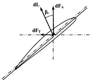
Figure 10 below shows a propeller blade section with the associated inflow velocities and lift force. By definition the lift force, dL, is always perpendicular to the total inflow velocity V*. dL

is responsible for both thrust and torque on the propeller blades and propeller shaft.

Ua

dL t

f'

coR+ut*+VT

(P

Figure 10: Blade Section with Lift and Flow Velocity Vectors

Note that dL is always perpendicular to V* but it is typically not perpendicular to the chord line. Therefore, when determining the component of dL that produces thrust and the component of the

dL which produces torque, the inflow angle

pi

is required, not the blade pitch angle, (pP. The

elemental lift at a blade section is given by Equation 1. 1

dL=-p(V*)2 _{CLcdr (1)}

2 where

dL = elemental lift on a blade section

p =fluid density

CL = section lift coefficient at radius r, this comes from the lifting line calculation in OpenProp.

c = section chord length at r dr = elemental radial span

(22)

dL

Figure 11: Blade Section Showing Lift Resolved into Axial and Tangential Components

From Figure 11, it can be seen that the axial force, FA, and tangential force, FT, at a blade section are given by:

dFA dL cos(,+ ) (2)

dFT =dL sin(,i +c) (3) where

= inflow angle

E CD/CL, inflow angle correction due to viscous effects

CD = section drag coefficient

Note that in Figure 11, the point of application of dL has been shifted to the centroid of the section and is no longer located at the same point as in Figure 10. This is done to simplify calculations. dL will not necessarily be located at the section centroid but at a point approximately % of the distance from the leading edge to trailing edge on the chord line as shown in Figure 10. The fact that dL does not act through the section centroid means that dL will produce a torque about the span line of the blade. This torque and its associated sheer stress are assumed to be negligible along with all other shear stresses.

Both FA and FT produce bending moments about the centroidal axes. Each of these bending moments, along with their x and y components, is shown in Figure 12. The equations for the bending moment are:

dMA =(r-r,)dFA (4)

dMT =(r-r,)dF (5)

where

ro= section radius where dM is being calculated r = radius of section producing lift

(23)

dMA

Ve dMTT

dMT

Figure 12: Bending Moments Components The total moments produced by FA and FT, at a section ro, are given by:

MA = p(V*)2 CLc cos(,+ e)(r-r,)dr (6) ro

MT = ip(V*)2 CL c sin(p, +e)(r -r)dr (7) ro

Because it is necessary to project these bending moments onto the centroidal axes of the section, blade pitch angle is required. Projecting the total bending moments onto the centroidal axes, the equations become

MX =MA cos((OP)+Mr sin(p,) (8)

my

=MA sin(p,) -MT cos(p) (9) (PP

(24)

Each of these bending moment vectors is shown in Figure 13.

Xo

YO

MX

Figure 13: Total Bending Moments about Centroidal Axes

Additionally, the centrifugal force acting at each section contributes to the overall stress at the section. The elemental centrifugal force acting on a blade from an adjoining section is given by

dFc= (2xn)2 _rdm ₍₁₀₎

where

dm = pAdr = mass of blade element Pb propeller blade material density A = section area

c = section chord length t = section thickness

Summing the contributions of all adjoining sections to the Fc at the section of interest, the total

Fc at the section becomes

R

Fc=(2zn)2pb Ardr (11)

r.

Since the blades analyzed using the above method do not contain rake or skew, which would introduce additional bending moments from Fc, the equation for the stress on a blade section can be expressed as:

-MX"y _MY_x _Fc

_-= _- "+ (12)

(25)

Implementation

The following paragraphs are an explanation of the method used to calculate blade stresses. The calculations were performed on a propeller which was designed by Epps (201 Oa) and is shown in Figure 14.

Figure 14: Example Propeller Courtesy ofEpps

In order to implement the equations above it is necessary to calculate the required blade section quantities. Figure 15 and Figure 17 illustrate the overall procedure for determining 2D blade section area, centroid and moments of inertia.

X (M)

Figure 15: Distorted Root Section

Figure 15 shows the visually distorted root section of the propeller shown in Figure 14. The section is distorted for illustrative purposes; the undistorted root section is shown in Figure 16.

Root Section Ordinates 0.01-Upper Surface 0.008 Lower 0.006 Surfac 0.004- 0.002-0 0 0.01 0.02 0.03 0.04 0.05 0.06 e

(26)

OpenProp treats the blade section as an upper and lower surface. The overall procedure for determining blade section area properties consisted of determining the area properties of the area formed by the upper surface and the x-axis and subtracting the area properties formed by the lower surface and the x-axis. This subtraction results in the properties of the enclosed area shown above.

Root Section Ordinates 0.025- 0.02- 0.0150.01 0.005 0.005 0.01 --0.015 1-0 0.01 0.02 0.03 0.04 0.05 X (in)

Figure 16: Undistorted Root Section

Figure 17: Calculation of Elemental Area Properties

(27)

Figure 17 shows a characteristic diagram that was used to determine elemental area properties which were summed to achieve the section area properties. The procedure was:

1. Determine elemental area 2. Calculate elemental centroid

3. Calculate elemental ₂_{"d moment of area about both x and y axes} 4. Sum elemental areas

5. Sum 2nd moment of areas about x and y axes

6. Calculate section centroid, Equation 13

i Ai -- I Al.

Y = ,: X = ( 1 3 )

7. Apply parallel axis theorem to determine ₂nd _{moment of area about the centroidal axes,}

Equation 14.

'Centroid X X Y 2 Atotal Centroid Y Y 2 Atotal (14)

In order to determine the other quantities required by Equation 12, the integrals were turned into discrete sums and variables from the propeller design were used.

Results

The results of the analysis performed for the propeller described in Epps (201 0a) are shown below for an on-design and off-design condition. Figure 18 shows the stress at the blade root. As expected, the blade is in tension on the pressure side and compression on the suction side. Note that the stresses indicated in Figure 18 in the middle of the root section are interpolated stress. Only the stresses at the blade surface were calculated at the points indicated.

0.03

0.02

0.01

-0.01

-0.02

Root Section Stress

Suction Side x10 I 0.5 0 -0 .5 -1 -1.5 ffi--- - - -- P r( 0.04 0.05 0 0.01 0.02 0.03 X (M) essure Side

Figure 18: On-design Root Section Stress

... ... ... .... .... . .. ...

(28)

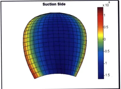
In Figure 19 through Figure 22 tensile stresses are considered positive and compressive stresses negative. Figure 19 and Figure 20 represent the on-design condition while Figure 21 and Figure

22 represent an off-design condition as specified in the figure titles. As expected, the off-design condition chosen shows higher stresses than the on-design condition because the off-design condition corresponds to a point where the propeller is producing greater thrust and torque. Greater thrust and torque results in higher stress.

Fs

Figure 19: On-design Suction Side Stress: J,=O. 75, Vs=1.5m/s, n=;8rev/s, D=0.25m

Figure 20: On-design Pressure Side

Suction Side xlO_{x 10}

S1

0.5

.

J,=6. 75, Vs=1. 5m/s, n=8revs,

(29)

Suction Side

Figure 21: Off-design Suction Side Stress:

7 0.8 0.6 0.4 0.2 0 -0.2 -0.4 0.6 -0.8 -1 J,=0.40, Vs=1.5m/s, n=15rev/s, J Pressure Side _x)10 0.8 0.6 04 0.2 0 )=0.25m

Figure 22: Off-design Pressure Side Stress: J,=0.40, Vs=1.5m/s, n=15rev/s, D=0.25m

Carlton (2007) presents isostress contour lines taken from Finite Element Analysis (FEA) results for various propeller types. The results presented above agree with the trends presented by Carlton for a propeller blade without skew. Carlton shows highest stress near the blade mid-chord in a region that extends close to the tip of the blade and a decreasing stress as one moves away from the mid-chord to the blade leading and trailing edges.

(30)

Limitations

There are several assumptions and simplifications that are made in the method discussed above. Each of these is listed below with suggestions to improve the calculation.

1. Blade Section - In propeller design it is customary to present the blade section geometry as the unwrapped section. In other words, the blade section geometry is the geometry one would obtain if the curved blade section were laid flat. This geometry was used in the calculation of the blade section properties. It is more desirable to calculate the blade section properties for blade sections that were taken using a flat cutting plane oriented perpendicular to the span line. The implementation of stress calculations would be more difficult for a truly flat blade section since OpenProp does not develop the blade

geometry for this type of section nor is the hydrodynamic data valid for a blade section obtained in this way. The OpenProp geometry code could be rewritten to perform an interpolation in order to obtain the points to create a truly flat blade section but the problem of obtaining blade section loading remains. Blade loading could possibly be

obtained using the cavitation analysis module pressures however the stress code would then need to be altered to be something similar to FEA.

2. Geometric Property Calculation - The method used to calculate blade section properties was essentially a trapezoid rule integration. This method was used because it does not limit the selection of the number of points used to design the blade, however other more precise methods could be used.

3. Point of Load Application - In the method presented, the section lift force is applied to the section centroid. This simplifies the code because the actual point of application does not have to be determined and the resulting torsional loads can be ignored. The actual point of lift force application could be approximated as the /4 chord point or could be

calculted more precisely by analyzing the pressure distribution from the cavitation

analysis module. If the load point is corrected, the resulting torsional sheer stresses could be calculated. This correction is probably small for blades without skew.

4. Sheer Stresses - All sheer stresses on the blade section are ignored. The stresses calculated above represent bending stress from lift and axial stress from the centrifugal force. Sheer stress could be included if the load point is corrected and the resulting torsional stress is calculated and added to the sheer stress resulting from the pressure differential between the blade faces. If sheer stresses are included, the principal stresses should be calculated.

(31)

Chapter 6 - Fatigue Analysis

By definition fatigue failure is characterized by a time varying load whose magnitude is smaller than that required to produce failure in a single application, Pook (2007). The fatigue analysis conducted as part of this project is presented in two steps.

1. Identification of the cyclic loading 2. Application of a fatigue failure theory.

A comprehensive fatigue analysis is characterized by many subtleties and in many cases

significant experience is necessary to conduct the art of a fatigue analysis. The fatigue analysis presented here is intended to provide a method by which a fatigue analysis could be conducted on a propeller or turbine at the beginning of the design process to ensure the estimated fatigue life meets the design goal. As a whole, OpenProp is intended to be a design tool which can be used to provide good initial propeller and turbine designs. As additional iterations of the design process are completed more sophisticated tools for propeller design will become necessary. It is

in this spirit of providing good initial design estimates that the fatigue analysis is presented here.

Cyclic Load

For a propeller or turbine the source of the varying load is the wake that it operates in. Due to the presence of a wake, the inflow velocities to the blades are not uniform in magnitude or

direction. As a blade completes a revolution it will pass through regions of various velocity which will induce varying forces on the blade. A propeller will typically operate in a wake with greater inflow velocity variation than a turbine. Because a propeller operates in a more severe wake environment and because wake data is more readily available for propellers than for turbines, fatigue analysis for a propeller was performed.

A wake for a single screw ship is shown in Figure 23. This wake is also shown in Laskos (2010) and was measured by Koronowicz, Chaja and Szantyr (2005). This figure clearly shows a circumferential variation in the axial inflow velocity. Typically there is also a circumferential variation in the tangential inflow velocity but this variation is much smaller and is not considered here. This is shown in wake profiles of Felli and Felice (2005). Figure 23 shows the ship wake divided into twelve sectors. As the blade passes through each sector it is assumed to fully develop lift commensurate with the flow velocity in that sector. This assumption makes this analysis a quasi-steady analysis. In each sector, the circumferential average of the axial inflow velocities was taken at the same radial positions that were used in the propeller design. Each blade section is subjected to a different inflow velocity which results in a different CL. In order to determine the new CL on each section Equation 15 was used.

CL=CLo=+ 2z(Aa) (15)

where

CLo original lift coefficient in the design condition

CLf new lift coefficient at the new angle of attack

(32)

330 ₃₀ _-0.9 300 ,, 60 0.8 10 2 0. 270 9 -- 3 90 0.6 8 4 240 's120 0.5 7 '6 -'5 210 150 0.4 180

V/V

Figure 23: Sectored, Single Screw Ship Wake

Figure 24 and Figure 25 show how a change in the axial velocity produces a change in the magnitude and direction of the total inflow velocity. The analysis also assumes that u*a and u*, remain constant.

oR+ut'

mR+ut~+VT

Figure 24: Original Inflow Velocities

...

(33)

. ... *Ketmlet 10 . Gdc IfMfdW 7 x 10 2 2 3 3 UsbrI~,ev2 to 3iwarmg8 10 22 33 2 2 44 ft"-- 4 104$6w wIwft 3 2 k 0~l s10 as1 2 2

(34)

Figure 26 above shows the change in blade stress as the blade passes through the wake sectors of Figure 23. As expected, the highest stresses occur in sector number twelve where the axial inflow velocity is the lowest. The lowest axial inflow produces the largest angle of attack and lift coefficient and subjects the blade to the largest amounts of lift and stress.

Since the blade stress varies considerably across the blade faces, it is necessary to identify the point where maximum tensile stress occurs. The point of maximum stress for this propeller occurs at the blade root at the point identified by the arrow in Figure 27.

Figure 27: Point of Maximum Tensile Stress

In Figure 28, plots of the maximum blade stress versus angular blade position for various ship speeds are shown. These plots also identify the alternating stress, Ua, associated with each blade

stress. Except for the highest ship speeds, c-a is relatively low, near the endurance limit for nickel,

aluminum bronze, as shown in Figure 29.

(35)

V, -6kts 9 7 -6 - 4M~a A ... l. .. . .. .. . .---.---- . . . .. . . 50 100 160 200 260 300 360

Blade Position (dog)

V,- 10kts 36 26 - ---... --- - .. ..-.-..-.-..-.-26 * -15MPa 10 --- - - - - -* U 5 - - ~ -U -* 0 60 100 160 200 260 30 360

V, -16kts 60 40 -- -34MPa 30 - ---* m 10 - -U -a 60 100 160 200 260 300

360 12 C 0 E6 E 4 W2C 0 C E 6 26 2C 16 2 V - 20kts 0 0 - 7Pa-0L --- - - 0-60 100 160 200 260 300 360

V. - 26kts

0

10M~

60 100 160 200 260 300 360

V, - 30kts

-145MPa

.. . .--- .. ...- - -. . -. .. --. - -.. ... . .

0

60 100 150 200 250

300 360

Figure 28: Maximum Blade Stress versus Angular Position for Various Ship Speeds Using the On-Design

Advance Coefficient (J,=O. 75)

2-7

E 2E E E

(36)

Fatigue Failure

Figure 29 shows a plot of ua, versus number of reversals/cycles to failure for nickel, aluminum bronze. Data for this figure was taken from Kerwin and Hadler (2010); detailed alloy

composition and test condition are unknown. Ideally, one would design a propeller such that blade stresses were minimized in order to increase the fatigue life of the propeller.

Nickel, Aluminum Bronze Fatigue Data

350 300 250 -0.. 150 ...---... 100 'U 10 10 10 10 10 Reversals

Figure 29: S-N Curve for NiAl Bronze

When performing a propeller fatigue analysis it is critical that the operational profile of the ship is taken into consideration. Figure 30 shows an operational profile for a warship which was taken from Gooding (2009). Since the propeller analyzed here was not analyzed for such a wide spectrum of speeds, Figure 31 was used in the example calculation.

Speed (kts)

Figure 30: Operational Profile for DDG51 DDG51 Operational Profile

(37)

Example Operational Profile 30 25 ----20 E 015 5 10 15 25. . U 0 ... . ... 0 5 10 15 20 25 30 35 Speed (kts)

Figure 31: Example Operational Profile Used for Calculations

With the assumptions made in this analysis, there is a direct correlation between ship speed and blade stress. This correlation was used to produce Figure 32 below.

aa (MPa)

Figure 32: Time at Various Stress Levels

Miner's rule was used to predict the fatigue life of the propeller. Miner's rule is simply stated in Equation 16.

r

R- (16)

where

r, = actual number of reversals at o-a

(38)

In order to predict the fatigue life, additional equations are necessary. These are shown below.

RPMI t, (17) where

ti= time spent at rotation rate, RPM,

RPM= rotation rate which produces desired speed

t, =x, T (18) where

xt = fraction of total time spent at RPM

T= total time of propeller operation

Substituting Equation 17 and Equation 18 into Equation 16 and solving for T, one obtains:

T = (19)

RPM, x1

R,

If one considers the blade stress at speeds below 25kts to be of infinite life then the fatigue life is 180 days. This calculation is dominated by the time spent at 30kts which is probably excessive when comparing Figure 31 and Figure 30.

(39)

Limitations

In addition to the limitations discussed at the end of Chapter 5, there are some additional

limitations that are specific to the fatigue analysis. While the method presented here is useful to obtain an initial estimate of fatigue life there are many more factors which should be considered as the intial estimate is refined.

1. Fatigue Data - Figure 29 shows notional fatigue data for a Ni-Al Bronze. It is unknown how this data was obtained and to what specific alloy it applies. It would be desirable to use data obtained in a seawater environment for the specific alloy one intended to use to manufacture a propeller.

2. Miner's Rule Coefficient - In the method above, it was assumed that when the sum of Equation 16 reached unity that the material would fail. This is a reasonable assumption but other's have found that the coefficient should be a number other than one depending on the specific material type (Sines and Waisman 1959). Determination of a more accurate value for this coefficient would involve an extensive test program that should be performed for more refined calculations.

3. Shaft Reversals - Shaft reversals are a routine operation in ship maneuvering, particularly when the ship is near a pier, in high traffic areas or navigating waters that restrict its turning ability. Kerwin and Hadler (2010) and Carlton (2007) provide a limited

discussion on the effect of shaft reversals on blade fatigue life. A shaft reversal can be a highly stressing event for the propeller blade and therefore can significantly reduce the blade fatigue life. Calculating the blade loads during a shaft reversal would require unsteady analysis and is beyond the scope of this project and the current capabilities of

OpenProp.

4. Blade Response - The analysis presented here assumes that the blade will completely respond to the flow regime of each sector. It is unlikely that this is the case. The analysis does not take into account the time element necessary for the blade to fully develop its thrust and in this regard is a conservative estimate of fatigue life.

(40)

Chapter 7 - Test Fixture Design and Construction

This chapter describes the design and construction of a test fixture for testing propellers and turbines. The test fixture described in this chapter was specifically designed for use in the hydrodynamics laboratory water tunnel at MIT but can also be used in a tow tank. The limitations of the test fixture are given in the Table 4.

Limits

Value

Basis

Torque 6 ft-lbf Sensor limitation

Thrust 50 lbf Sensor limitation

RPM 1500 rpm Peak capability of motor

Current 18 amps Peak capability of motor

Voltage 240 V-AC Required supply voltage

300 V-DC Maximum controller output voltage

Table 4: Test Fixture Limitations

The design philosophy employed for this test fixture, with accompanying justification is given below.

1. Thrust and torque sensor must be the limiting component. The sensor used in this test fixture is on loan to Professor Richard Kimball from the US Navy. Searches for a commercially available sensor capable of simultaneous thrust and torque measurement did not yield any devices that could have been used in a test fixture of this size. Because of the limited availability of useable sensors, it was decided that the test fixture should be limited only by the sensor.

2. Components must be usable in other test fixtures. Since there were no other test fixtures of this type at MIT, this design constraint meant that the test fixture must be able to be disassembled and the components able to be used in other test fixture assemblies that might be designed by students in the future. This constraint was a significant driver in the selection of electrical components, manufacture of mechanical components and method of component assembly.

3. Fixture must be able to incorporate a high resolution encoder. This constraint effected the motor and encoder selection process.

4. Fixture must be capable of use in both a tow tank and water tunnel. This constraint drives the maximum allowable overall diameter, length and standpipe length of the test fixture.

Additional details concerning how the design philosophy impacted test fixture design as well as the final test fixture configuration are given in the sections that follow.

MECHANICAL

Thrust/Torque Sensor

The thrust/torque sensor used in this test fixture is a strain gage type sensor. The sensor uses two sets of strain gages; one set to measure thrust and the other set to measure torque. The strain gages are adhered to the center ring shown in Figure 34, which is covered in an opaque epoxy like material. The presence of this material introduced measurement error when building the

(41)

CAD sensor model that was created and is one of the reasons why a factor of safety (FOS) of 2 was used when determining the maximum operational torque that could be applied to the sensor. Since the sensor was to be the limiting component, it was necessary to characterize the thrust and torque capabilities of the sensor. In order to determine the maximum thrust and torque that the sensor could measure without damage, a determination of sensor material was made and FEA of the sensor was performed. For the purposes of this test fixture design, "damage" is defined as a load condition which would produce yielding in the sensor material. FEA required that a three dimensional model of the sensor be made, this model is shown in Figure 33.

Figure 33: Provided Sensor

While measuring the sensor to determine physical dimensions for incorporation into the model, an inscription of 501bf was found on one end of the sensor. 501bf was used as the thrust load on the sensor in the FEA analysis in order to determine a FOS. The result of the FEA showed that the sensor can withstand a 501bf axial load with a FOS of 2. The calculated stress distribution resulting from a 501bf load is shown in Figure 34.

Figure 34: Stress from Axial Load on Sensor (501bf applied)

(42)

The results of the FEA show interference between the center ring of the sensor and the end of the sensor. This interference is a result of the large scale factor necessary to make the sensor

deflections visible and does not represent actual interference when the sensor is under a 501bf thrust load.

In order to determine the maximum torque that the sensor could carry, a separate FEA was conducted. The results of this analysis show that the sensor could carry 12ft-lbf without damage. Application of a FOS of 2, that was determined from the thrust FEA, limited the maximum torque of the sensor to 6ft-lbf. A FOS of 2 is reasonable due to the dimensional error present in the model and a lack of validation of the FEA used on the model of the sensor. A picture of the stress distribution resulting from a 12ft-lbf applied torque is shown in Figure 35. Note that the "handle" that is present in the picture was necessary to apply a torque load in SolidWorks@ 2007 Education Edition.

"Handle"

Figure 35: Stress from Torque Load on Sensor (12ft-lbf applied)

Output Shaft Configuration

Three options were considered for the configuration of the output shaft to which a propeller or turbine could be attached for testing.

1. A tapered shaft capable of accepting the fittings already manufactured and located in the water tunnel laboratory.

2. A straight shaft with a pin, similar to that used for propeller attachment to trolling motors. 3. A straight shaft with a flat side machined.

Option 1 was undesirable because the shaft size required to accommodate the taper would have required larger bearings and seals for the shaft which would have increased the friction resistance on the shaft and made sealing the shaft more difficult. Additionally, a larger diameter shaft has greater rotational inertia which would limit the rate at which the shaft could be accelerated during unsteady tests.

(43)

Option 3 was less desirable than Option 2 because of the complication of manufacturing propellers with a set screw hole. The intended manufacturing technique for propellers is 3D printing. Propellers manufactured using this method are made from ABS plastic. Successfully creating a threaded hole into this material with sufficient holding power for a set screw seemed unlikely. A second problem with this type of shaft is that it required a female section to be made in the propeller hub that would have been difficult to machine: a straight cylindrical hole that changes to a cylindrical hole with a flat. Previous experience manufacturing propellers using the 3D printing technique has shown that it is difficult to achieve a hub whose outer diameter is concentric to the drive shaft hole outer diameter. Therefore it is necessary to turn the propeller on a lathe to ensure that the drive shaft will easily attach to the propeller with minimal

eccentricity between the inner and outer diameter of the propeller hub.

Option 2 requires that every propeller have a slot machined in the hub but this operation is simple using an end mill of the same size as the output shaft pin. It is also possible to print the slot in the hub if the turbine is manufactured using a rapid prototyping technique. Option 2 also requires that the end of the drive shaft be threaded to accept a nut to hold the propeller against the drive shaft pin, however these are external threads that are easy to manufacture. For these reasons, Option 2 for drive shaft configuration was chosen. A picture of the shaft is given Figure 36.

Figure 36: Output Shaft Configuration

Drive Shaft Configuration

The test fixture design described in this paper is intended to be used to test both propellers and turbines. Because of this dual use capability, it is necessary that the fixture be able to measure and support axial loads in two directions. Including the capability to support axial loads in two directions also protects the fixture from inadvertent damage should a load be applied in an axial direction for which the fixture was not designed.