Design, development, and characterization of an experimental device to test torsion-controlled fracture of thin brittle rods

Design, Development, and Characterization of an Experimental Device to Test

Torsion-Controlled Fracture of Thin Brittle Rods

by

Ronald Henry Heisser

SUBMITTED TO THE DEPARTMENT OF MECHANICAL ENGINEERING IN PARTIAL

FULFILLMENT OF THE REQUIREMENTS FOR THE DEGREE OF

BACHELOR OF SCIENCE IN MECHANICAL ENGINEERING

AT THE

MASSACHUSETTS INSTITUTE OF TECHNOLOGY

JUNE 2016

2016 Ronald Henry Heisser. All rights reserved.

The author hereby grants to MIT permission to reproduce and to distribute publicly paper and

electronic copies of this thesis document in whole or in part in any medium now known or

hereafter created.

Signature of Author:

Certified by:

Signature redacted

Department of Mechanical Engineering

Signature redacted

J5rn Dunkel

Assistant Professor of Mathematics

Signature

JUL

0 8

2016

LIBRARIES

Thesis Supervisor

Anette Hosoi

Associate Professor of Mechanical Engineering

Undergraduate Officer

Design, Development, and Characterization of an Experimental Device to Test

Torsion-Controlled Fracture of Thin Brittle Rods

by

Ronald Henry Heisser

Submitted to the Department of Mechanical Engineering on May 6, 2016 in Partial Fulfillment

of the Requirements for the Degree of Bachelor of Science in Mechanical Engineering

ABSTRACT:

As research continues to uncover the many different physical properties of meso- and microscale materials, it becomes more evident that these materials often behave in counterintuitive ways.

Characterizing unique phenomena not only provides analogies in nature which inspire innovation at all levels of research and design but also presents new possibilities for future technological development. The discussion presented herein explores the design and development of a low-cost, manual device intended to test a hypothesis rooted in the behavior of breaking pasta that intrigued even Richard Feynman. While the mechanism for why spaghetti breaks into three or more pieces has been described, the experimental discussion presented here focuses on the effect that added torsion has on the fracture bent spaghetti. Specifically, it is possible that twisting the spaghetti a critical angle and bending it will cause it to fracture into only one piece. The idea of torsion being used to exhibit some control over how a material fractures has not been well-investigated; the results which come from this experiment may prove useful for applications even beyond the scope of thin brittle materials. With this said, the sensitivity in quantifying breaking from torsion and bending together requires that the experimental device prevent systematic error stress from negatively impacting the accuracy of the experiment. Thus much time is devoted to explanation and rationale behind the analysis of the experimental device. Alongside the device's characterization this thesis serves to be a reflection of the design process taken while creating this device. Lessons learned from this project are included in all aspects of the discussion and a section in the Appendix is devoted to a more detailed account of the design and fabrication of one device

component.

Thesis Supervisor: J6rn Dunkel

Acknowledgements:

The author would like to recognize those who helped by advising, educating, and encouraging him with respect to the various aspects of this project. First and foremost the author would like to thank Professor Dunkel for taking a small risk by providing the author the opportunity to independently pursue a small scientific idea and holding him to a high standard; the learning experience has been meaningful enough but hopefully the data which comes at the end will make the effort worth it. Thanks to CADLAB and MakerWorks for providing rapid prototyping resources and on-demand assistance with fabrication techniques. The author is also indebted to the MIT Hobby Shop and the Edgerton Student Shop for assistance in design and manufacture of the very tedious "spaghetti collet", another substantial learning experience. Thanks should also be given to Professor Slocum for allowing incorporation of this thesis work into the author's 2.70 project, and to members of the Spring 2016 2.70 class for the great idea of gripping samples using adhesives. Last but not least the author would like to thank Dr. Norbert Stoop for his interest in the project and his eagerness to help with various mechanics questions which come his way.

Table of Contents

List of Figures and Tables

6

1 Definition of Terms

8

2 Introduction and Motivation

8

2.1 Note on Original Research

8

2.2 Discussion of Results from Class Project

10

3 Design Goals and Functional Requirements

12

3.1 Outline of Functional Requirements

12

3.2 Design Strategy Planning

13

4 Design Strategy

14

4.1 Early Design Scope

14

4.2 Strategy Selection Process

15

4.3 Degrees of Freedom

18

5

System Component Selection

19

5.1 Linear Motion Stage

19

5.2 Torsion-Controller

20

5.3 Component Costs

20

5.4 Fabrication Methods

21

6 Stress Characterization

22

6.1 System Analysis Outline

22

6.2 Linear Misalignment

23

6.3 Angular Misalignment

25

6.5 Sample Constraint Error

28

6.6 Pivot Friction Error

28

6.7 Set Screw Sleeve Holding Torque

30

7 Device Measurements and Error Propagation

32

7.1 Description of Measurement Method

32

7.2 Linear and Angular Error of Pivot Axis

32

7.3 POI Position and Angular Error

33

8 Future Considerations

34

8.1 Device Improvements

34

8.2 General Applications

38

8.3 Further Research in Fracture Control

39

Bibliography

40

Appendix

41

Appendix A: Design Process: Creating a Spaghetti Gripper

41

List of Figures and Tables

Figure 1: A&N experimental diagram

9

Figure 2: Euler-Bernoulli model diagram

9

Figure 3: Diagram of average curvatures for initial fracture

11

Figure 4: Proposed device kinematic diagram

11

Figure 5: Pivot frictional error diagram

13

Figure 6: Example brainstorm drawing

14

Figure

7:

Torsional-controller mounting diagram

16

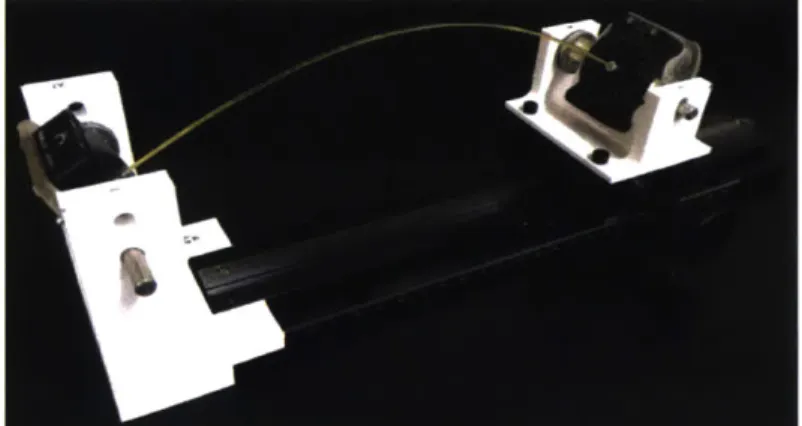
Figure 8: Image of final experimental device

19

Table 1: Bill of materials

22

Figure 9: Shaft misalignment diagram

24

Figure 10: Angular misalignment diagram

26

Figure 11: Intrinsic straightness error diagram

28

Figure 12: Shaft friction diagram

29

Figure 13: Coordinate measurement system diagram

32

Table 2: Calculated parameters from stress characterization

34

Figure 14: Image of final device displaying underside of pivots

35

Figure 15: Image showing 3D printing results

36

Figure 16: Cost vs performance diagram

37

Figure 17: Compact direct-drive motor mount

37

Figure 18: Top-view image of final experimental device

38

Figure 19: First iteration spaghetti grippers

41

Figure 20: Diagram of second iteration spaghetti grippers

42

Figure 21: Image of spaghetti gripper on moving pivot post

43

Figure 22: Image of third-iteration gripper with broken spaghetti

44

Figure 23: Image of first successfully fabricated spaghetti collet

45

Figure 24: Image of CNC lathe cutting operation

45

Figure 25: Lathe machine interface

46

Figure 26: Results after improper use of slitting saw

47

Image

1 Definition of Terms

It will help to make clear terms which are used for rotation since there are two distinct rotations

of interest: the rotation of the pivot and the angular deformation of the sample about its longitudinal axis.

"Pivot" and "moment" all refer to those rotations the two pivots of the experimental device, A and B in

Figure 3, undergo during experimentation. "Angle of deflection", "torsion", and "twist" all refer to the

angular deformation of each sample about its longitudinal axis, C in Figure 3. Here, "longitudinal axis"

means the line which goes along the length of the spaghetti through the center of its cross-sectional area.

Elsewhere, "deflection" refers to the linear deformation of a beam or shaft from equilibrium straightness.

Additionally, "angle" will be used in describing both rotations. Different symbols for angles are given for

depictions of figures and variables in equations but will be defined each time before they are used.

2 Introduction and Motivation

Although the device described in this discussion can function for tests of a vast array of materials,

the original intention is to test the effect of combined torsion and bending on the post-fracture dynamics

of raw spaghetti strands. It has long been observed that raw spaghetti, when bent in half, would almost

always fracture into three or more pieces. This non-intuitive phenomena has historically puzzled many,

even notable scientists such as Richard Feynman (Sykes p. 180-181).

2.1 Note on Original Research

No satisfactory explanation of why spaghetti exhibited this behavior was given until 2005 when

Basile Audoly and Sebastien Neukirch (A&N) co-authored a paper titled "Fragmentation of rods by

cascading cracks: why spaghetti do not break in half' (A&N p. 1). In this publication the authors show

that the mechanism responsible for this behavior is a series of progressive flexural waves which travel

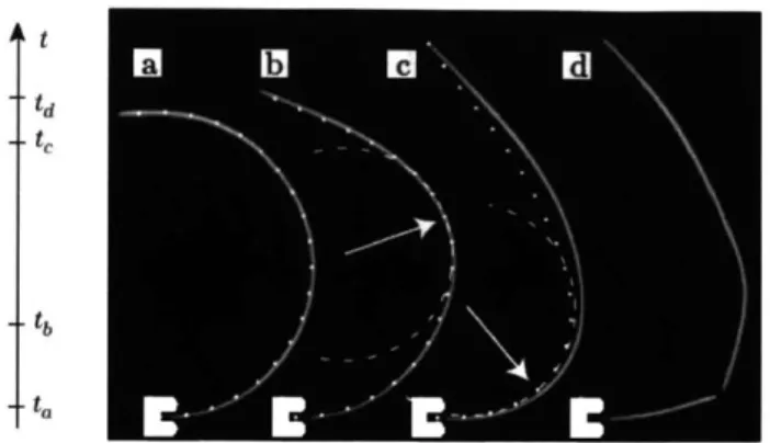
Figure 1: A&N experimental diagram. Images taken at different times after free spaghetti end is released (A&N p. 3). It is important to note the differences between this experimental setup and the one described in this discussion. Here, the experiment simulates the dynamics after a spaghetti has already broken once. The ends of the spaghetti are then modeled as rigid supports, as seen at the bottom of this figure. The dotted lines represent the analytical solution they give in their paper and the dashed line represents the osculating circle as the flexural wave travels down the spaghetti axis; the arrow specifies the approximate radius of curvature at the point of interest.

As the spaghetti is bent, the curvature grows and thus the stored energy is also increased. Where local curvature is highest, bending the spaghetti past a critical curvature causes a brittle fracture which results in a stress relaxation down both halves. While the total stress may decrease from energy dissipation the speed of the flexural waves actually cause a local increase in curvature along the spaghetti's length, such that at one or more points the curvature may increase again to a critical level, resulting in additional

fractures (A&N p. 2).

L

Figure 2: Euler-Bernoulli mechanical model diagram. Represents analytical model A&N use in their own theory and experimentation, taken from publication (A&N p. 1). This experimental setup assumes a symmetrical first fracture thus simulating the post fracture dynamics to capture additional breaking phenomena.

With this said, there is still a possibility that the spaghetti need not always break into three or more pieces; there might be a special deformation for which only one fracture happens. Granted: for strands of raw spaghetti shorter than a certain length, the spaghetti would break only into two pieces if bent in half. One could also take a knife and cut a spaghetti in half. However, these alternatives seem not to capture the spirit of what is considered interesting.

2.2 Discussion of Results from Class Project

As a class project for 18.354: Nonlinear Dynamics: Continuum-Systems, the author and a class

partner sought to determine whether it was possible to prevent additional fractures by only manipulating

the spaghetti in a certain manner. After various methods and attempts were made, it was found that

twisting the spaghetti before bending it often caused it to only break into two pieces. Thus this

method-done by hand-was further explored by conducting a first-order experiment using high speed cameras.

Since the experiment gave some initial support for the validity of this hypothesis, it will help to provide

the mechanical argument behind why twisting the spaghetti before bending it may prevent additional

fractures.

It is easy to test and verify that past a certain local critical curvature K, the spaghetti will fracture

at that point. A&N show that subsequent additional fractures occur when flexural waves released from the

initial fracture locally increase the curvature down the length of the spaghetti enough to bend it to another

local critical curvature K* and break again (A&N p. 1). Since these breaking events depend on the initial

energy released by the flexural waves, it is also true that if the initial curvature at breaking is sufficiently

less than K. then the flexural waves will not produce a local curvature such that it reaches K*. Then the

challenge would be finding a way to break the spaghetti at a curvature lower than K. It is believed that

applying a torsion to the spaghetti in addition to normal bending will accomplish this task because the

stress required to initiate a crack in the pure bending case will be the same as the bending and torsion

case, yet the presence of torsional stress requires a lower bending stress for the same total stress. Using

the von Mises equivalent stress qe, this relation can be shown as

Ue= ob= U o2t + 312, (1)

where Oob is the initial breaking tensile stress in the pure bending case, 0

0t is the initial breaking tensile

stress in the added-torsion case, and r is the shear stress from torsion (Heisser & Gridello p. 7). Finally, r

to the increase in curvature. If this is true, then the spaghetti can break at a lower curvature in the

added-torsion case than in the pure bending case and not involve any further fractures.

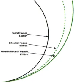
Normal Frackire 6 536cm Bifurcation Fracture 8 700cm Revised Bdurcation Fraclure 9.70Bcm

Figure 3: Diagram of average curvatures for initial fracture (Heisser & Gridello p. 9). The black line represents the curvature of the normal bending case, the green lines represent the added-torsion case. Since only five samples per case were tested and recorded, the curvature including unfavorable measurements was also included. Yet even from a small sample size these results give grounds to believe that the added-torsion hypothesis has some promise.

When initial experiments were done by hand, resulting analysis showed that added-torsion cases did in fact have a lower curvature than a pure bending case. And when unfavorable measurements were

excluded from data analysis, the single-breaking events had an almost 50% lower curvature than the pure

bending events [Figure 3] (Heisser & Gridello p. 10).

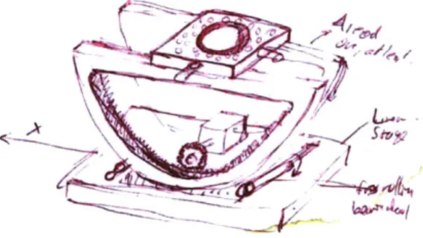
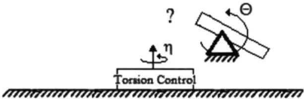
Figure 4: Proposed device kinematic diagram. This diagram taken from final 18.354 report and involves a stationary pivot, linearly translating pivot, and torsional component connected to the translating pivot (Heisser & Gridello p. 10).

However, these results still not reliable enough to make any definitive conclusion since the experiments were done by hand. For a more convincing set of data, an apparatus would have to be designed and

fabricated to ensure that an experiment was sufficiently repeatable. Such a system is described and

characterized in the rest of the discussion.

3 Design Goals and Functional Requirements:

3.1 Outline of Functional Requirements

Once the research question was clearly defined, it was then possible to develop a set of goals to

be achieved in the design process. For the purposes of this discussion, such goals are not directly related

to the results of the experiment but are limited to the realization of a set of design concepts in the device

itself. However, these two goals are of course inextricably linked; device testing and analysis shall give

good credence as to the future success of the device during experimentation.

The functional requirements are listed as follows:

* Allow experimental sample to freely pivot at its two ends

" Provide adjustable applied torsion to experimental sample * Accommodate experimental samples up to 250mm long

" Have sufficient repeatability and measurement accuracy * Feature low cycle time for experimental runs

* Be easily portable

* Fit within a budget of $500

* Have low system complexity and low fabrication time

Note that in these requirements there is no mention of how each requirement will be fulfilled;

choosing a strategy is its own distinct part of the process. Each of these requirements have independent

rationales. The experiment called for a "pure bending moment", or bending just as a function of two ends

being pushed together with no added external moments. The parameter of interest is curvature;

conducting testing without applied moments at the ends would prevent unwanted stress concentrations

within sample and give the simplest post-experimental analysis, increasing the viability of experimental

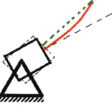
Figure 5: Frictional pivot error diagram. Shaft is loaded by frictional error-induced moment as a result of not properly rotating to eliminate moment. Diagram shows sample constraint as black box with dotted black line the line perpendicular from the box face mounted on pivot (grounded triangle). The red line shows how the sample deflects from its ideal configuration. The dotted box shows the ideal rotation for a given position. and the green dotted line the ideal contour of the sample. For any sliding pivot. there will alvays be some undesirable loading as a result of rotational friction. The design must account for this fact in analysis.

3.2 Design Strategy Planning

A variable applied torsion capability is simply a requirement of the experiment, as one of the main tenets is to find a critical angle at which samples would bifurcate and cause no additional fractures. Precision control of the torsion (and bending) allows for a higher resolution in testing variability which results in more insightful experimental data. The length accommodation is particular to the experiment for which this device was created, though it is assumed that meaningful tests can be done on other materials of similar lengths. In this case, cost constraints limited the materials available for purchase.

Even at this stage, it is of importance to begin visualizing the actual experiment-in-progress as this shall inform certain details in the design which have the potential to significantly hamper the actual experimental process. Especially in small-scale experiments, something like cycle time, if not addressed soon enough. can require a significant change to the design of the experiment. For this discussion, one will see cycle time addressed most directly in the design of the sample-device gripping interface. An in-depth discussion of the gripper design is provided in the Appendix.

The budget constraint is simply a reality of the project. A bill of materials will show the cost of device components and potential capital, machining costs for fabrication, the true total cost terminating in the $500 range. Lastly: low system complexity and fabrication time might seem like a somewhat

ambiguous or unmeasurable design goal, but since this device is to be used for potentially hundreds of runs, it is essential that the design complexity match the complexity of the project. Continually asking

questions like "Is this necessary to achieve the desired function?" and "Will this be hard to fix if broken?"

should also help to point designs in the right direction. Thus, simplicity is not so much a design goal as it

is one of many guiding principles to help make the project successful. Next: a set of potential strategies,

early-stage problems, convergence on a best design are discussed.

4 Design Strategy and Device Concepts

4.1 Early Design Scope

Generally in the design process a certain amount of time is explicitly dedicated to brainstorming

different strategies which fulfill the functional requirements, or design goals, enumerated at the beginning

of a project. In this case, a research question had already been sufficiently defined prior to beginning the

project, and given the constraints of time and cost, many design decisions were made. With regards to the

experiment, it was determined that the most resource efficient method of analysis would be to record the

experiment using a high-speed camera and characterize the stress and fracture phenomena of each sample

from investigating video camera data by numerical methods. From this decision, the need of sensors or

computer-controlled device components was essentially eliminated. Given that the device was sufficiently

repeatable, a camera would account for the intrinsic manual variance of the experiment.

Figure 6: Example brainstorm drawing. Already this sketch hints at possible incorporation of available rotary components. While the mechanism drawn is rather complex for the purposes of this experiment (motor connected to curved rack and pinion), it is often good to get everything out of one's mind at once, then return to rationally choose more simple configurations.

When considering the actual nature of the device, there were four early considerations which

experimental sample, placement of a torsion-control element, choice of precision components, and a satisfactory gripping mechanism.

4.2 Strategy Selection Process

The first consideration is essentially a restatement of a functional requirement of the design.

Since the angle of the ends of each sample at any distance between two ends could be deterministically

defined, it is possible to construct a mechanism which rotates the ends of the sample such that the ends

have no moments applied to them. Yet this requires analysis of any gear components which would be

included in this mechanism, significant manufacturing time, lower portability and higher complexity, and

would increase the cost of the device. Such a solution would have a resolution at the level of the

components used.

If this route were taken, we could consider such a solution to be a position-based solution. In this case what is really controlled is the bending angle of the end of the sample rather than a linear position, as

is usually the type of design for many axial tension testing machines. The other solution available as a

design strategy would be force/stress control (in the case of this experiment control of moments).

Generally this implies that one would set a desired force on a computer which subsequently would be

applied to the experimental sample; usually this strategy would then involve either a complex mechanism

or some computer-controlled components and sensors to accurately apply forces. Since the optimal design

of this particular device minimizes any applied force, any computer strategy would involve setting the

applied moment to zero.

Therefore, there is an opportunity to take advantage of unity in this experiment; the strategy

chosen was to allow the sample itself to control the moment-to minimize its own stresses. Moments at

sample ends could then be minimized by allowing the ends of the sample to freely pivot, resulting in pure

bending. While this design choice may be the simplest out of all options, it should be noted that it also has

its own limitations; the resolution of this design choice is the friction of the pivots and requires sufficient

Since finding a critical angle at which a raw spaghetti strand will break into no more than two

pieces is the main aim of the project, it is simplest (and potentially most cost-effective) to choose a

solution which allows for an angle of torsional deflection to be controlled and known for the experiment.

Therefore, like the choice of using a manual method of sample manipulation, this design decision also

naturally falls out of the research question definition and design constraint. However, an additional

constraint is added given the previous choice of having low-friction pivots. Most generally, the frictional

force is proportional to the normal force: the weight of the component which pivots. Given that the

torsion-controlling component must connect in some way to the sample without changing the axis of

rotation of the pivot, the weight of the torsional component must be factored in with any other

components that make up a pivot.

A design in which the torsion component was attached to the sample through a rigid coupling mechanism was initially considered but since a sample would pivot as the experiment was conducted, a

worry about maintaining the same angle of deflection made this strategy less desirable.

TwOsion _I Control

M? o Irrr

Figure 7: Diagram illustrating potential issues with keeping torsion controlling component separate from pivot interface. The torsion controller would ideally be able to rotate an arbitrary angle q which matches the actual twist angle in the sample. However, given that the pivot is able to freely rotate any angle R. a change in 0 might also change actual twist angle on the sample. Additionally having a cheap and simple connection between the torsion control, pivot and sample is not a trivial consideration.

With this in mind and given the fact that any additional components contribute unwanted complexity to

the design it was decided that the torsion controller should remain on the pivot. Nevertheless, the risk that

friction may cause too high an unwanted moment on the sample is still very present; this risk has now

been shifted to choosing materials and geometries which mitigates this risk.

Choosing precision components is not a design consideration that requires significant

deliberation; these components were to be purchased and not custom designed and fabricated. Here, a

main research question corresponds to fracture phenomena, and so a large part of the experimental

precision will be captured by the high-speed camera used: if the length of the sample is specified, then the geometry of the sample at fracture could be accounted for by the camera and subsequent numerical analysis. With this said, precision components are still chosen to preserve uniformity between different

experiments and to maintain repeatability of unwanted stresses applied to each sample.

Given any specific experimental device, its precision allows good predictions to be made about

the effect of misalignments and motion errors on the stress applied to the sample. As a design constraint,

choices had already been made to have manual precision components; precision must fit within this limitation and the first limitation of budget. It is shown in the next section that these constraints are no

problem for manual precision components and that many possible combinations are available which

satisfy experimental needs.

Quite easily the most tedious, time-intensive and complex part of the strategy phase-and all

phases-of the design of this device, the component which holds each sample and connects it to the rest of the system is crucial to the success of this device. This component has the title of "gripper" or as such a part was originally assumed to grip the sample and hold it through frictional forces (the more general term

"constraint" is also used). The design of this component can be broken down into its own set of requirements:

* Not slip from deflection of torsion-control component

* Contribute minimal unwanted stresses to sample under testing * Have repeatable experimental performance

* Ensure low experimental cycle time

Since there are no common low-cost commercial grippers for thin material samples, this part of the device had to be custom-designed and fabricated. The design of a working gripper involved an amount of time

and thought disproportionate to the rest of the design process, and thus is given its own special treatment

in the Appendix. However, the assumption that a component which held samples in place with respect to

the torsional-controller turns out to be an unnecessary one. In the next section it will be shown that an

4.3 Degrees of Freedom

Before the conclusion of this section, it is good to check the viability of this design as it pertains to the degrees of freedom (DoFs) of this conceptual system, before any components are chosen, ordered, fabricated, and assembled. As this device is completely manual (disregarding use of a high-speed camera), repeatability demands that the system be 1 -DoF. There are two pivots and at least one torsion-control component, as well as a linear motion axis to bring the two ends of the sample together in pure bending.

Starting with the sample in free space, there are six degrees of freedom: motion in the x, y, and z directions, and roll, pitch, and yaw. Constraining both ends to pivoting axes means that all linear and rotational DoFs are constrained except possibly for rotations about the cross-section of a sample. Yet the torsion-controller takes away this DoF, given that it does not freely rotate. Including the ground as a motion constraint, DoF then becomes minus one. But one pivot is free to move linearly along one axis. Additionally, most DoF calculations apply only to one rigid bodies; the sample's compliance in bending brings the system back to one DoF. A more formal way of approaching this question is to use the planar Chebychev-Griibler-Kutzbach criterion, or more simply, the mobility formula for planar motion:

i

M=3(N-1-j)+

fi

i=1

In this case, N = 3 since there are two (assumed) rigid links, the sample and ground, and one slider. There

are three joints, each with one degree of freedom, so

j

also 3. Then M = _{0. If one link (the sample) is considered to be compliant in the bending direction,}

though, then M = 1, the desired system DoF. The same result can be achieved by breaking the single link

representing the sample into two links joined together by a pin.

5

System Component Selection

With a complete strategy it is then possible to move onto component selection and

fabrication/assembly considerations. It was decided that the manual actuator and torsion-controller

components should be procured first since they would drive the rest of the assembly and because the

experiment would rely most heavily on their precision and quality. Therefore these two items took first

priority in the budget.

Figure 8: Image of final experimental device. Path to this assembly outlined in rest of section 5. Page belore introduction includes .exploded" view of assembly.

Choosing an appropriate manual linear actuator ended up not being a trivial task, as the vast

majority of manual precision linear components have a range of travel no greater than 2 inches. Often for

optical applications, these stages serve for fine-tune adjustment of lenses/mirrors, and can often be seen as

slide adjustment mechanisms in many microscopes. This is to be expected, since most linear travel

options are in fact computer controlled. It would be possible to remove all computer numerical controlled

(CNC) components of a linear axis and outfit it to be used as a manual system, but stages that can accommodate sample lengths up to 250mm cost on the order of thousands of dollars. thus putting that

option out of this budget.

Fortunately, a 250mmn manual long-travel linear translation stage was found at the Edmund

Optics website which fulfilled the design criteria necessary: 0. 1 mm resolution (well within the acceptable

range of precision), $250 total cost, for track and carriage, a gib with adjustable preload and a knob for

manually adjusting carriage position. Additionally the manual linear stage had multiple threaded holes

5.2 Selection of Torsion-Controller

After a brief survey of possible components to serve as a torsion-controlling element, it was

decided that a manual rotation stage would best fit the needs of the experiment since one would be able to

then simply set the desired angle of deflection. In this case there were actually a variety of precision

rotation components available for purchase. Like the manual linear stages discussed above, these were

usually intended for optical applications. Given the additional design constraint that this component

would freely pivot and thus should have the smallest weight possible, size was a limiting factor. And

since the maximum angle of deflection was hypothesized (first-order investigation described in

Introduction) to be within one full rotation, a continuous-rotation stage was also preferred. Typically these

"micro" rotation stages cost within the range of $50-$350; Thorlabs sells a manual continuous rotation stage with its own mounting surface weighing less than 0.5lbs and locking mechanism for $70, this was

chosen as the mount of choice.

As a caveat-it was suggested during the design of this system that two stages be purchased to

preserve as much symmetry in the experiment as possible; if there was one, the resistance to rotation

would feature an unsymmetrical rotation of the ends of each sample strand resulting in possible

experimental error and unwanted stress along the sample. Thus, one additional rotation stage was

procured for later assembly.

5.3 Cost of Components

Including shipping costs, the purchase of precision components takes up about $400 out of an

available $500. Given that thoughtful choices were made in allocating such a large majority of the budget

to these components, this is not means for worry about the goodness of the design; some options are less

flexible than others. However: remaining resources must be given more careful consideration prior to

additional purchases, and it may be necessary to take advantage of other available lower-cost options for

design of this device was carried out in an environment which has a large amount of materials, fasteners, and tools available to the community for no cost.

It was decided, then, that the majority of components from here on out would make use of these

free materials. Yet this comes at a cost of its own; what is not purchased must be designed, made, measured and finished in-house. Time and the possible need to learn new design/fabrication techniques

must be considered when taking this minimum cost route. Here, necessity dictates that route and enough

time was available to account for this caveat. In the Appendix one will observe that there is a risk

involved with custom designing when behind on a learning curve and how initial estimations of time

required to complete a task may be off by orders of magnitude.

5.4 Fabrication Methods

As a final point of discussion: structural components to interface all the precision stages, pivots,

and mounts for rotary stages were fabricated using stereolithographic (SLA) and fused deposition

modeling (FDM) 3D printing methods. This fabrication method will be shown to provide satisfactory

compliance for the purposes of the experiment in the error analysis section; additionally, 3D printed

materials are very easily machinable, can go through many iterations, and also provide a naturally

low-friction surface for the pivot axis to freely rotate. In general, one should only use 3D printed materials in

precision devices if absolutely necessary, for these purposes the forces acting on the system and the actual

motion of each component are low enough that the effects from any geometric error or material strength

are negligible. Data is recorded by camera, analyzed by software; the goal of the experimental device is to

constrain each sample in a repeatable manner and to eliminate unwanted stress on the sample to allow for

the desire phenomena to be studied.

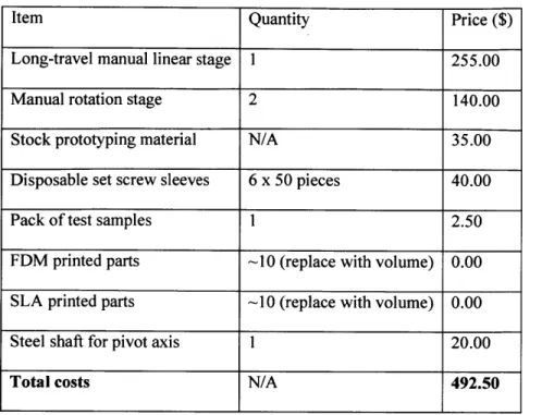
A bill of materials is presented below to capture additional costs associated with the device materials (excludes any purchases for the experiment itself). Some items are not discussed here and will

Item Quantity Price

($)

Long-travel manual linear stage 1 255.00

Manual rotation stage 2 140.00

Stock prototyping material N/A 35.00

Disposable set screw sleeves 6 x 50 pieces 40.00

Pack of test samples 1 2.50

FDM printed parts -10 (replace with volume) 0.00 SLA printed parts -10 (replace with volume) 0.00

Steel shaft for pivot axis 1 20.00

Total costs N/A 492.50

Table 1: Bill of materials. Does not take into account additional costs for running experiment. This given cost does not take into account capital costs and thus assumes that designer has free access to various machine tools, cheap components (such as fasteners) and 3D printers.

6 Stress Characterization

Most experimental machine designs which involve either considerable forces or motion of high enough speed to bring into question component performance involve supporting analysis which

demonstrates that a given system "hits the mark" in desired performance. This mark is one of accuracy, resolution, repeatability, functional life, among other parameters. For the purposes of this device, what needs to be handled is the stress on the samples being tested. The device's original intention is for an investigation of the thin, brittle fracture dynamics of thin rods and requires that the device ensure that the fracture and subsequent dynamics not stem from forces imposed on samples by the device itself.

Therefore, the system must meet a certain stress criteria in order to have the desired performance. Performance can be modeled as how far below a critical allowable stress is placed on each sample. So one can work backwards from the fracture mechanics of each sample (in this case, spaghetti) to the intrinsic motion and alignment errors of the system and how they impart unwanted stress on each

sample. Here, alignment errors are how the effects of limited accuracy in machining and placement of components affect the resting position of a sample. How out-of-plane is the spaghetti before the

experiment begins? Motion errors result from surface imperfections and relative motion between different components. In the subsequent description of analysis one shall see this arise from friction within the system.

Additionally, all assumptions about system performance should, if nothing else, be checked through first-order calculations, as any design choice is liable to bring about significant problems downstream. The more quick analytical considerations are made, the more likely any potential red flags will be addressed early on in the process. And although this section is presented as separate from the design goals, strategy, and component selection phase, a more honest depiction of a proper process would feature this in tandem with the others. This section will feature first a description of the theoretical allowable stress on any given sample, then show actual measured system performance with respect to this allowable stress. Lastly other significant performance calculations will be made to check certain

assumptions.

6.2 Linear Misalignment

For this experiment there are three main forms of unwanted stress which will affect experimental results: linear misalignment, angular misalignment, and pivot angle error. Since the experiment involves a deliberate torsion by twisting each sample a certain angle, deflection error only matters inasmuch as it causes deviation from observed vs. actual angle of deflection. Yet this undesired deflection can be considered a process error and minimized by care in setting up each experimental run. In any case, we can define the total deflection angle V on each sample as:

S= 'Pa + 'Pe (2) where Pa is the applied angle of deflection and Pe the process-induced deflection error. Given that

precision rotation stages are used with 20 arcmin (one-third of a degree) resolution, for deflection angles greater than 10*, Pe is negligible.

Before any derivations, note that the main "mark" by which device performance shall be

measured is the ultimate tensile strength (UTS) of the spaghetti. The Appendix shows results from a first-order experiment used to determine this UTS; the UTS used to base the device analysis is 70MPa. Given a safety factor of 5, _{the maximum allowable stress the device may impose on a given sample is ~14MPal.}

This number will be referenced when actual error values are determined.

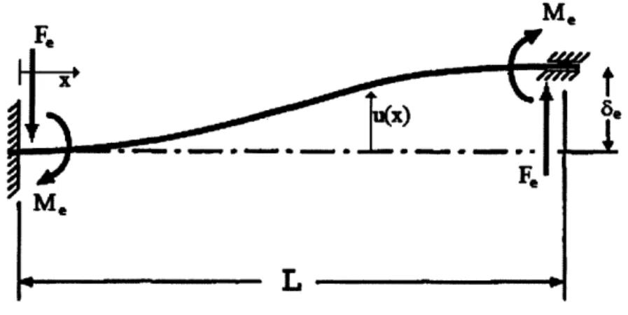
Linear misalignment is taken to be much smaller than the length of each sample. Therefore, forces can be modeled by considering a shaft rigidly supported at both ends with one support displaced a small distance 8e away from the axis of the other support.

Me

x

Me

L

Figure 92: _{Shaft misalignment diagram. Displays shaft reaction forces and moments due to linear misalignment, given that shaft}

is rigidly supported at the ends. L is the length of the shaft. u(x) is the displacement function of the shaft. F, is the reaction force at supported ends, Me is the reaction moment at the supported ends, and 6, is the deflection at the end of the shaft, u(x = L).

Assuming that the shaft's equilibrium state is to remain completely un-deformed and perfectly straight, this displacement results in reaction moments and forces applied to each end of the shaft. Since there are no externally applied forces on the shaft, taking the sum of moments gives the relation

SIt _{is important to note that after first fracture, system and process errors which impose unwanted stress on the}

experimental sample are assumed to vanish given the elimination of kinematic constraint which comes with facture. Thus the only system characteristics which can contribute unwanted stress to the sample are the rotational inertia of the pivot itself and the stress added by the gripping component. In the final iteration adhesives contribute no stresses to samples. The impact of rotational inertia of the pivot is not considered in this discussion and could be interesting

to investigate for future system analysis.

2 Adapted from figure found at

https://www.osapublishing.org/ao/fulltext.cfm?uri=ao-33-19-4109&id=42037#articleFigures. Other figures above and below made by author and may use parts of this original figure for uniformity

M9 = 0 = 2Me - FeL, (3)

where Me is the error moment, Fe is the error force (Winter p. 30). Then,

Me

2

Since only Se is given for this model, Fe must then be related to 6e. Given that the shear force V(x) along the length of the shaft is simply -Fe, the moment M(x) is

M(x) = -Fex + Me. (5)

With this, the deflection u(x) can be evaluated. Given that

a2

u M(x) (6)

ax2 =E(x)I(x)'

where E(x) is Young's Modulus of the shaft and does not vary along x and I(x) is the area moment of inertia (also constant for all x). Integrating twice results in the expression

U() = Fex3 - Mex2 + C1X + C2

C1 and C2 being constants of integration. Given boundary conditions (for rigidly supported beam) u(0) =

0 and _ax = 0, C1 and C2 are also 0. It is also given that u(L) = Se. Taking these results, a relation can

be established between 6e and Fe:

12EISe ₍₈₎

Fe = _V

Me can easily be evaluated given equation 5.

6.3 Angular Misalignment

A similar process can be taken to find the reaction moments due to angular misalignment at the

ends of the shaft. With this it is given that there are no reaction forces and thus no shear forces along a shaft which only encounters beam deflections due to angular misalignment.

MM,

L

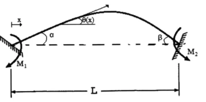
Figure 10: Angular misalignment diagram. Note that the difference in the angles of deflection at the ends results in an asymmetric peak deflection along the length of the shaft. This diagram is an exaggeration of the actual misalignment in the device: a and fl will be shown to have reasonably small values.

From the diagram, the sum of moments in static equilibrium, like in equation 3, can be taken to show that

M1 = M2 = Ma, (9)

Ma, here, being a general moment variable for this derivation. Knowing that

aM(x) = V(X), (10)

ax

it is apparent that there are no shear forces along the length of the beam given M(x) = M. Then, using

relations given in the previous derivation the angle of deflection 0(x) can be found, where

0(x) =du(x) (11)

ax

Therefore,

0(x) = Ma (12)

EI

again C1 being a constant of integration. If normal sign conventions are kept, it is apparent that 0(0) = a

and 0(L) =

#

-(a + f)EI (13) Ma = _LL

As in the linear misalignment problem, one can take equation 12 and determine a complete expression for

Given that Me is a maximum at x = 0 and Ma is constant throughout, we can consider the sum of

these to represent the maximum moment from alignment error. Then, knowing that a bending stress aM at a cross-sectional point along a shaft is given as

My (14)

I

where y is the distance from the neutral axis of a shaft (the middle), the maximum alignment error stress

can be given:

Urmax rE[(Ia + fl)L + 61e] (15)

|og |=

L2-r, here is the sample radius, as stress is at a maximum when y = r. A crucial consideration in this is that

the signs for a, fl, and 8e are not assumed to be known. It is possible that these values actually oppose

each other; in this case the stress would be diminished. Yet one must actually measure each component of

the machine to determine what signs to give each error value.

6.4 Intrinsic Sample Error

For any delicate experiment, it is necessary to consider the intrinsic error in the sample itself. As

the samples undergoing testing are commercially available Barilla no. 3 spaghetti strands, there is

manufacturing error which should initially be assumed to be at the level of process and system error until

proven otherwise. It may be the case that for research using other materials samples may be prepared to a

higher standard, commercial materials usually are not made with research purposes in mind.

With this said, it is rather difficult to form a reliable model of intrinsic error in each sample

without carefully measuring each with respect to some ideal straightness, most-likely by optical methods.

Knowing that each strand is kept within a standard of quality, an estimate of maximum error was

determined by rolling a set of strands of spaghetti with a similar initial velocity to see which would slow

down the fastest. It was hypothesized that the strands which were least straight would slow down the

fastest, checking by eye to see which looked the least straight confirmed this initial idea. This small

"winner" was found out of a group of about forty candidate strands, one end was pinned down and

various peak deviations from the surface were measured.

Figure 11: Intrinsic straightness error diagram. If at the edge of a desk one can pin down one side with a finger and find the site of largest deformation by eye and measure it carefully using a caliper. This does not. however, capture any statistical notion of straightness given a sample spaghetti strand: one would need to take multiple measurements down the length of a spaghetti to gain some first order notion of a "mean straightness". However, even more insight can be gained by considering the various directions the pasta deforms in. since much of the straightness error exists out of plane.

The most error-laden strand had a maximum deflection of about 6mm. Thus this can serve as a reasonable

bound on intrinsic error; subsequent calculations will show that this intrinsic error is rather large

compared to systemic error.

6.5 Sample Constraint Error

Another error to consider is the mounting error from clearance of the set screw sleeve for the

spaghetti. Given that each set screw was drilled using a standard #54 drill with an outer diameter of

.0550", or 1.397mm. Given a nominal spaghetti diameter of 1.393mm, assume that the clearance of the

sleeve is approximately 0.004mm. The length of the sleeve is 9.53mm, and so the maximum rotation error

is approximately 1.44 arcmin. Since there is also adhesive present in the set screw, the actual

misalignment should be less.

6.6 Friction Pivot Error

There are two last errors which whose effect on system performance must be analyzed: friction

due to the pivots and holding torque of the set screw sleeves. It is easily observed that as both pivots are

brought closer together during an experimental run, the smoothness of the rotation of the pivots begins to

degrade. Because each sample exerts a moment on the pivot to minimize any pivot angle at the ends,

the pivot increases like sin(O) 0 0 2 (classically the spaghetti breaks when the curvature _{K ~-; for}

more details, see A&N). This happens because when the force applied to the pivots goes below the frictional force of the pivot, a "stiction" (citation) phenomena emerges; the carriage can be moved a certain amount before the pivot appears to suddenly pop into place.

Fg

Ff

litetett fit fl i fe tl t

Figure 12': _{Shaft friction diagram. The model presented here is an idealized version of the actual case in question: the pivot}

prevents motion in the x and y direction and there is only one point of contact between the surface and shaft when in actuality there is area contact on the shaft.

To model this, consider the friction on a shaft resting at a point with motion limited to rotation (so no rolling can occur). Assume that an applied moment is at equilibrium with the frictional force. Then a force balance gives

Fy = 0 = N

-. (16)

F, = 0 = - IN rshaft

The gravitational force F is halved because there are two pivot points, Mf is the reaction moment due to one side of the spaghetti, r, is the radius of the shaft, N is the normal force, and M is the coefficient of friction between the shaft and pivot post. Remember that Mf is a reaction force resulting in the fact that the carriage moves a certain distance without the pivot rotating [Figure 5]. And because this error never truly disappears, there is a disparity between the ideal and actual angle, much like the linear alignment

error considered earlier. Because of the similarity between these two cases, it is convenient to use the

moment result from equation 13.

However, this angular error y has a slight caveat. In the first misalignment case, the deflection

was modeled as exactly perpendicular to the axis of the rod. Here the angle is a function of the given

angular position of the pivot. For some incremental carriage travel Ax, where Ax is defined as the

distance the carriage can travel without causing a pivot rotation, a relation

y = AxK[6(x)] (17) can be established. 6(x) here is the current angular position as a function of the carriage position on the

linear stage. K(6) represents a periodic function which relates the angular error to the incremental

carriage travel. In order to develop the motion profile of this system one would have to go and carefully

measure the pivot's angle while slowly moving the carriage. For the purpose of this experiment,

informative estimates are a more judicious use of time. Putting equations 17 and 16 together, the

minimum distance the carriage can travel given a pivot angle without overcoming the static friction is

2

LrshaftYFg (18)

Axmin _K(6)EI

Equation 18 can also be understood as a sort of system "frictional resolution", where Axmin along any

point of the carriage travel range tells of the disparity between the ideal and actual pivot angle. In the

interest of stress due to friction, equation 14 results in

SFrs aftrsample (19)

f-This stress is evaluated at the surface of the sample cross section, at rsample- Entering values for each

parameter will give an order of magnitude comparison between this and other unwanted stress

contributions.

6.7 Set Screw Sleeve Holding Torque

Lastly, holding torque of the set screw sleeves does not necessarily contribute to unwanted

Appendix, balancing grip tightness with added stress when designing a satisfactory sample holder was of considerable difficulty. Fortunately the final adhesive solution provides a strong holding force with virtually no added stress. Yet like the other gripper designs, the set screw sleeve is still liable to slippage in the rotation stage. In fact, early in system testing spaghetti samples exhibited a surprisingly high

reaction torque after being twisted more than 600. As an aside: if one were to estimate this torque, the

equation

T G_ (20)

L

provides the torque T for a given angle of deflection V. Although G, the shear modulus of the spaghetti

samples, was never experimentally determined, one can get a rough estimate assuming a Poisson's Ratio

9 of 0.3 (see Matz) and using the relation

G E (21)

2(1 + t9)'

For vp = 100', one finds a torsion of around 0.11 Nm. For comparison, the average maximum torque

generated by human hands is 2-3Nm (Arezes et al. p. 40).

Given an axial load F1, the torque Tf required to overcome the frictional force is given by

Tf=F -+= P DO + D+

9

F( 27r +2 c. s (y) 2 )'

where P is the screw pitch, Db is the nominal screw diameter, Dn is the nominal nut diameter, p, is the

coefficient of static friction, and y is the screw thread angle4_{. In reality there are two coefficients of}

friction since in the actual device the "bolt" is steel, the set screw sleeve is brass, and the preload set

screw is also steel. From equation 22 one can equate the torque to overcome the screw friction and the

torque from twisting the spaghetti sample. Then preload F, from the steel set screw can be expressed as

F JTG(O(P DbJU Dup '

Fp = - + DO + . (23)

L (27r 2 cos(y) 2

With these sets of equations a reasonable estimate of unwanted stress applied to different samples under

test. The next section describes actual measurement of the system and how they contribute to relevant

error parameters.

7 Device Measurements and Error Propagation

7.1 Description of Measurement Method

Figure 13: Diagram of measurement coordinate system locations on device. Figure is a representation of the four pivot posts. each having a coordinate system located at its respective "outer" corner. These coordinate systems were established so that measurements could be reliably made by hand. Also note that the first coordinate system serves as a reference to the others.

In this section the geometric reality of the final constructed device will be characterized and a list

of calculated parameters as well as the final error contribution will be given.

The system was measured by a 0.0 1mm resolution caliper using four reference coordinate systems, each

coordinate system at the outer-most corner of the device's four pivot posts. One coordinate system served

as a "ground" so that each pivot axis could be defined.

7.2 Pivot Axis Position and Angular Error

To determine the relative position of the two axes, the position of the centers at both shafts were

measured; for a given shaft., positon error can be defined as

(5

=

where (ij) is a pair of coordinate systems which correspond to one pivot axis, and o is the ground coordinate system. Since the first coordinate system is also the ground coordinate system, the "oi" and "oj" scripted terms drop out. There is no y-component of this position error since there is only point of interest (POI) per axis located in the middle, where the sample is purported to be held. The only y-component error is the final misalignment error between both POIs. Given the position error of each side of the axes, find the angular errors EL) at each PO:

Lais ₍₂₅₎

S =Laxis

With each axis' position and rotation errors, and also given the relative positions of each POI to the reference coordinate system, total x, y, z position errors can be established.

7.3 POI Position and Angular Error

Obtaining the final angular errors of each POI requires rotation transformation matrices since Ex and Ej _{cannot be merely added together. Consider angles 6 and y for rotations about the x and z axis,}

respectively. Then we have

1 0 0

R = 0 cos(y) -sin(y)

[

0 sin(y) cos(y)

the x-axis rotation matrix, and

rcos(6)

0

Rz= sin(6) cos(6) 0], (27)

0 0 1

the z-axis rotation matrix. Then the total rotation matrix Rtot can be obtained by multiplying the two matrices together, resulting in

cos(6) - sin(6) cos(y) sin(9) sin(y)

Rtot= sin(6) cos(6) cos(y) - sin(y) cos(6) (28)

0 sin(y) cos(y)

Tr(R) = 1 + 2cos(o)

Then,

_=

C-1 cos(y) + cos() + cos(o) cos(y) - 1 2

With co the unwanted stress due to angular alignment error can be determined.

Below, a table of values is presented to give numbers to the various relations derived above.

(30)

Parameter (add in symbols) Value Units

(y, 6z) (0.185, -0.275) mm

(a,fl) (4.7,0.28) mrad

Linear alignment error moment 0.8 N*mm

Angular alignment error moment 0.42 N*mm

Max frictional moment 3 N*mm

Linear misalignment stress .37 MPa

Angular misalignment stress .196 MPa

Pivot Friction stress 1.39 MPa

Screw preload force 2.07 N

Total First-Order Sample Error Stress 1.96 MPa

Table 2: Calculated parameters from stress characterization. Total stress given is about one-seventh of the allowable stress on the sample.

8 Future Considerations

8.1 Device Improvements

While the experiment this device initially serves requires a high-speed camera to monitor the amount of fracture events that happen after the first fracture, other applications of the device may very well be served by the incorporation of sensors into the device. For example, one might be interested in investigating how different initial twisting angles affect the reaction force at the ends of the spaghetti (or

other thin material) as two ends are brought closer together. On the other hand, one might want to investigate whether the torque from torsion changes as the two ends are brought together. Since the spaghetti undergo large deformations it is not necessarily evident what the profile of reaction torques and forces would be, assuming that both are simultaneously present in the system.

With current design of the device, the interface between the pivots and pivot posts would have to include space for a sensor compatible with the rotating feature of this component. For a torsional sensor, a new rotation mount would need to be chosen, unless a solution with a reasonable weight could be

implemented.

Figure 14: Image of final device displaying underside of pivots. One can see the metal rods protruding from the back of the rotary stage. When the spaghetti collets were being tested the backside would be secured using pliers and the dial on the rotary mount would be twisted until a sample was sufficiently tightened. Additionally one may be able to see writing on the pivot: it was found that marking the components of the machine aided in making measurements and keeping track of relative position components.

One can always choose higher precision motion stages to have a finer resolution experiment. This may be necessary for doing similar testing to thinner, weaker, or more brittle materials. These

improvements would go hand-in-hand with the desire to incorporate other sensors into the experimental system.