HAL Id: hal-01839334
https://hal-univ-rennes1.archives-ouvertes.fr/hal-01839334
Submitted on 10 Sep 2018
HAL is a multi-disciplinary open access
archive for the deposit and dissemination of sci-entific research documents, whether they are pub-lished or not. The documents may come from teaching and research institutions in France or
L’archive ouverte pluridisciplinaire HAL, est destinée au dépôt et à la diffusion de documents scientifiques de niveau recherche, publiés ou non, émanant des établissements d’enseignement et de recherche français ou étrangers, des laboratoires
Yang, Lotfi Senhadji, Huazhong Shu
To cite this version:
Jiasong Wu, Shijie Qiu, Youyong Kong, Longyu Jiang, Yang Chen, et al.. PCANet: An energy perspective. Neurocomputing, Elsevier, 2018, 313, pp.271-287. �10.1016/j.neucom.2018.06.025�. �hal-01839334�
ACCEPTED MANUSCRIPT
PCANet: An energy perspective
Jiasong Wu1, 2, 4, Shijie Qiu1, 4, Youyong Kong1, 4, Longyu Jiang1, 4,
Yang Chen1, 4, Wankou Yang5, Lotfi Senhadji3, 4, Huazhong Shu1, 2, 4
1
LIST, Key Laboratory of Computer Network and Information Integration, Southeast University, Ministry of
Education, Nanjing 210096, China
2
International Joint Research Laboratory of Information Display and Visualization, Southeast University, Ministry
of Education, Nanjing 210096, China
3
Univ Rennes, INSERM, LTSI - UMR 1099, F-35000 Rennes, France
4
Centre de Recherche en Information Biomédicale Sino-français (CRIBs), SEU, Univ Rennes, INSERM, Nanjing
210096, China
5
School of Automation, Southeast University, Nanjing 210096, China
Abstract
The principal component analysis network (PCANet), which is one of the recently proposed deep learning
architectures, achieves the state-of-the-art classification accuracy in various databases. However, the visualization or
explanation of the PCANet is lacked. In this paper, we try to explain why PCANet works well from energy perspective
point of view based on a set of experiments. The paper shows that the error rate of PCANet is qualitatively correlated
with the inverse of the logarithm of BlockEnergy, which is the energy after the block sliding process of PCANet, and
also this relation is quantified by using curve fitting method. The proposed energy explanation approach can also be
used as a testing method for checking if every step of the constructed networks is necessary.
Keywords
ACCEPTED MANUSCRIPT
1. Introduction
Deep learning [1-10], especially convolutional neural networks (CNNs) [11, 12], is a hot research topic that
achieves the state-of-the-art results in many image classification tasks, including ImageNet large scale visual
recognition [13-17], Labeled Faces in the Wild (LFW) face recognition [18-20], handwritten digit recognition [11, 21],
and other applications [22-31], etc. The great success of deep learning systems is impressive, but a fundamental
question still remains: Why do they work [32]? In the recent years, several attempts have been made for explaining the
deep learning systems. These attempts can be roughly categorized into two classes: theoretical explanation and
experimental explanation.
Theoretical explanation method tries to elucidate deep learning systems by using various theories, which can be
classified into seven subclasses: 1) Renormalization Theory. Mehta and Schwab [33] constructed an exact mapping
from the variational renormalization group (RG) scheme [34] to deep neural networks (DNNs) based on Restricted
Boltzmann Machines (RBMs) [1, 2], and thus explained DNNs as a RG-like procedure to extract relevant features from
structured data. 2) Probabilistic Theory. Patel et al. [32] developed a new probabilistic framework for deep learning
based on a Bayesian generative probabilistic model. By relaxing the generative model to a discriminative one, their
models recover two of the current leading deep learning systems: deep CNNs and random decision forests (RDFs). 3)
Information Theory. Tishby and Zaslavsky [35] analyzed DNNs via the theoretical framework of the information
bottleneck principle. Steeg and Galstyan [36] further introduced a framework for unsupervised learning of deep
representations based on a hierarchical decomposition of information. 4) Developmental robotic perspective. Sigaud
and Droniou [37] scrutinized deep learning techniques under the light of their capability to construct a hierarchy of
multimodal representations from the raw sensors of robots. 5) Geometric viewpoint. Lei et al. [38] showed the intrinsic
relations between optimal transportation and convex geometry and gave a geometric interpretation to generative
models. Dong et al. [39] draw a geometric picture of the deep learning system by finding its analogies with two existing geometric structures, the geometry of quantum computations and the geometry of the diffeomorphic template
matching. 6) Group Theory. Paul and Venkatasubramanian [40] explained deep learning system from the
group-theoretic perspective point of view and showed why higher layers of deep learning framework tend to learn more
abstract features. Shaham et al. [41] discussed the approximation of wavelet functions using deep neural nets. Anselmi
ACCEPTED MANUSCRIPT
recent theory of feedforward processing in sensory cortex. 7) Energy perspective. The mathematical analysis of CNNs
was performed by Mallat in [44], where wavelet scattering network (ScatNet) was proposed. The convolutional layer,
nonlinear layer, pooling layer were constructed by prefixed complex wavelets, modulus operator, and average operator,
respectively. Owning to its characteristic of using prefixed filters which are not learned from data, ScatNet was
explained in [44] from energy perspective both in theory and experiment aspect, that is, ScatNet maintains the energy
of image in each layer although using modulus operator. ScatNet achieves the state-of-the-art results in various
image classification tasks [45] and was then extended to semi-discrete frame networks [46] as well as complex valued
convolutional nets [47].
Experimental explanation methods tend to understand deep learning systems by inverting them to visualize the
“filters” learned by the model [48]. For example, Larochelle et al. [49] presented a series of experiments on Deep Belief Networks (DBN) [1] and stacked autoencoder networks [3] by using artificial data and indicate that these models
show promise in solving harder learning problems that exhibit many factors of variation. Goodfellow et al. [50]
examined the invariances of stacked autoencoder networks [3] and also convolutional deep belief networks (CDBNs)
[4] by using natural images and natural video sequences. Erhan et al. [48] studied three filter visualization methods
(Maximizing the activation, Sampling from a unit of a network, Linear combination of previous layers‟ filters) on DBN [1] and Stacked Denoising Autoencoders [5]. Szegedy et al. [51] reported two intriguing properties of deep neural
networks. Zeiler and Fergus [52] proposed DeConvNet method in which the network computations were backtracked
to identify which image patches are responsible for certain neural activations. DeConvNet uses AlexNet [11] as an
example to observe the evolution of features during training and to diagnose potential problems by using such a model.
Simonyan et al. [53] demonstrated how saliency maps can be obtained from a Convnet by projecting back from the
fully connected layers of the network. Girshick et al. [54] showed visualizations that identify patches within a dataset
that are responsible for strong activations at higher layers in the model. Mahendran and Vedaldi [55] gave a general
framework to invert CNNs and they tried to answer the following question: given an encoding of an image, to which
extent is it possible to reconstruct the image itself?
Recently, Chan et al. [56] proposed a new deep learning algorithm called principal component analysis network
(PCANet), whose convolutional layer, nonlinear processing layer, and feature pooling layer consist of principal
ACCEPTED MANUSCRIPT
visualize the filters of PCANet like in [48] and [52]. Although PCANet is constructed with most basic units, it
surprisingly achieves the state-of-the-art performance for most image classification tasks. PCANet arouses the interest
of many researchers in this field. For example, Gan et al. proposed a graph embedding network (GENet) [57] for image
classification. Wang and Tan [58] presented a C-SVDDNet for unsupervised feature learning. Feng et al. [59]
presented a discriminative locality alignment network (DLANet) for scene classification. Ng and Teoh [60] proposed
discrete cosine transform network (DCTNet) for face recognition. Gan et al. [61] presented a PCA-based convolutional
network by combining the structure of PCANet and the LeNet-5 [11, 12]. Zhao et al. [62] proposed multi-level
modified finite radon transform network (MMFRTN) for image upsampling. Lei et al. [63] developed stacked image
descriptor for face recognition. Li et al. [64] proposed SAE-PCA network for human gesture recognition in RGBD
(Red, Green, Blue, Depth) images. Zeng et al. [65] proposed a quaternion principal component analysis network
(QPCANet) for color image classification. Wu et al. [66] proposed a multilinear principal component analysis network
(MPCANet) for tensor object classification. Although PCANet has been extensively investigated, the question still
remains: Why it works well by using the most basic and simple units? To the best of our knowledge, no attempt to
explain every step of the PCANet is available in the literature.
In this paper, 1) We present a new way to visualize, explain and understand every step of PCANet from an energy
perspective on experiment aspect by using five image databases: Yale database [67], AR database [68], CMU PIE face
database [69], ORL database [70], and CIFAR-10 database [71]. The proposed energy explanation approach can
provide more information than the filter visualization method reported in [56]; 2) We shows qualitatively that the error
rate of PCANet is correlated with the inverse of the logarithm of BlockEnergy, which is the energy after the block
sliding process of PCANet, and then we try to find quantitatively their relations by using curve fitting method; 3) we
show that the proposed energy explanation approach can be used as a testing method for checking if every step of the
constructed networks is necessary; and 4) The energy explanation approach proposed in this paper can be extended to
other PCANet-based networks [57-66].
The paper is organized as follows. PCANet is reviewed in section 2. Section 3 presents an energy method to
visualize, explain and understand every step of PCANet. Discussion is given in Section 4 and Section 5 concludes the
ACCEPTED MANUSCRIPT
2.Review of Principal Component Analysis Network
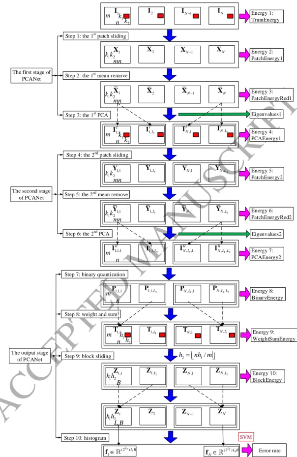
In this section, we first review the PCANet [56], whose architecture is shown in Fig. 1 and can be divided into
three stages, including 10 steps. Suppose that we have N input training images
Ii,i1, 2,...,N
, Ii m n , and that the patch size (or two-dimensional filter size) of all stages is k1×k2, where k1 and k2 are odd integers satisfying 1≤k1≤m,1≤k2≤n. We further assume that the number of filters in layer i is Li, that is, L1 for the first stage and L2 for the second
stage. In the following, we describe the structure of PCANet in detail.
Let the N input images
Ii,i1, 2,...,N
be concatenated as follows:
1 2
m Nn N I I I I . (1)2.1. The first stage of PCANet
As shown in Fig. 1, the first stage of PCANet includes the following 3 steps:
Step 1: the first patch sliding process.
The images are padded to (m k1 1) (n k2 1)
i
I before sliding operation. Out-of-range input pixels are taken to be
zero. This can ensure all weights in the filters reach the entire images. We use a patch of size k1×k2 to slide each pixel of
the ith image (m k1 1) (n k2 1)
i
I , then reshape each k1×k2 matrix into a column vector, which is then concatenated to
obtain a matrix 1 2 ,1 ,2 , , 1, 2,..., , k k mn i i i i mn i N X x x x (2)
where xi,j denotes the jth vectorized patch in Ii.
Therefore, for all the input training images
Ii,i1, 2,...,N
, we can obtain the following matrix
1 2 1 2 , k k Nmn N X X X X (3)Step 2: the first mean remove process.
In this step, we subtract patch mean from each patch and obtain
1 2 ,1 ,2 , , 1, 2,..., , k k mn i i i i mn i N X x x x (4) where , , , 1 1 , mn i j i j i j j mn
x x x is a mean-removed vector.ACCEPTED MANUSCRIPT
For each input training image m n i
I , we can get a substituted matrix k k1 2 mn
i
X . Thus, for all the input
training images
Ii,i1, 2,...,N
, we can obtain the following matrix 1 2 1 2 . k k Nmn N X X X X (5)Step 3: the first PCA process.
In this step, we get the eigenvalues and eigenvectors of X in (5) by using PCA algorithm, which in fact minimizes the reconstruction error in Frobenius norm as follows:
1 1 2 1 2 min , s.t. , k k L T T L F U X UU X U U D (6) where 1 L
D is an identity matrix of size L1×L1, and the superscript T denotes transposition. Eq. (6) can be solved by
eigenvalue decomposition method shown in Appendix. The PCA filter of the first stage of PCANet is then obtained
from (A.5) by
1 2 1,2 1 mat k k , 1, 2, , , I l k k l l L W u (7)wherematk k1,2
ul is a function that maps k k1 2l
u to a matrix I k1 k2
l
W . Note that the superscript of capital Roman
number I denotes the first stage,
The output of the first stage of PCANet is given by
, , 1, 2,..., ; 1 1, 2, , , I I m n i l i l l L i N I I W (8) where ∗ denotes two-dimensional (2-D) convolution, and the boundary of Ii is zero-padded before convolving with WlI
in order to make I, i l
I having the same size as Ii.
For each input image m n
i
I , we obtain L1 output images
,, 1, 2,..., 1
, ,I I m n
i l l L i l
I I after the first stage of
PCANet. We denote II as 1 1 1 1,1 1, ,1 , m NL n I I I I I L N N L I I I I I . (9)
2.2. The second stage of PCANet
As shown in Fig. 1, the second stage of PCANet also includes 3 steps:
ACCEPTED MANUSCRIPT
Similar to Step 1, we use a patch of size k1×k2 to slide each pixel of the ith image , 1 2, 1, 2,..., 1
k k I i l l L I , and obtain a matrix 1 2 , , ,1 , ,2 , , , 1, 2,..., 1; 1, 2,..., , k k mn i l i l i l i l mn l L i N Y y y y (10)
where yi l j, , denotes the jth vectorized patch in I, i l
I .
Therefore, for the ith filter, all the input training images
I,, 1, 2,...,
i l i N
I , we can obtain the following matrix
1 2 1, 2, , , k k Nmn l l l N l Y Y Y Y (11)
We concatenate the matrices of all the L1 filters and obtain
1 2 1 1 1 2 . k k L Nmn L Y Y Y Y (12)
Step 5: the second mean remove process.
Similar to Step 2, we obtain the mean-removed version of (12) by
1 2 1 1 1 2 , 1, 2,..., ,1 k k L Nmn L l L Y Y Y Y (13) where 1 2 1, 2, , , k k Nmn l l l N l Y Y Y Y (14) 1 2 , , ,1 , ,2 , , , 1, 2,..., 1; 1, 2,..., , k k mn i l i l i l i l mn l L i N Y y y y (15) , , , , , , 1 1 1 , 1, 2,..., ; 1, 2,..., . mn i l j i l j i l j j l L i N mn
y y y (16)Step 6: the second PCA process.
Similar to Step 3, we use the PCA algorithm to minimize the following optimization problem:
2 1 2 2 2 min , s.t. , k k L T T L F V Y VV Y V V D (17) where 2 L
D is an identity matrix of size L2×L2. Eq. (17) can also be solved by the eigenvalue decomposition method
shown in Appendix in which we replace , , , 1, , , 1 I, 1, 2,..., 1
i L N i L X U u C by , , , 2, 2, 1 , II, 1, 2,..., 2 i L L N i L Y V v C ,
respectively. The PCA filter of the second stage of PCANet is then obtained from (A.5) by
1 2 1,2 2 mat k k , 1, 2, , , II k k L W v (18)ACCEPTED MANUSCRIPT
where
1,2
matk k v is a function that maps v k k1 2 to a matrix WII k1k2. Note that the italic superscript II in (18) denotes the second stage. Therefore, the output of the second stage of PCANet is given by
1 2 , , , , 1, 2,..., 1; 1, 2,..., 2; 1, 2, , , k k II I II i l i l l L L i N I I W (19)
where ∗ denotes 2-D convolution.
For each input image I, m n
i l
I , we obtain L2 output images
, ,, 1, 2,..., 2
, , ,II II m n
i l L i l
I I after the second stage
of PCANet. Thus, we obtain NL1L2 images
, , 1, 2,..., 1; 1, 2,..., 2; 1, 2, ,
, , , ,II II m n
i l l L L i N i l
I , I for all the input
training images
, 1, 2, ,
, m ni i N i
I I after the first and second stages.
We denote III as 2 1 1 2 2 1 1 2 1,1,1 1,1, 1, ,1 1, , ,1,1 ,1, , ,1 , , . II II II II II II II II II L L L L N N L N L N L L I I I I I I I I I (20)
2.3. The output stage of PCANet Step 7: binary quantization.
In this step, we binarize the outputs , , II i l
I of the second stage of PCANet and obtain
, , , , , 1, 2,..., 1; 1, 2,..., 2; 1, 2, , , II i l H i l l L L i N P I (21)where H(·) is a Heaviside step function whose value is one for positive entries and zero otherwise. We denote P as
2 1 1 2 2 1 1 2
1,1,1 1,1,L 1,L,1 1,L L, N,1,1 N,1,L N L, ,1 N L L, , .
P P P P P P P P P (22)
Step 8: weight and sum.
Around each pixel, we view the vector of L2binary bits as a decimal number. This converts the binary images
Pi l, ,
back into integer-valued images as follows:2 1 , , , 1 2 , L i l i l
T P (23) We denote T as 1 1 1 1,1 1, ,1 , m NL n L N N L T T T T T . (24)ACCEPTED MANUSCRIPT
We use a block of size h1×h2 to slide each of the L1 images Ti l,,l1,...,L1, with overlap ratio R, and then reshape each h1×h2 matrix into a columnvector, which is then concatenated to obtain a matrix
1 2 , , ,1 , ,2 , , , 1, 2,..., , h h B i l i l i l i l B i N Z z z z (25)
where zi,l,j denotes the jth vectorized patch in Ti l,,l1,...,L1. B is the number of blocks when using a block of size h1×h2 to slide each Ti l,,l1,...,L1,with overlap ratio R and given by
1 1
2 2
1 1 / stride1 1 1 / stride2
B m k h n k h ,
(26)
where stride1 and stride2 are vertical and horizontal steps, respectively,
1
stride1round 1R h , (27)
2
stride2round 1R h , (28)and round (.) means round off. As we can see from (26)-(28), the number of blocks B is increasing as the overlap ratio
R is increasing.
For L1 images, we concatenate Zi l, to obtain a matrix
1 2 1 ,1 ,2 , , 1, 2,..., , h h L B i i i i B i N Z Z Z Z (29) We denote Z as 1 2 1 1,1 1, ,1 , . h h L BN B N N B Z Z Z Z Z (30) Step 10: histogram.
We compute the histogram (with 2L2 bins) of the decimal values in each column of Z
i and concatenate all the
histograms into one vector and obtain
2 1
1 1
(2 )
,1,1 ,1, , ,1 , ,
Hist( ) Hist( ) Hist( ) Hist( ) T L L B.
i i i B i L i L B
f z z z z (31)
which is the “feature” of the input image Ii and Hist(.) denotes the histogram operation. We denote f as
2 1 (2 ) 1 L L BN N f f f . (32)The feature vector is then sent to a classifier, for example, support vector machine (SVM) [72], k-nearest
ACCEPTED MANUSCRIPT
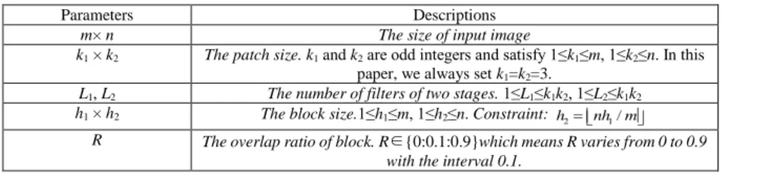
2.4. The parameters of PCANet
The dimension of PCANet feature is related to the core parameters shown in Table 1. For a given dataset, m and n
are fixed. In this paper, we always set k1=k2=3 since in this case the consumption of memory is tolerable for an ordinary
computer (for example, 64 GB RAM). Note also that we set a constraint
2 1/
h nh m, (33)
which is a common choice in practice. After the above setting, there are four free parameters left: L1, L2, h1, and R.
3. Energy Analysis and Energy Explanation of PCANet
In this section, we introduce the details of the proposed energy explanation approach method. We first present the
motivation of the proposed approach, and then we describe the experiment methods and the used databases. The
following experiments were implemented in Matlab programming language.
3.1. Motivations
CNNs are visualized and understood by using back-trace or inverted method to show the filters (or weights) that
are learned by every layer [48, 52, 55]. The filters show much information since CNNs generally have many layers and
the number of these filters are very large. Chan et al. [56] also visualize the filters of PCANet like in [48], [52], and
[55]. However, PCANet does not have such large number of filters like CNNs, therefore, visualizing the filters only
provides limited information about two filter layers (Steps 3 and 6) of PCANet. Furthermore, how to effectively
visualize other implemental steps (Steps 1, 2, 4, 5, and 7-9) of PCANet is still an open problem since these simple
operations have a prominent impact on the performance of PCANet. For example, as depicted in [56], the performance
of PCANet is degraded if we delete the simple mean-remove process.
On the one hand, PCA, also known as Karhunen-Loeve transform (KLT), is very popular in data compression
domain since it has very good energy concentration capability, that is, few coefficients of KLT capture vast majority of
energy of the original signal. On the other hand, Mallat and Bruna [44, 45] also prove and explain ScatNet from energy
perspective. However, there are two main differences between PCANet and ScatNet [44, 45]: (1) the convolutional
layer of PCANet is constructed by data-dependent PCA filter while the convolutional layer of ScatNet is constructed by
data-free complex wavelet filter; (2) the nonlinearity of PCANet is binarization while the nonlinearity of ScatNet is
ACCEPTED MANUSCRIPT
perspective?
3.2. Experiment databases
In the following, we use five databases, whose Matlab formats are provided in [71] and [74], to analyze the energy
change as well as the error rate change of PCANet: 1) Yale database [67]. It contains 165 grayscale images (15
individuals, 11 images per individual), which are randomly divided into 30 training images and 135 testing images; 2)
AR database [68]. We use a non-occluded subset of AR database containing 700 images (50 male subjects, 14 images
per subject), which are randomly divided into 200 training images and 500 testing images; 3) The CMU PIE face
database [69]. We use pose C27 (a frontal pose) subset of CMU PIE face database which has 3400 images (68 persons,
50 images per person), which are randomly divided into 1000 training images and 2400 testing images; 4) ORL
database [70]. It contains 400 grayscale images (40 individuals, 10 images per individual), which are randomly
divided into 80 training images and 320 testing images. 5) CIFAR-10 database [71]. The original database contains
60000 color images (10 classes), including 50000 training images and 10000 test images. In our experiment, we
randomly choose 3000 images for training and 1000 images for testing. Note that the size of all the images is 32×32
pixels. For the cross validation, we use the simplest hold-out validation due to the following two reasons: 1) some cases
of the experiments are time and memory consuming; 2) the objective of the paper is not to achieve the lowest error rate
but to establish the one-to-one correspondence of error rate e and the inverse of the logarithm of BlockEnergy g, and
then find the parameters to achieve the relatively low error rate by the guidance of energy. Therefore, we need e and g
are directly correspondent.
3.3. Experiment methods
In this section, we exploit the above-mentioned databases to analyze the PCANet by using energy method. We
first introduce the definition of the energy of a two-dimensional image I (i, j) of size m×n:
2 1 1 ( ) ( , ) m n i j E i j
I I . (34)Fig. 1 shows that we record 10 energies for PCANet. It is convenient for us to divide these energies into two parts:
Energies 1-9 belong to the first part and Energy 10 belongs to the second part. The reason for this partitioning is that
Energies 1-9 are not related to the block size h1 × h2 and the overlap ratio R. The values that we recorded in the whole
ACCEPTED MANUSCRIPT
energy of the feature f in (32) into consideration, since the block-wise histogram is only the statistic (or occurrence
frequency) of energy value and we consider that this process does not change the energy.
3.3.1 The analysis of the second part
In this subsection, we first introduce two metrics of the experiments. The first metric is the inverse of the logarithm
of BlockEnergy E(Z), shown in Table 2, that is
10
1 / log ( )
g E Z . (35) The second metric is the error rate
The number of false classified testing images The total number of testing images
e . (36)
In the second part, there are 4 free parameters: h1 (the number of rows of block), R (the overlap ratio), L1 (the
number of filters of the 1st stage), L2 (the number of filters of the 2nd stage). Therefore, the aim of this subsection is to
explore qualitatively the metric g and also the metric e with regards to the parameters h1, R, L1, and L2.
1) How the g and the e qualitatively vary according to h1, R, L1, and L2?
In this experiment, we use Yale database for analyzing the g and also the e in relation with h1, R, L1, L2, where
h1{1:1:32}, R{0:0.1:0.9}, and L1, L2{1:1:9}. Note that {a:b:c} means the set contains the values that vary from a
to c with increment b. Each combination of h1, L1, L2, and R has a e value or g value. Therefore, if we denote M as the
total number of e or g, then, M=32×10×9×9=25920.
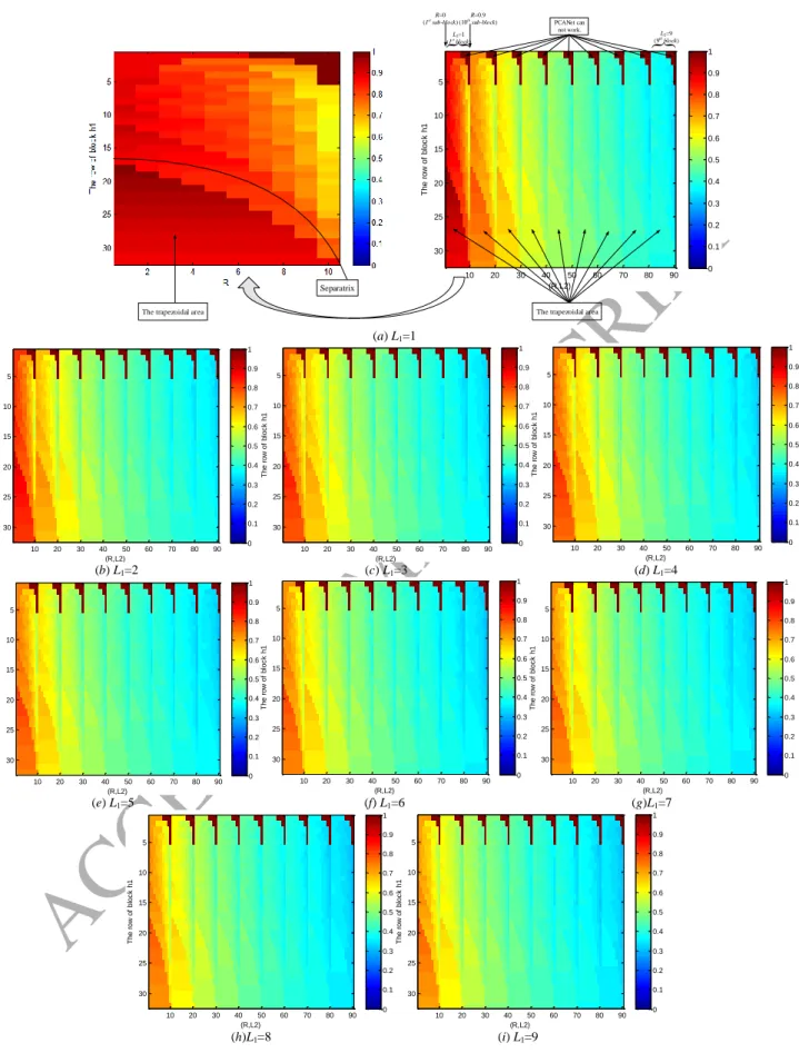
The results of the variations of g according to h1, R, L1, L2 are shown in Fig. 2, whose vertical axis is h1{1:1:32}
and horizontal axis is related to R and L2. Specifically, the horizontal axis can be divided into 9 blocks corresponding to
L2{1:1:9}, each block can further be divided into 10 sub-blocks corresponding to R{0:0.1:0.9}, where each sub-block has the size of 32×1. Therefore, the range of horizontal axis value is from 1 to 90 (=10×9). Fig. 2(a) is in fact
the concatenated version of 90 images. In Fig. 2, g is expressed by colors. The brown and the blue denote the values 1
and 0, respectively. The pure brown area appears in the figure in fact denotes that the algorithm cannot work in these
cases, specifically, the function of "HashingHist" in the PCANet software can not deal with these cases, we manually
set g=1. It does not matter, the pure brown areas are just used in Fig. 2 as separators of the results of various L2. The
ACCEPTED MANUSCRIPT
a) The impact of L1 on g and e. Both Fig. 2 and Fig. 3 contain 9 similar figures corresponding to L1{1:1:9}. If we
fix L2 and increase L1, then, both g and e are gradually decreased. When L1≥4, the figures are flattened. The first three
figures have notable changes, this phenomenon implies that the first few number of filters captures most of the energies
of the original image, leading to the severe changes of g and e.
b) The impact of L2 on g and e. As the value of L2 increases, the first five figures corresponding to L2{1:1:5}
change a lot, but when L2≥6, the left four figures only make little changes. Therefore, we can think that when L2 = 6,
both g and e are stable.
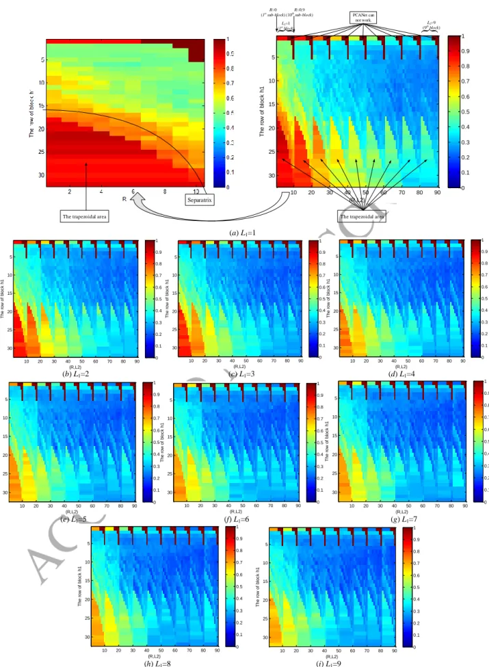
c) The impact of R on g and e. There are some differences of the changes of g and e according to R. From Fig. 2,
we can see that g is gradually decreased as the value of R increases. However, from Fig. 3, the probability of lower error
rate e is increased as the value of R increases from 0 to 0.9 with interval of 0.1. Nonetheless, the appropriate values of
R in fact belong to {0:0.1:0.6}, due to the following two reasons: Firstly, from the experimental aspect, when R≥0.7, it
may encounter the cases where PCANet can not work; When R≥0.7, the result is also good if it does not encounter the
cases where PCANet can not work, but both the computational and the memory complexities are very high from
experiment aspect since they lead to too much overlap. Let us take Yale database for example, setting k1=k2=3,
L1=L2=8, h1=h2=8, Table 3 shows the accuracy, time consumption, and dimension of features when R varies from 0 to
0.9. Secondly, from the theory or explanation aspect, the overlap ratio R has a similar role with the eigenvector in PCA
filtering as shown in Appendix. In the case of realizing dimension reduction by PCA, we want to use as few as possible
eigenvectors while keeping enough useful features of original image. Similarly, we want to use as small as possible
overlap ratio R.
d) The impact of h1 on g and e.
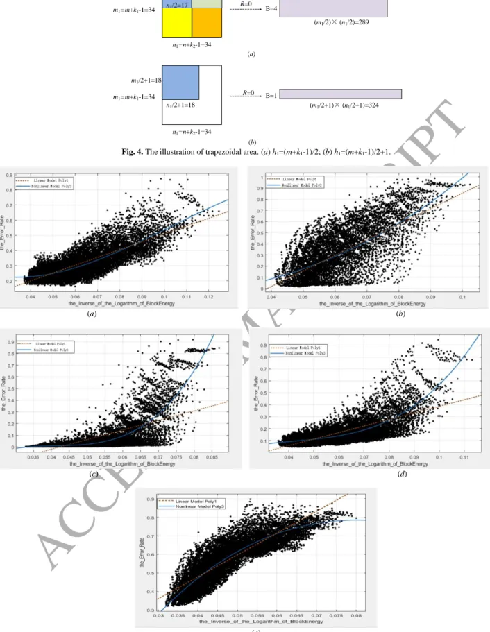
As we can see, when h1 is higher than a critical value (m+k1-1)/2+10R, each block has an obvious trapezoidal
area, where the values of g and e are evidently higher than other parts of the block. The reason is that the block sliding
process (Step 9) leads to “great reduction in energy” when h1>(m+k1-1)/2+10R. Why this phenomenon appears? Let us
take R=0 as an example, in this case, the critical value (m+k1-1)/2+10R=(32+3-1)/2+10×0=17. Figs. 4 (a) and (b) show
the case of block sliding process of h1=17 and h1=18, respectively. From Fig. 4 (a), the image of 34×34 becomes an
ACCEPTED MANUSCRIPT
is used through 3 times of block sliding process. However, as we can see from Fig. 4 (b), the image of 34×34 becomes
an image of 1×324 by block sliding process with block of 18×18. Note that both the right side and the bottom side of
the 18×18 block are not enough for a new block sliding process. In this case, we only use the information (or energy) of
18×18 block on the upper left corner, other information (or energy) of the image is not used. That is to say, the
trapezoidal area is caused by “not making full use of energy”. Therefore, the appropriate choice of the number of rows
of block is h1≤(m+k1-1)/2+10R since it can avoid the trapezoidal area.
In total, we can see the following things:
i) The changes of g and e have similar overall consistent trends, for example, the values of g and e are gradually
decreased as the value of L1 and L2 increase.
ii) The changes of g are relatively smooth, while the changes of e seem more varied than that of g. Furthermore, e
is not simply directly proportional to g.
2) How the e varies quantitatively according to g ?
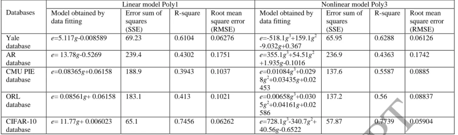
In the following, we use the Curve Fitting Tool of Matlab to further investigate the correlation between e and g.
We fit the function e = f(g), by using the linear model Poly1 and the nonlinear model Poly3 in Matlab with 95%
confidence bounds, that is, we used e = p1g+p2, and e =p3g 3
+p4g 2
+p5g+p6, where pi, i =1,2,…,6, are the coefficients to
fit, to find the relationship of e and g, respectively. The curve fitting results of five datasets are shown in Fig. 5 and the
quantitative results are shown in Table 4. The criterions include:
a) The sum of error squares (SSE), sum of regression squares (SSR), and total sum of squares (SST) are defined
respectively as 2 1 ( i ( ))i i M SSE e f g
, (37) 2 1 ( ( ) ) i M i SSR f g e
, (38) 2 1 ( i ) i M SST SSE SSR e e
, (39)ACCEPTED MANUSCRIPT
where 1 1 i i M M e e
, and i is the index of the number of e or g, and M is the total number of e or g. In our experiment,M=32×10×9×9=25920.
b) Coefficient of determination or R-square is defined as
2
1 SSE r
SST
, (40) which is a number that indicates how well data fit a statistical model, for example, a curve.
c) Root mean squared error (RMSE) is defined as
2 1 ( ( )) N i i i e f g RMSE N
. (41) As we can see from Table 4, the R-square of the data of Yale database by using linear model Poly1 is 0.6104,which means 61.04% of the variance in the response variable can be explained by the explanatory variables. Therefore,
e and g are fairly linearly correlated. As we mentioned above that the changes of g and e have similar overall consistent
trends but the changes of e seem more varied than that of g. Can we use a little more complicated model for describing
the correlation between e and g? We then use a nonlinear polynomial function of degree 3 (Poly3) to model the
relationships of e and g. The R-square of the data of Yale database by using model Poly3 is 0.6288, which means
62.88% of the variance in the response variable can be explained by the explanatory variables. The remaining 37.12%
can be attributed to unknown, lurking variables or inherent variability. Therefore, e and g are fairly non-linearly
correlated. We also give the curve fitting results for the data of five databases (Yale, AR, CMU PIE, ORL, CIFAR-10)
in Table 4. Similar conclusion can be obtained for the other databases. In fact, if we cancel the constraint in (33) and do
the similar experiment on Yale database, the R-square of the data of Yale database by using Poly3 increases further to
0.7637, which is even larger than 0.6288 that has the constraint in (33).
3) How to explain the block sliding process?
We can in fact explain this process as an “overlap filtering”, which is a term that we proposed in this paper to explain and better understand the sliding process, including the patch sliding process and the block sliding process. The
idea of “overlap filtering” is in fact from the PCA filter. The comparison and the connection of “overlap filtering” and
ACCEPTED MANUSCRIPT
3.3.2 The analysis of the first part
In this subsection, we will analyze the changes of Energies 1-9 of the first part of PCANet shown in Fig. 1. Since
the first part is not related to h1, h2, and R, so in the experiment of this section, we simply set the parameters h1 = h2 = 8,
and R= 0.5, due to the following three reasons: (1) they are near one of the recommended parameters h1 =8, h2 = 6, and
R= 0.5 in PCANet [56]; (2) they have the moderate computational complexity and memory complexity; (3) they satisfy
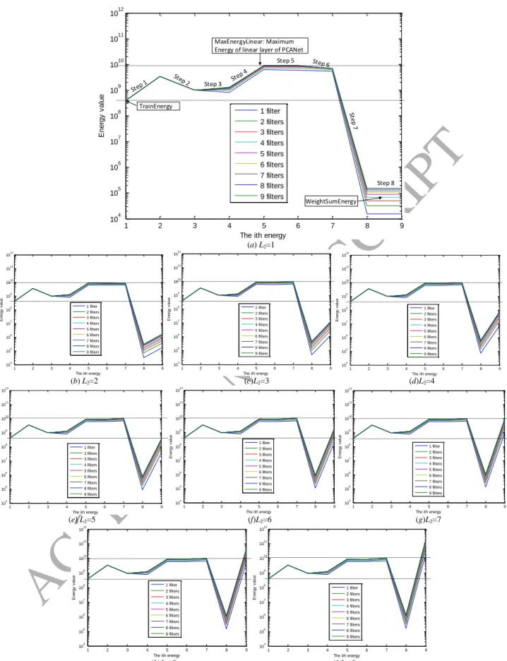
the constraint h2 nh1/min (33) in the analysis of the second part. Let us take Yale dataset as an example, Fig. 6
shows the energy values of every stage of the first part of PCANet versus the ith energy. The results of 9 filters,
corresponding to L1{1:1:9}, are shown in different colors. For example, the lowest line is the result that we choose only the largest eigenvector corresponding to L1=1. The second lowest line is the result that we choose the 2 largest
eigenvectors corresponding to L1=2, and so on. Note that the vertical axis is shown in logarithmic coordinate. From Fig.
6, for all the 9 filters, we can easily see that the energy changes are as follows
Step 1 Step 2 or Step 7 3 Step 4 Step 5 or Step 6 Step t 8 S ep 1 1 1 2 2 2 0 PatchEnergy PatchEnergyRed PCAEnergy PatchEnergy PatchEnergyRed PCAEnergy Binar TrainEnergy yEnergy , WeightSumEnergy (42)
where the arrow means that the energy values change from the left-hand side to the right-hand side. “+”, “–”, “0” above
the arrow denote the energy increase, decrease, and equal process, respectively. Steps 1-8 below the arrow correspond
to the eight steps of Fig. 1.
From (42), we can see that:
1) For Steps 1 and 4, both of them are energy increasing processes, which can be easily understood since these
two steps perform the overlapping patch sliding process. However, how can we explain the patch sliding process? In
fact, the patch sliding process is a special case of block sliding process with the overlap ratio R=0.9 shown in the
second part.
2) For the Steps 2 and 5, both of them are mean removing processes. Step 2 is energy decreasing process, which is
ACCEPTED MANUSCRIPT
the energy. Therefore, we think this step may not be needed in the construction of PCANet. We then perform
some experiments on four databases to verify our inference. We compute the differences of error rates of PCANet with
mean remove Step 5 and that of without Step 5 for all the parameter setting of h1{1:1:32}, R{0:0.1:0.9}, and L1,
L2{1:1:9}. The mean of differences of error rates for Yale database, AR database, CMU PIE database, and ORL database are 1.1762×10⁻⁶, 1.5878×10⁻⁷, -1.4886×10⁻⁷, -4.9619×10⁻⁷, respectively, all of which are very small.
Therefore, when taking the computational complexity into consideration, we recommend to not use the mean remove process of Step 5.
3) For the Steps 3 and 6, both of them are PCA processes. Both Step 3 and Step 6 are energy increasing processes
except the case of 1 filter, but the energy change is very small. Table 6 shows the energy of each of the 9 filters (the 1st
PCA), h1=h2=8, R=0.5, L2=1, and L1 varies from 1 to 9, and the energy of every filter (the 2nd PCA), h1=h2=8, R=0.5,
L1=8, and L2 varies from 1 to 9. Table 7 shows the error rate corresponding to L1, L2∈{1:1:9} when h1=h2=8, R=0.5.
From the two Tables, we can see that the cumulative percentage of eigenvalue can be a guideline for the choice of L1
and L2, for example, the error rate of Yale database is low when the cumulative percentage of eigenvalue is larger than
99.7%, which corresponds to L1=8 and L2=8. Note that L1=L2=8 is just one of the parameter settings recommended by
Chan‟s paper [56].
4) For the Steps 7 and 8, which cause the sharpest energy changes of PCANet. It is also reasonable since the
binarization operation is a very powerful quantization process (nonlinear processing), which loses much energy.
Meanwhile, the weighted and summed step is a very powerful energy increasing step. It is interesting to see from Fig. 6
that the energy in Step 8 gradually increases when L2 varies from 1 to 9. Let's focus on the two horizontal dashed lines:
the first one denotes the MaxEnergyLinear (maximum energy of linear layer of PCANet) including either
PatchEnergy2 or PCAEnergy2, and the second one denotes the TrainEnergy. We can see from Fig. 6 and Table 7:
a) When WeightSumEnergy<TrainEnergy, corresponding to Fig. 6 (a)-(e), the error rate is gradually decreased
when L1∈{1:1:9} and L2∈{1:1:5}.
b) When TrainEnergy < WeightSumEnergy ≤ MaxEnergyLinear, corresponding to Fig. 6 (f)-(h), the error rate is
ACCEPTED MANUSCRIPT
c) When WeightSumEnergy>MaxEnergyLinear, corresponding to Fig. 6 (i), the error rate is increased when L1∈
{1:1:9} and L2=9. In this case, we think that the WeightSumEnergy includes “pseudo energy” so that the
WeightSumEnergy is even larger than the maximum energy of linear layer of PCANet.
Note that the above experiments performed in other four databases (AR database, CMU PIE face database, ORL
database, CIFAR-10 database), the results of which correspond to the Fig. 2, Fig. 3, Fig. 5, and Tables 5-7 of YALE
database are provided in the supplement document due to the limited space. The results of other three databases are
similar to that of Yale database.
Therefore, we can conclude from the aforementioned analysis:
1) For the linear process of PCANet (Steps 1 to 6), repeated use of the combination of patch sliding process, mean
removing process, and PCA increases the energy and seems beneficial for the recognition performance of PCANet.
It may explain that two-layer PCANet can generally obtain better recognition performance than one-layer PCANet.
2) For the nonlinear process of PCANet (Steps 7 and 8), the choice of the value of L2 is very important. When we
choose a proper L2 value, which makes WeightSumEnergy comparable to the TrainEnergy (like Fig. 6 (f)), in
this case, PCANet can generally lead to good results.
3) We can eliminate the mean removing process of Step 5 when taking the computational complexity into consideration
since there is no energy changes in this step and the recognition performances of PCANet with or without Step 5
are very similar.
4) The changes of e (error rate) seem more varied than that of g (the inverse of the logarithm of BlockEnergy),
however, correlations between e and g are fairly strongly non-linear as underlined when using the model Poly3 in
Matlab. Therefore, BlockEnergy may be seen as a wind arrow for the error rate of PCANet.
4.Discussion
This section discusses some issues related to the proposed energy explanation method.
Parameter settings of k1 and k2. In this paper, we always set k1=k2=3 due to the following two reasons:
(1) The parameters setting of k1=k2=3 is a representative choice since filter kernels with the size 3×3 are the most
common choices in the design of CNNs, for example, VGGNet [16], ResNet [17], etc.
(2) In this case, we have 1≤L1≤9 and 1≤L2≤9, that is to say, the number of outputs of PCANet is at most 81 times of
ACCEPTED MANUSCRIPT
RAM). Let us take Yale dataset for an example (m=n=32), if we set L1=L2=9, h1=h2=6, R=0.9, the dimension of the
resulting PCANet feature after Step 10 is 3875328, which is tolerable for SVM and KNN classifiers. However, if we
set k1=k2=5, the most time and memory consumption case is L1= L2=25, that is to say, the number of outputs of PCANet
is 625 times of that of input after the Step 6. Let us still take Yale dataset for an example (m=n=32), if we set L1=L2=25,
h1=h2=6, R=0.9, Step 10 (HashingHist function) will apply a memory for the matrix of size 33554432×961 (240.3GB),
which is unbearable for Matlab and also a very challenge dimension for SVM and KNN classifiers. As a further
direction, we will try to extend to other parameter settings (k1=k2=5, k1=k2=7, etc.) when higher performance machines
will be available.
The impact of classifier. Besides SVM, we also give the results of KNN classifier of three datasets (Yale dataset,
AR dataset, ORL dataset) in the supplement document. Results show that the error rates of PCANet by using the SVM
and the KNN classifiers can be nearly fitted by linear function.
The size of dataset. The number of images in the database affects the speed and memory consumption of PCANet.
Specifically, when the number of images increases, the covariance matrix computation in the PCA filter becomes slow
and the training of SVM and KNN classifiers also becomes slow; meanwhile, it needs training more parameters and
thus more memory consumption when training SVM and KNN classifiers. Therefore, the number of images is also not
allowed to be big (for example, less than 4000 images for a color image database) in order to ensure the SVM and KNN
classifications.
The impact of cross validation. Besides the simplest hold-out validation (or 2-fold cross validation) in the above
experiments, we also do the 5-fold cross validation on Yale dataset, we find the curve fitting results are slightly worse
than that of the hold-out validation. The reason is that both the error rate and the energy are the average values of 5
experiments, however, the relation of the average values of error rate is in fact not actually corresponding to the average
of values of the energy. Therefore, 5-fold cross validation can make the error rate of a dataset more reasonable, but it is
not suitable for our case since our method needs the direct correspondences of the energy and the error rate but not their
average values.
5.Conclusions
In this paper, an energy method is proposed to visualize, explain and understand every step of PCANet. The paper
ACCEPTED MANUSCRIPT
then their relations are further quantified by using curve fitting methods. The role and the explanation of every step of
PCANet have been investigated, for example, the patch sliding process and the block sliding process are explained by
“overlap filtering”. The proposed energy explanation approach could be used as a testing method for checking if every step of the constructed networks is necessary. For example, we find that the second mean remove step is not needed in
the construction of PCANet since the energy is not changed. The proposed energy explanation approach can provide
more information than the filter visualization method shown in [56]. Furthermore, the proposed energy explanation
approach can be extended to other PCANet-based networks [57-66].
Appendix Comparisons of PCA Filter and Overlap filtering
PCA Filter Overlap filtering
Objective Minimize the reconstruction error in Frobenius norm as 1 1 2 1 2 mink k L T , s.t. T , L F U X UU X U U D (A.1)
whereDL is an identity matrix of size L×L, the superscript T denotes
transposition, and X k k1 2Nmn.
How to explain the sliding process, including the patch sliding process and the block sliding process?
How to choose an appropriate overlap ratio R?
Solve Eigenvalue decomposition method
Eq. (A.1) can be solved by eigenvalue decomposition method
1 1 ,
T
C UΛ U (A.2) where C1 is a covariance matrix given by
1 2 1 2 1 1 , k k k k T Nmn C XX (A.3)
andΛ1 is a diagonal matrix composed of the first L1 largest eigenvalues of C1, 1 1 1 2 , I I I L diag Λ (A.4) where 1 1 2 I I I L
, and the superscript of capital Roman number I denotes the first stage, and U is the matrix composed of the first L1 principal eigenvectors
1 2 1 1 1 2 . k k L L U u u u (A.5)
Explain the sliding process as an “overlap filtering”
1) Suppose we use a block h1×nh m1/ , 1≤h1≤m, to slide an image, we can get at most 10 images. The energy of each image has a similar effect with the eigenvalue in PCA filtering. The overlap ratio R=0,0.1,0.2,...,0.9, corresponds to the 1st, 2nd, 3rd , ..., 10th eigenvectors in PCA filtering.
2) Rearrange the energy of the 10 images, that is, sort the energy values in the descending order. This is shown in the 3th row of Table 5.
How to choose the parameter?
How to choose the number of filters L? Cumulative energy method
1) Compute the cumulative energy content g as 1 2 1 , 1,..., j I j i i g j k k .
2) Use the vector g as a guide in choosing an appropriate value for L. The goal is to choose a value of L as small as possible while achieving a reasonably high value of g on a percentage basis, for example, the cumulative energy g is above a certain threshold, like 90 percent, that is,
1 2
/ 0.9
L k k g g .
How to choose the overlap ratio R? Cumulative energy method
We show the ratio of energy in the 5th row. As shown in Section 3.3.1,
R{0:0.1:0.6} is appropriate for PCANet. We can see from Table 5, the energy we keep is about 95.75% when R=0.6, which seems the point that comprises the training error and the generalized error. Therefore, the energy can be used as a guidance for the choice of an appropriate overlap ratio R.
Acknowledgement
This work was supported by the National Key R&D Program of China (2017YFC0107900), by the National Natural
Science Foundation of China (Nos. 61271312, 61201344, 61773117, 61401085, 31571001, 31640028, 31400842,
ACCEPTED MANUSCRIPT
Lan Project and the „333‟ project (BRA2015288), and by the Short-term Recruitment Program of Foreign Experts (WQ20163200398). The authors are also grateful to the anonymous reviewers for their constructive comments and
suggestions to greatly improve the quality of this work and the clarity of the presentation.
References
[1] G. E. Hinton, S. Osindero, Y.W. Teh, A fast learning algorithm for deep belief nets, Neural Comput., 18(2006) 1527-1554.
[2] G. E. Hinton, R. R. Salakhutdinov, Reducing the dimensionality of data with neural networks, Science, 313(2007) 504-507.
[3] Y. Bengio, P. Lamblin, D. Popovici, H. Larochelle, Greedy layer-wise training of deep networks, in Proc. NIPS, (2007) 153-160.
[4] H. Lee, R. Grosse, R. Ranganath, A.Y. Ng, Convolutional deep belief networks for scalable unsupervised learning of hierarchical representations, in Proc. ICML, (2009) 609-616.
[5] P. Vincent, H. Larochelle, Y. Bengio, P.A. Manzagol, Extracting and composing robust features with denoising autoencoders, in Proc. ICML, (2008) 1096-1103.
[6] Y. LeCun, Y. Bengio, G. E. Hinton, Deep learning, Nature, 521(2015) 436-444.
[7] Y. Bengio, Learning deep architectures for AI, Foundat. and Trends Mach. Learn., 2(2009) 1-127.
[8] L. Deng, D. Yu, Deep Learning: Methods and Applications, Foundations and Trends® in Signal Processing, 7(2013) 197-387.
[9] Y. Bengio, A. Courville, P. Vincent, Representation learning: A review and new perspectives, IEEE Trans. Pattern
Anal. Mach. Intell., 35(2013) 1798-1828.
[10] J. Schmidhuber, Deep learning in neural networks: An overview, Neural Networks, 61(2015) 85-117.
[11] Y. LeCun, B. Boser, J. S. Denker, D. Henderson, R. E. Howard, W. Hubbard, L. D. Jackel, Backpropagation applied to handwritten zip code recognition, Neural Comput., 1(1989) 541-551.
[12] Y. LeCun, L. Bottou, Y. Bengio, P. Haffner, Gradient-based learning applied to document recognition, Proc.
IEEE, 86(1998) 2278-2324.
[13] O. Russakovsky, J. Deng, H. Su, J. Krause, S. Satheesh, S. Ma, Z. Huang, A. Karpathy, A. Khosla, M. Bernstein, A. C. Berg, F.F. Li, ImageNet large scale visual recognition challenge, Int. J. Comput. Vis., 115(2015) 211-252. [14] A. Krizhevsky, I. Sutskever, G. E. Hinton, ImageNet classification with deep convolutional neural network, in
Proc. NIPS, (2012) 1097-1105.
[15] C. Szegedy, W. Liu, Y. Jia, P. Sermanet, S. Reed, D. Anguelov, D. Erhan, V. Vanhoucke, A. Rabinovich, Going deeper with convolutions, in Proc. IEEE Conf. CVPR, (2015) 1-9.
[16] K. Simonyan, A. Zisserman, Very deep convolutional networks for large-scale image recognition, http://arxiv.org/abs/1409.1556, 2014.
[17] K. He, X. Zhang, S. Ren, J. Sun, Deep residual learning for image recognition, http://arxiv.org/abs/1512.03385, 2015.
[18] E. Learned-Miller, G. Huang, A. RoyChowdhury, H. Li, G. Hua, Labeled faces in the wild: A survey, http://people.cs.umass.edu/~elm/papers/LFW_survey.pdf, 2015.
[19] Y. Sun, D. Liang, X. Wang, X. Tang, DeepID3: Face recognition with very deep neural networks, http://arxiv.org/abs/1502.00873, 2015.
[20] F. Schroff, D. Kalenichenko, J. Philbin, FaceNet: A unified embedding for face recognition and clustering, Computer Vision and Pattern Recognition(CVPR), (IEEE2015), pp. 815-823.
[21] D. Ciresan, U. Meier, J. Schmidhuber, Multi-column deep neural networks for image classification, Computer Vision and Pattern Recognition(CVPR), (IEEE2012), pp. 3642-3649.
[22] S. Zhang, J. Wang, X. Tao, Y. Gong, N. Zheng, Constructing deep sparse coding network for image classification, Pattern Recognition, 64(2017) 130-140.
[23] C. Zu, Z. Wang, D. Zhang, P. Liang, Y. Shi, D. Shen, G. Wu, Robust multi-atlas label propagation by deep sparse representation, Pattern Recognition 63(2017) 511-517.
ACCEPTED MANUSCRIPT
[24] E. Ohn-Bar, M. M. Trivedi, Multi-scale volumes for deep object detection and localization, Pattern Recognition 61(2017) 557-572.
[25] A. T. Lopes, E. de Aguiar, A. F. DeSouza, T. Oliveira-Santos, Facial expression recognition with Convolutional Neural Networks: Coping with few data and the training sample order, Pattern Recognition, 61(2017) 610-628. [26] X. Q. Zhou, B. T. Hu, Q. C. Chen, X. L. Wang, Recurrent convolutional neural network for answer selection in
community question answering, Neurocomputing 274 (2018) 8-18.
[27] Y. X. Chen, G, Tao, H. M. Ren, X. Y. Lin, L. M. Zhang, Accurate seat belt detection in road surveillance images based on CNN and SVM, Neurocomputing 274 (2018) 80-87.
[28] W. B. Liu, Z. D. Wang, X. H. Liu, N. Y. Zeng, Y, R, Liu, F. A. Alsaadi, A survey of deep neural network architectures and their applications, Neurocomputing 234 (2017) 11-26.
[29] S. Q. Yu, S. Jia, C. Y. Xu, Convolutional neural networks for hyperspectral image classification, Neurocomputing 219 (2017) 88-98.
[30] A. Qayyum, S. M. Anwar, M, Awais, M. Majid, Medical image retrieval using deep convolutional neural network, Neurocomputing 266 (2017) 8-20.
[31] P. Barros, G. I. Parisi, G. Weber, S. Wermter, Emotion-modulated attention improves expression recognition: A deep learning model, Neurocomputing, 2017, pp. 104-114.
[32] A. B. Patel, T. Nguyen, R.G. Baraniuk, A probabilistic theory of deep learning, http://arxiv.org/abs/1504.00641, 2015.
[33] P. Mehta, D. J. Schwab, An exact mapping between the variational renormalization group and deep learning, http://arxiv.org/abs/1410.3831, 2014.
[34] L. P. Kadanov, Statistical Physics: Statics, Dynamics and Renormalization. World Scientific, Singapore, 2000. [35] N. Tishb, N. Zaslavsky, Deep learning and the information bottleneck principle, http://arxiv.org/abs/1503.02406,
2015.
[36] G.V. Steeg, A. Galstyan, The information sieve, http://arxiv.org/abs/1507.02284.
[37] O. Sigaud, A. Droniou, Towards deep developmental learning, IEEE Trans. Auton. Mental Develop., doi: 10.1109/TAMD.2015.2496248.
[38] N. Lei, K. Su, L. Cui, S. -T. Yau, D. X. F. Gu, A geometric view of optimal transportation and generative model, http://arxiv.org/abs/1710.05488, 2017.
[39] X. Dong, J. S. Wu, L. Zhou, How deep learning works — The geometry of deep learning, http://arxiv.org/abs/1710.10784, 2017.
[40] A. Paul, S. Venkatasubramanian, Why does unsupervised deep learning work?-A perspective from group theory, http://arxiv.org/abs/1412.6621, 2015.
[41] U.Shaham, A.Cloninger, R. Coifman, Provable approximation properties for deep neural networks, http://arxiv.org/abs/1509.07385, 2015.
[42] F. Anselmi, L. Rosasco, T. Poggio, On invariance and selectivity in representation learning., http://arxiv.org/abs/1503.05938, 2015.
[43] F. Anselmi, J. Z. Leibo, L. Rosasco, J. Mutch, A. Tacchetti, T. Poggio, Unsupervised learning of invariant representations in hierarchical architectures, http://arxiv.org/abs/1311.4158, 2013.
[44] S. Mallat, Group invariant scattering, Commun. Pure Appl. Math., 65(2012) 1331-1398.
[45] J. Bruna, S. Mallat, Invariant scattering convolution networks, IEEE Trans. Pattern Anal. Mach. Intell., 35(2013), 1872-1886.
[46] T. Wiatowski, H. Bolcskei, Deep convolutional neural networks based on semi-discrete frames, in Proc. IEEE
ISIT, (2015), pp. 1212-1216.
[47] J. Bruna, S. Chintala, Y. LeCun, S. Piantino, A. Szlam, M. Tygert, A theoretical argument for complex-valued convolutional networks, http://arxiv.org/abs/1503.03438, 2015.
[48] D. Erhan, Y. Bengio, A. Courville, P. Vincent, Visualizing higher-layer features of a deep network, Technical Report 1341, University of Montreal, 2009.
[49] H. Larochelle, D. Erhan, A. Courville, J. Bergstra, Y. Bengio, An empirical evaluation of deep architectures on problems with many factors of variation, in Proc. ICML, (2007), pp. 473-480.
[50] I.J. Goodfellow, Q.V. Le, A.M. Saxe, H. Lee, A.Y. Ng, Measuring invariances in deep networks, in Proc. NIPS, (2009), pp. 646-654.
[51] C. Szegedy, W. Zaremba, I. Sutskever, J. Bruna, D. Erhan, I. Goodfellow, R. Fergus, Intriguing properties of neural networks, Computer Science, (2014) 1-10.
ACCEPTED MANUSCRIPT
[53] K. Simonyan, A. Vedaldi, A. Zisserman, Deep inside convolutional networks: Visualising image classification models and saliency maps, in Proc. ICLR, 2014.
[54] R. Girshick, J. Donahue, T. Darrell, J. Malik, Rich feature hierarchies for accurate object detection and semantic segmentation, Computer Vision and Pattern Recognition (CVPR), 2014 IEEE Conference on, (IEEE2014). [55] A. Mahendran, A. Vedaldi, Understanding deep image representations by inverting them, Computer Vision and
Pattern Recognition (CVPR), 2014 IEEE Conference on, (IEEE2015), pp.5188-5196.
[56] T.-H. Chan, K. Jia, S. Gao, J. Lu, Z. Zeng, Y. Ma, PCANet: A simple deep learning baseline for image classification?, IEEE Trans. Image Process., 24(2015) 5017-5032.
[57] Y. Gan, T. Yang, C. He, A deep graph embedding network model for face recognition, in Proc. IEEE ICSP, (2014), pp. 1268-1271.
[58] D. Wang, X. Tan, Unsupervised feature learning with C-SVDDNet, Pattern Recognition, 60 (2016) 473-485. [59] Z. Feng, L. Jin, D. Tao, S. Huang, DLANet: A manifold-learning-based discriminative feature learning network
for scene classification, Neurocomputing, 157(2015) 11-21.
[60] C. J. Ng, A. B. J. Teoh, DCTNet: A simple learning-free approach for face recognition, Proceedings of APSIPA Annual Summit and Conference, (2015), pp. 761-768.
[61] Y. Gan, J. Liu, J. Dong, G. Zhong, A PCA-based convolutional network, http://arxiv.org/abs/1505.03703, 2015 [62] Y. Zhao, R. Wang, W. Wang, W. Gao, Multi-level modified finite radon transform network for image upsampling,
IEEE Trans. Circuits Syst. Video Technol., 26(2015) 2189-2199.
[63] Z. Lei, D. Yi, S. Li, Learning stacked image descriptor for face recognition, IEEE Trans. Circuits Syst. Video
Technol., 26(2016) 1685-1696.
[64] S.Z. Li, B. Yu, W. Wu, S.Z. Su, R.R. Ji, Feature learning based on SAE-PCA network for human gesture recognition in RGBD images, Neurocomputing, 151(2015) 565-573.
[65] R. Zeng, J.S. Wu, Z.H. Shao, Y. Chen, B.J. Chen, L. Senhadji, H.Z. Shu, Color image classification via quaternion principal component analysis network, Neurocomputing, 216(2016) 416-428.
[66] J. S. Wu, S. J. Qiu, R. Zeng, Y.Y. Kong, L. Senhadji, H.Z. Shu. Multilinear principal component analysis network for tensor object classification. IEEE Access, 5 (2017) 3322-3331.
[67] Yale University, Yale Database, http://vision.ucsd.edu/content/yale-face-database.
[68] A.M. Martinez, R. Benavente, The AR face database, CVC Technical Report, 1998,
http://www2.ece.ohio-state.edu/~aleix/ARdatabase.html.
[69] T. Sim, S. Baker, M. Bsat, The CMU pose, illumination, and expression (PIE) database, Proc. International
Conference on Automatic Face and Gesture Recognition, 2002, http://www.multipie.org.
[70] Cambridge University Computer Laboratory, ORL datasets.
http://www.cl.cam.ac.uk/research/dtg/attarchive/facedatabase.html
[71] A. Krizhevsky, Learning multiple layers of features from tiny images, Technique Report, 2009, 1-58.
[72] R.E. Fan, K.W. Chang, C.J. Hsieh, et al., LIBLINEAR: A library for large linear classification, The Journal of
Machine Learning Research, 9 (2008) 1871-1874.
[73] N. S. Altman, An introduction to kernel and nearest-neighbor nonparametric regression. The American
Statistician, 46 (1992) 175-185.
[74] D. Cai, X. He, J. Han, H. J. Zhang, Orthogonal laplacianfaces for face recognition, IEEE Trans. Image Process., 15(2006), 3608-3614.
ACCEPTED MANUSCRIPT
1 k 2 k m n 1,1 I I 1 1, I L I ,1 I N I ,1 I N L I 1 2 k k mn 1,1 Y 1 1,L Y YN,1 1 , N L Y 1 2 k k mn 1,1 Y Y1,L1 YN,1 YN L,1 m n 1,1,1 II I 2 1,1, II L I 1 , ,1 II N L I 1 2 , , II N L L I m n 1,1,1 P 2 1,1,L P 1 , ,1 N L P 1 2 , , N L L P m n 1,1 T 1 1,L T TN,1 TN L,1Step 8: weight and sum
1 h 2 h 1 2 h h B 1,1 Z 1 1,L Z ZN,1 1 , N L Z 2 1 (2 ) 1 L L B f
Step 4: the 2nd patch sliding
Step 5: the 2nd mean remove
Step 6: the 2nd PCA
Step 7: binary quantization
Step 9: block sliding
Step 10: histogram 1 k 2 k m n 1 I I2 IN1 IN Energy 1: TrainEnergy 1 2 k k mn 1 X X2 XN1 XN 1 2 k k mn 1 X X2 XN1 XN
Step 1: the 1st patch sliding
Step 2: the 1st mean remove
Step 3: the 1st PCA
Energy 2: PatchEnergy1 Energy 3: PatchEnergyRed1 Energy 4: PCAEnergy1 Energy 5: PatchEnergy2 Energy 6: PatchEnergyRed2 Energy 7: PCAEnergy2 Energy 8: BinaryEnergy Energy 9: WeightSumEnergy Energy 10: BlockEnergy Eigenvalues1 Eigenvalues2 The first stage of
PCANet
The second stage of PCANet
The output stage
of PCANet h2 nh m1/ 1 2 h h 1 L B 1 Z Z2 ZN1 ZN 2 1 (2L)L B N f Error rate SVM