Thicknesses of mare basalts on the Moon from gravity and topography

HAL Id: hal-02458621

https://hal.archives-ouvertes.fr/hal-02458621

Submitted on 26 Jun 2020

HAL is a multi-disciplinary open access

archive for the deposit and dissemination of

sci-entific research documents, whether they are

pub-lished or not. The documents may come from

teaching and research institutions in France or

abroad, or from public or private research centers.

L’archive ouverte pluridisciplinaire HAL, est

destinée au dépôt et à la diffusion de documents

scientifiques de niveau recherche, publiés ou non,

émanant des établissements d’enseignement et de

recherche français ou étrangers, des laboratoires

publics ou privés.

Shengxia Gong, Mark Wieczorek, Francis Nimmo, Walter Kiefer, James Head,

Chengli Huang, David Smith, Maria Zuber

To cite this version:

Shengxia Gong, Mark Wieczorek, Francis Nimmo, Walter Kiefer, James Head, et al.. Thicknesses of

mare basalts on the Moon from gravity and topography. Journal of Geophysical Research. Planets,

Wiley-Blackwell, 2016, 121 (5), pp.854-870. �10.1002/2016JE005008�. �hal-02458621�

Thicknesses of mare basalts on the Moon

from gravity and topography

Shengxia Gong1,2_{, Mark A. Wieczorek}2_{, Francis Nimmo}3_{, Walter S. Kiefer}4_{, James W. Head}5_,

Chengli Huang1_{, David E. Smith}6_{, and Maria T. Zuber}6

1_{Key Laboratory of Planetary Sciences, Shanghai Astronomical Observatory, Chinese Academy of Sciences, Shanghai,}

China,2_{Insitut de Physique du Globe de Paris, Sorbonne Paris Cité, Université Paris Diderot, Paris, France,}3_{Department of}

Earth and Planetary Sciences, University of California, Santa Cruz, California, USA,4_{Lunar and Planetary Institute, Houston,}

Texas, USA,5_{Department of Earth, Environmental and Planetary Sciences, Brown University, Providence, Rhode Island,}

USA,6Department of Earth, Atmospheric, and Planetary Sciences, Massachusetts Institute of Technology, Cambridge, Massachusetts, USA

Abstract

A new method of determining the thickness of mare basalts on the Moon is introduced that is made possible by high-resolution gravity data acquired from NASA’s Gravity Recovery and Interior Laboratory (GRAIL) mission. Using a localized multitaper spherical-harmonic analysis, an effective density spectrum is calculated that provides an estimate of the average crustal density as a function of spherical harmonic degree. By comparing the observed effective density spectrum with one generated from a theoretical model, the thickness of mare basalts can be constrained. We assume that the grain density of the basalts is known from remote sensing data and petrologic considerations, we assign a constant porosity to the basalts, and we let both the thickness of the basalts and the density of the underlying crust vary. Using this method, the total thickness of basalts was estimated on the nearside hemisphere, yielding an average of 0.74 km with 1𝜎 upper and lower bounds of 1.62 km and 100 m, respectively. The region of Marius Hills, which is a long-lived volcanic complex, is found to have the thickest basalts, with an average of 2.86 km and 1𝜎 limits of 3.65 and 1.02 km, respectively. The crust beneath the Mare Imbrium basalts is found to have an atypically high density of about 3000 kg m−3_{that we interpret as representing a mafic, unfractured, impact}

melt sheet.

1. Introduction

Mare basalts are extrusive igneous rocks that are derived from partial melting of the mantle of the Moon. Though the majority of dated basalts are about 3 to 3.5 Ga, some fragments have ages as old as 4.2 Ga [Papike et al., 1998], and crater counting techniques suggest that some may be as young as 50 Myr [Braden et al., 2014]. Covering about 17% of the Moon’s surface [Head, 1976], mare basalts are preferentially located on the nearside of the Moon in regions of low elevation. This remarkable nearside-farside asymmetry was initially attributed to differences in crustal thickness but now is thought to be a result of an asymmetric distribution of heat producing elements in the crust and mantle [Wieczorek and Phillips, 2000; Wieczorek et al., 2001; Laneuville et al., 2013]. The iron-rich composition of mare basalts not only gives rise to their low albedo but also causes their density to be considerably higher than the anorthositic highlands (approximately 3300 kg m−3_{in comparison}

to about 2550 kg m−3_{) [Huang and Wieczorek, 2012; Kiefer et al., 2012; Wieczorek et al., 2013].}

The thickness and total volume of the mare basalts are fundamental parameters that constrain a large range of geological and geophysical investigations. The total volume of basalts reflects the time-integrated volcanic history of the Moon, which any thermal evolution model of the Moon must reproduce [Hess and Parmentier, 1995, 2001; Konrad and Spohn, 1997; Spohn et al., 2001; Shearer et al., 2006; Laneuville et al., 2013]. The thick-ness of mare basalts also provides crucial information on lunar volcanic processes [Head and Wilson, 1992; Antonenko and Head, 1995; Hess and Parmentier, 1995; Yingst and Head, 1997]. Unfortunately, the thicknesses of the mare are only poorly constrained.

Based on statistical studies of crater morphology, an empirical relationship between rim height and crater diameter was found by Baldwin [1949, 1963] and later developed by Pike [1967, 1972]. By using this rela-tionship it is possible to estimate the thickness of basalts that have partially flooded the exterior of a crater.

RESEARCH ARTICLE

10.1002/2016JE005008

Key Points:

• Thicknesses of mare basalts on the nearside hemisphere are estimated using newly obtained gravity data • The region of Marius Hills is found to

have the thickest deposits of mare basalts

• The crust beneath Mare Imbrium is found to have an atypically high density which might represent a mafic, unfractured, impact melt sheet

Supporting Information: • Data Set S1 • Data Set S2 • Data Set S3 Correspondence to: S. Gong, sxgong@shao.ac.cn Citation:

Gong, S., M. A. Wieczorek, F. Nimmo, W. S. Kiefer, J. W. Head, C. Huang, D. E. Smith, and M. T. Zuber (2016), Thicknesses of mare basalts on the Moon from gravity and topography,

J. Geophys. Res. Planets, 121, 854–870,

doi:10.1002/2016JE005008.

Received 6 FEB 2016 Accepted 3 MAY 2016

Accepted article online 11 MAY 2016 Published online 30 MAY 2016

©2016. The Authors.

This is an open access article under the terms of the Creative Commons Attribution-NonCommercial-NoDerivs License, which permits use and distribution in any medium, provided the original work is properly cited, the use is non-commercial and no modifications or adaptations are made.

The thickness of mare basalts is simply the difference between the predicted rim height for an unflooded crater and the observed rim height with respect to the surroundings [e.g., Eggleton et al., 1974; De Hon, 1974, 1977, 1979; De Hon and Waskom, 1976]. Using this technique, it was found that the average basalt thicknesses were about 0.3 km in Oceanus Procellarum and larger in impact basins like Imbrium and Humorum (> 1.5 km). There are some deficiencies, however, when using this morphological method. First, only mare basalts that erupted after the formation of the crater can be constrained. If there were mare basalts emplaced prior to crater formation, the actual total basalt thickness at the impact site could be considerably greater. Second, the flooded craters could be more degraded than those used to define the morphometric relationships of the unflooded craters, and this would result in an overestimation of the thickness [Hörz, 1978]. Third, as a result of the reduction in cratering flux over time, there are few flooded craters in the lunar maria, which makes it difficult to map mare thickness based on the sparse data set [Head, 1982].

Using multispectral data, a different technique was developed by Budney and Lucey [1998] to determine the total thickness of the mare basalts that made use of the composition of a crater’s ejecta deposit. In the mare, if a crater were sufficiently large, it would be able to penetrate through the basaltic surface layer and excavate underlying highland materials. Initial studies that made use of Clementine multispectral data made it possible to detect those craters that penetrated the mare by the detection of feldspathic materials in the crater’s proxi-mal ejecta. By the use of a model that provides the maximum depth of crater excavation, an estimation of the total basalt thickness could be made. In contrast, if there was no highland material detected in crater ejecta, this would provide a minimum bound on the total mare thickness. Based on this crater excavation method, the basalt thicknesses in portions of Mare Humorum, Mare Smythii, Oceanus Procellarum, and Mare Imbrium were estimated by Budney and Lucey [1998], Gillis and Spudis [2000], Heather and Dunkin [2002], and Thomson et al. [2009], respectively. In general, these results are larger than the estimates derived from partially flooded craters.

Another method to map the thickness of mare basalt is made possible by using radar data collected from orbit. The Apollo Lunar Sounder Experiment (with wavelengths between 2 and 60 m) flew on the Apollo 17 mission. It transmitted radar pulses to the Moon and received reflected signals not only from the sur-face but also from structures beneath the sursur-face. In Mare Serenitatis, two subsursur-face radar reflectors were found with mean apparent depths of 0.9 km and 1.6 km, but only one reflector of 1.4 km depth was found within Mare Crisium [Peeples et al., 1978]. Within central Oceanus Procellarum, a deep subsurface horizon was also found whose depth decreased from west to east with 1 km near the crater Grimaldi to 0.5 km near the crater Kepler [Cooper et al., 1994]. The deepest subsurface interfaces detected by the Apollo radar sounder likely correspond to the interface between the mare and underlying highlands. The Lunar Radar Sounder (with 60 m wavelength) onboard the Kaguya mission also detected subsurface interfaces in Mare Serenitatis, Mare Crisium, Mare Smythii, Mare Nectaris, Mare Humorum, Mare Imbrium, and Oceanus Procellarum, which might represent the interface between the basalt flows and underlying crust. However, the thicknesses from Kaguya appear to be thinner than from the Apollo experiment, and it is uncertain if the Kaguya radar sounder detected the mare-highland interface or just a shallower interface between two lava flows of differing ages [Ono et al., 2009; Pommerol et al., 2010; Oshigami et al., 2014].

Lastly, another way that the thickness of the mare basalts can be constrained is by the mapping of completely buried impact craters. There are several circular gravity anomalies in the mare that lack any topographic expression, and these have been interpreted as ancient craters that were completely flooded by mare basalts [Evans et al., 2016]. By using an estimate of the crater’s initial rim height, a lower bound of the mare thickness of ∼1.5 km has been obtained for the nearside mare. Forward modeling of the gravity signature of large craters that might have excavated through the mare and into the underlying highlands provides an upper bound of about 7 km for the preimpact mare thickness.

In this study, we make use of high-resolution gravity data obtained by NASA’s Gravity Recovery and Interior Laboratory mission (GRAIL) [Zuber et al., 2013]. Previous studies using these data have shown that the rela-tionship between gravity and topography can be used to determine the bulk density of the crust [Wieczorek et al., 2013] as well as the density gradient below the surface [Besserer et al., 2014]. Here we follow an approach similar to Besserer et al. [2014] and compute an effective density spectrum using a localized multitaper spec-tral analysis [Wieczorek and Simons, 2005, 2007]. By assuming a subsurface density profile that reflects dense mare basalts overlying fracture highland materials, we invert for the thickness of the basalts within Oceanus Procellarum and Mare Imbrium (Figure 1).

Figure 1. Topographic map centered on the lunar nearside [Smith et al., 2010]. Red box indicates the region plotted in the following images, which covers Oceanus Procellarum, Mare Nubium, Mare Cognitum, and most of Mare Imbrium. Two triangles show the locations of the craters Grimaldi and Kepler, and Marius Hills is marked by a star.

2. Method

2.1. Effective Density From Gravity and Topography

Wieczorek et al. [2013] and Besserer et al. [2014] developed a method to constrain the depth dependence of density below the surface by use of an “effective density spectrum,” which relates the free-air gravity and the gravity predicted from unit density topography as a function of spherical harmonic degree. This relation can be written as

g_lm=𝜌_eff(l) b_lm+𝜈_lm, (1)

where glmis the spherical harmonic coefficient of degree l and order m of the free-air gravity, blmis the

coef-ficient of the gravity predicted by unit density topography,𝜌effis the effective density at spherical harmonic

degree l, and𝜈lmis the remaining portion of the gravity not predicted by topography [Wieczorek et al., 2013]. By

assuming𝜈_lmis uncorrelated with the gravity predicted from topography, an unbiased estimate of the effec-tive density spectrum can be obtained by multiplying equation (1) by b_lm, summing over all angular orders, and then taking the statistical expectation which yields

𝜌eff(l) =

Sgb(l)

Sbb(l)

, (2)

where the cross-power spectrum S of two fields g and b is defined as

Sgb(l) = l

∑

m=−l

glmblm. (3)

The correlation between the free-air gravity and gravity predicted from topography is given by 𝛾(l) = Sgb(l)

√

S_gg(l) S_bb(l)

. (4)

Since gravity signals are attenuated with increasing height above their depth of origin, the highest degree gravity signals will be relatively more sensitive to the near-surface structure than lower degree signals, and the lowest degrees will be relatively more sensitive to deeper signals than the higher degrees. In our study, we will assume that all density interfaces mimic the surface relief and that the density profile of the subsurface is provided. In this scenario, the highest degree range examined in this study will therefore be sensitive primarily to the shallowest crustal structure. If density increases with depth, as might be expected from the compaction

Figure 2. Theoretical density model that contains a mare basalt layer of thicknessT_band density𝜌_basaltoverlying the highlands crust. The highland crust is parameterized by its density just below the basalt layer,𝜌₀, and a linear density gradient,d𝜌∕dz.

of porosity, then the effective density would decrease with increasing degree l. Though this is what Besserer et al. [2014] observed for the high-lands crust, they found the opposite behavior for the maria, which they interpreted to represent dense mare basalts overlying less dense high-land rocks. In the following section, we provide a model for this scenario and use it to invert for the thickness of the dense basalt layer.

We expect the depth dependence of density to vary regionally on the Moon, and we hence use a localized multitaper spherical harmonic analysis [Wieczorek and Simons, 2005, 2007] when calcu-lating the effective density spectrum. The local-ized spherical harmonic analyses were performed using the SHTOOLS software package [Wieczorek et al., 2015], and the localization windows were con-structed to minimize the signal arising exterior to an angular radius𝜃0for a given spectral bandwidth Lwin. To minimize the uncertainty of the effective density,

a large number K of orthogonal windowing functions are desired. At the same time, to limit the effects of spectral leakage, the bandwidth Lwinshould be chosen to be as small as possible.

A localized power spectrum estimate for a given taper k is obtained by multiplying the data by the window and expanding the result in spherical harmonics. The localized effective density spectrum is then calculated as 𝜌(k) eff(l) = S(k)_GB(l) S(k)_BB(l), (5)

where G and B represent the localized versions of g and b. The multitaper power spectrum estimate of the effective density is defined as the average of the individual spectral estimates obtained from each of the K tapers, which is 𝜌(mt) eff (l) = 1 K K ∑ k=1 𝜌(k) eff(l). (6)

The uncertainty of the observed effective density spectrum is taken as the standard deviation of the ensemble of values for each degree. After obtaining a localized effective density spectrum, this can be compared with a similarly localized theoretical spectrum that is derived from a given subsurface density model.

2.2. Subsurface Density Model

We make the assumption that density varies only as a function of depth below the surface. Thus, as in the model of Besserer et al. [2014], density interfaces at depth will have exactly the same relief as the surface. This is a reasonable assumption to make in the highlands, where density might be expected to increase as a result of the compaction of porosity with depth, everywhere at the same rate. For the maria, this would also be a reasonable assumption if the thickness of the basalt flows were everywhere the same within the analysis region. This assumption will not be satisfied everywhere, given that lavas could fill in preexisting impact craters. Nevertheless, if the crater were completely flooded, the gravity signal from the thicker basalts in the crater center would not be correlated with the surface topography. In this case, as described in deriving equation (2), the effective density spectrum would be statistically unbiased by the presence of such buried craters.

We construct a subsurface density model for the maria that will be used in calculating a theoretical effective density spectrum. As shown in Figure 2, the model contains a constant thickness layer of dense mare basalts overlying less dense highland materials. For the upper mare layer, we assume that the density of the basalts does not vary with depth, and the bulk density is calculated using an assumed constant porosity along with the grain density derived from remote sensing and petrological considerations [Huang and Wieczorek, 2012].

Figure 3. Theoretical effective density spectra for (a) various basalt thicknesses and (b) various upper crustal densities beneath the basalt layer. In the first case, the upper crustal density and density gradient were set to 2390 kg m−3_and 21 kg m−3_km−1_{, respectively, and in the second case the} mare basalt thickness was set to 300 m. For both cases, bulk densities of mare basalts were set to 2963 kg m−3_{. Both the} theoretical model and data were localized using 27 windows of angular radius 14∘(420 km), each with a spherical harmonic bandwidth of 58. The localized spectrum of the data corresponds to 40∘N 39∘W, with the gray lines denoting the 1_𝜎uncertainty obtained from the multitaper spectrum analysis.

For the highland layer, we assume that the den-sity increases linearly with depth due to the reduc-tion of porosity with depth [Besserer et al., 2014], reaching a maximum value where the porosity is zero. We use a maximum highland crustal den-sity of 2925 kg m−3_{, which is representative of the}

grain density of the anorthositic crust. We discretize the resulting density profile, from which we deter-mine the gravity signal from each layer using the finite-amplitude technique of Wieczorek and Phillips [1998]. We then calculate the theoretical effective density spectrum in the same way as we calculate the observed effective density spectrum. This local-ized spectrum depends upon four parameters: the basalt thickness Tb, the bulk density of the basalts

𝜌basalt, the bulk density of the uppermost highlands

crust𝜌₀, and the density gradient in the highlands crust d𝜌∕dz.

Example effective density spectra are shown in Figure 3 for a representative region of the maria, along with the observed spectrum (these will both be discussed further in section 3). In the upper figure, we fix all parameters and plot the effective density spectra for several values of the mare basalt thickness. In the lower image, we fix all values and plot spectra for several values of the upper crustal density. The theoretical spectra are seen to be sen-sitive to both of these model parameters, which will allow us to place bounds on their acceptable values. 2.3. Best Fit and Parameter Uncertainties By comparing the effective density spectrum from observations with that predicted from a theoreti-cal model, the best fitting model parameters can be estimated by minimizing the misfit between the two. We quantify the misfit using the reduced chi-square function, which is given by

𝜒2 r = 𝜒2 𝜈 = 1 𝜈 lmax ∑ l=lmin [ 𝜌obs eff(l) −𝜌 th eff(l) 𝜎(l) ]2 , (7) where𝜌obs eff and𝜌 th

effare the observed and theoretical density spectra, respectively, and𝜎(l) is the standard

deviation of the observed effective density spectrum obtained from the multitaper analysis. The number of degrees of freedom𝜈 is given by l_max− l_min− 2 where l_maxand l_minare the maximum and minimum spherical harmonic degrees used when calculating the misfit, and 2 is the number of free model parameters. Using a grid search of the parameter space, each model is compared with the observed effective density spectra to calculate the reduced𝜒2_misfit.

When comparing the observed and theoretical effective density spectra in equation (7), both should be local-ized in the same manner. As emphaslocal-ized by Wieczorek and Simons [2005, 2007], multiplying the data by a window causes the localized power spectrum to differ from that of the global spectrum, even when the power spectrum is stationary [see also Pérez-Gussinyé et al., 2004]. The bias that is caused by windowing can be par-ticularly important when the global power spectrum varies greatly in magnitude within the range l − Lwinand

l + Lwin. When the global spectrum is “red,” this occurs at the lowest degrees. In contrast, when the power

Figure 4. Cumulative energy of the localization windows as a function of angular radius for window sizes_𝜃0from 8∘to 20∘. Each window possesses a spectral bandwidth ofL_win= 58, and all tapers where the concentration factor_𝜆was greater than 0.99 were used in calculating the cumulative energy.

focuses on the high-degree gravity and topography of the Moon, where the power spectra vary slowly as a function of degree. For the wavelength range we analyzed, we have confirmed, by exam-ining seven different locations (using a single set of model parameters), that the difference between the global theoreti-cal spectra and the lotheoreti-calized theoretitheoreti-cal spectra is less than 0.28%. Thus, in order to speed up computationally our inver-sions (which would require us to perform a localized multitaper spectrum analysis of the theoretical gravity model for each set of model parameters), we have sim-ply chosen to use the global theoretical spectrum in its place, as the two are nearly identical.

Having calculated the best fitting model parameters, we next compute the 1 and 2𝜎 confidence intervals using a Monte Carlo technique that is very similar to that employed by Besserer et al. [2014]. By assuming that density only varies as a function of depth, all density interfaces have the same relief as the surface of the Moon, and the theoretical correlation function should thus be identically unity. We assume that the observed nonunity correlation is solely a result of the term𝜈lmin equation (1) and that this

term is uncorrelated with the gravity predicted from topography [see also Wieczorek, 2015, equation (46)]. As shown by Besserer et al. [2014], the power of the unmodeled gravity signal is given by

S_𝜈𝜈(l) =𝜌th eff(l) 2_S bb(l) [ 1 𝛾2 obs(l) − 1 ] . (8)

We treat the coefficients𝜈lmas Gaussian random variables, which allows us to write the standard deviation of

the coefficients for each degree l as

𝜎𝜈(l) =

√ S_𝜈𝜈(l)

2l + 1. (9)

With knowledge of the above standard deviation of the spherical harmonic coefficients, 1000 random realiza-tions of𝜈 were generated, with each being added to the theoretical free-air gravity that was calculated using the best fitting model parameters. Each of these gravity models was then used to compute the localized effec-tive density spectrum, from which the reduced𝜒2_{misfit was calculated with respect to the noise-free model.}

From the 1000 values of the reduced𝜒2_{, the cumulative probability distribution of this variable was computed}

and the value that corresponded to the lower 68% of the distribution was determined. This value, which is shown as a contour line in Figure 6, was used to delineate the 1𝜎 limits of the theoretical model parameters in our inversions.

We performed Monte Carlo simulations for eight different regions and found that they all gave approximately the same probability distributions. The values of the reduced𝜒2_{that encompasses the lower 68% of the}

cumulative distribution all lie in the range [0.1773, 0.2199], and we thus used the average value 0.1947 for all further analyses. We note at this point that it is irrelevant as to whether the standard deviation or standard error is used for𝜎 in equation (7). As long as 𝜎 is calculated in a consistent manner with the observations and Monte Carlo simulations, the inversion parameter uncertainties will not be affected.

Figure 5. Effective density spectra for representative regions in (a and b) Oceanus Procellarum, (c) Marius Hills, and (d) Mare Imbrium. The black line is the observed effective density spectrum, gray lines represent the standard deviation, and the blue line is the correlation between the free-air gravity and the gravity predicted from the topography. The best fitting model, plotted over the degree range where the misfit was calculated, is shown in red.

3. Results

In this analysis we made use of the gravity model GRGM900C, expanded to degree and order 900, that was derived from the tracking data of the Gravity Recovery and Interior Laboratory (GRAIL) primary and extended missions [Lemoine et al., 2014]. In addition, we made use of a principal axis referenced topographic model, also expanded in spherical harmonics, from data obtained by the Lunar Orbiter Laser Altimeter [Smith et al., 2010] on board NASA’s Lunar Reconnaissance Orbiter mission. Using the finite-amplitude method of Wieczorek and Phillips [1998], the topography data were used to compute the gravitational contribution predicted from unit density topography, which when multiplied by a constant crustal density provides the Bouguer correction. Subtracting the Bouguer correction from the free-air gravity provides the Bouguer anomaly. Using the average crustal density of 2550 kg m−3_{from Wieczorek et al. [2013], we find that the power}

spectrum of the Bouguer anomaly begins to increase beyond degree 650, which we interpret as the maximum spherical harmonic degree that is not affected in a global sense by both noise and ground track sampling issues with the GRAIL tracking data. Localized versions of the free-air gravity and Bouguer correction were obtained by a multitaper spectral estimation procedure, which was then used to calculate the effective density spectra as in equations (5) and (6).

The spatial size and spectral bandwidth of the localization windows used in the multitaper analysis determine the quality of the spatiospectral localization of the effective density spectrum. We considered many different combinations for the angular size of the window, from𝜃₀= 8∘ to 20∘ (240 to 600 km), and several differ-ent values for the spectral bandwidth of the windows, from L_win= 47 to 78. For each set of parameters, we made use only of those windows whose concentration parameter𝜆 was greater than 0.99. For the parameter range investigated, the number of well-concentrated tapers K ranged from about 10 to 65. With increasing number of windows, the effective density spectrum becomes smoother, and the uncertainty in the spectrum decreases. With any localized spectral analysis, the localized spectrum at degree l contains contributions from the global field from degrees l −Lwinto l +Lwin. Thus, we interpret the effective density spectrum below degree

650 − Lwin. Wieczorek et al. [2013] show that lithospheric flexure is important for degrees below about 170 and

following Besserer et al. [2014], we only interpret degrees above 250.

After several trade-off tests, we chose𝜃0 = 14∘(420 km) and Lwin = 58 for our baseline analyses, which

provides 27 well-localized windows. These localized windows are somewhat smaller than the 15∘windows employed by Besserer et al. [2014]. Later in this study we will remark on analyses using even smaller windows

Figure 6. Misfit maps for the four regions plotted in Figure 5: (a) Oceanus Procellarum, 14∘N, 45∘W; (b) Oceanus Procellarum, 16∘N, 23∘W; (c) Marius Hills, 10∘N, 53∘W; and (d) Mare Imbrium, 34∘N, 21∘W. The black dot is the best fit, and the black contours represent to 1_𝜎uncertainty obtained from Monte Carlo simulations.

with𝜃0= 8∘and Lwin= 69. Even though our localization windows are designed to contain more than 99% of

their power within angular radius𝜃0, we note that this power is somewhat concentrated in the central portion

of the concentration region. In Figure 4, we plot the cumulative energy of all localizing windows as a func-tion of angular radius for several different values of𝜃₀. As this plot shows, even though 99% of the energy is concentrated within an angular radius of 14∘, about 95% is concentrated within an angular radius of 12∘. This implies that the effective spatial resolution of our analysis is somewhat smaller than the value of𝜃₀. Our density model has several parameters, which include (1) the bulk density of the mare basalts, (2) the thick-ness of the basalts, (3) the density of the uppermost crust beneath the basalts, and (4) the density gradient in the crust beneath the mare basalts. In order to make progress on inverting for the thickness of the mare, it was found necessary to set one or more of these parameters to fixed values based on a priori information. To start, we made use of a mare basalt grain density map, estimated from Lunar Prospector gamma-ray spec-trometer iron and titanium abundances [Prettyman et al., 2006], along with an empirical density-composition relation based on petrological considerations from Huang and Wieczorek [2012]. We assumed a bulk porosity of 6% (which reduces the density by the same factor) and also considered a higher value of 12%, which is the porosity of the upper highland crust derived from GRAIL gravity data [Wieczorek et al., 2013]. These assump-tions are consistent with results from lab measurements of lunar samples which give a mean porosity of mare basalts of 7% with extreme porosity values of 2% and 11% [Kiefer et al., 2012]. We found that it was not possi-ble to invert for the density gradient of the underlying highland crust, as this value is strongly correlated with the density of the uppermost crust beneath the basalts. Thus, for the majority of the results we present, we set this value equal to the value obtained by Besserer et al. [2014] for the feldspathic highlands: 21.2 kg m−3_km−1_.

We also tested the sensitivity of our inversions by setting this value equal to zero: For this test the thickness of the basalts was found not to change substantially, but the upper crustal density was affected. The thickness of the basalts Tband the upper crustal density𝜌0are thus the free parameters that we invert for in our model.

Previous studies suggest that the mare basalts are probably at most only a few kilometers thick outside of the major impact basins [De Hon, 1974, 1979] and a maximum of about 10 km thick in the interiors of basins [Solomon and Head, 1980]. In our inversions, Tbwas thus allowed to vary in the range 0–10 km. Given that

the bulk density of the upper portion of the highland crust is predicted to be in the range 2200–2600 kg m−3

Table 1. Input Parameters and Inversion Results for the Examples in Figures 5 and 6

Location (N, E) Basalt Grain Density (kg m−3_{) Assumed Porosity d𝜌/dz(kg m}−3_km−1_{) T}

b(km) 𝜌0(kg m−3) Minimum Misfit𝜒r2 a (14∘,−45∘) 3627 6% 21.2 0.90+1₋₀.29_.90 2430+210₋₂₃₀ 0.0556 b (16∘,−23∘) 3188 6% 21.2 0+1.14 ₂₅₁₀+40 −130 0.0654 c (10∘,−53∘) 3432 6% 21.2 3.93+0.66 −1.39 2200+255 0.1220 d (34∘,−21∘) 3477 6% 21.2 0+2.97 ₃₀₄₀+50 −290 0.0690

Figure 7. (a) Best fit mare basalt thicknessesT_bwith (b) corresponding 1_𝜎lower and (c) upper bounds determined by Monte Carlo simulations. For the best fit, we plot only results where the minimum misfit is within the 2_𝜎confidence interval. Black shows the regions where the best fit or 1_𝜎upper/lower bounds are undefined. In this multitaper spectrum analysis, the spectral bandwidth of the windows was 58, the window size was 14∘, and the number of tapers with concentration factors greater than 0.99 was 27. Gray shading shows the distribution of mare basalts.

Figure 8. (a) Best fit uppermost highlands crustal density_𝜌0with (b) corresponding 1_𝜎lower and (c) upper bounds determined by Monte Carlo simulations. All other aspects are the same as in Figure 7.

Since the material underlying the basalts in the interior of Mare Imbrium might have an atypical composition, we consider an upper bound in our inversions of 3200 kg m−3_{. This upper bound could perhaps be consistent}

with a mafic impact melt sheet with zero porosity.

Our multitaper analyses were performed on an equal area grid with a spacing of about 60 km (2∘ latitude). In order to limit the bias caused by the inclusion of highland regions with no basalt cover, we only considered those analyses where 75% of the localized window was covered by mare basalts as determined from U.S. Geological Survey geologic maps. For our baseline localization windows of angular radius 14∘, only 40% of the total lunar maria were thus analyzed, with most being located in Oceanus Procellarum, Mare Nubium, and Mare Imbrium. Mare basalts located on the farside of the Moon were not large enough in extent to be analyzed by our method.

Several representative examples of localized effective density spectra, correlation spectra, and the best fitting models are shown in Figure 5. These examples correspond to two regions in Oceanus Procellarum where

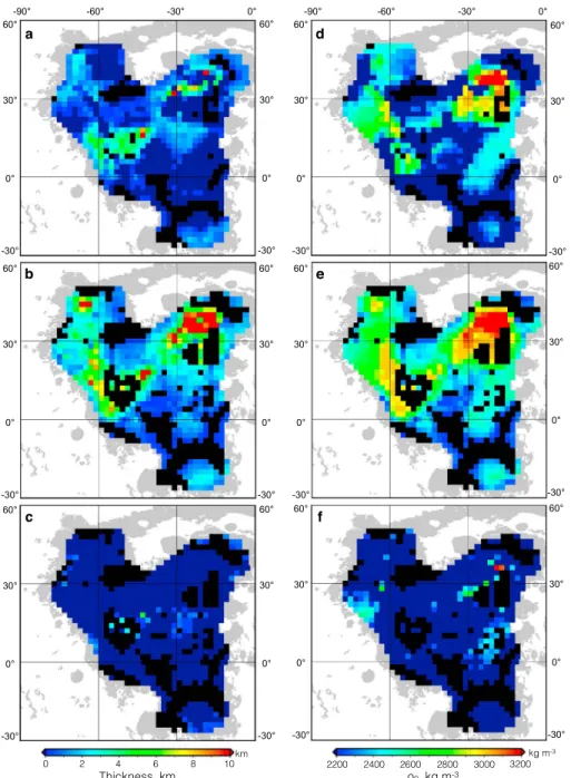
Figure 9. (a–c) Basalt thickness and (d–f ) upper crustal density using localization windows with𝜃₀= 8∘. (a) Best fit mare basalt thicknesses and (b) corresponding 1𝜎upper and (c) lower bounds. (d) Best fit uppermost highlands crustal densities and (e) corresponding 1𝜎upper and (f ) lower bounds. With a spectral bandwidth of 69, 10 windows with a concentration factor greater than 0.99 were used.

previous studies have suggested the basalt layer is thin, the Marius Hills region, within which lies the Marius Hills, a prominent long-lived volcanic center within Oceanus Procellarum [e.g., Whitford-Stark and Head, 1977, 1980; Hiesinger et al., 2011; Kiefer, 2013], and Mare Imbrium, where the crust is thin and an impact melt sheet might be present. After calculating the best fit parameters using a grid search method, the uncertainties of the inversion parameters were calculated using Monte Carlo simulations, as described in section 2. Given that it was numerically prohibitive to perform a Monte Carlo simulation for each analysis region, we performed such analyses only for eight different regions. The 1 and 2𝜎 limits were found to be very similar for each of these regions, and we thus adopted the average values of 0.1947 and 0.3529 for the 1 and 2𝜎 confidence intervals of𝜒2

r, respectively. Figure 6 plots the misfit as a function of the two inversion parameters for the same regions

Figure 10. Same as for Figure 9, but using localization windows with𝜃₀= 20∘. For this sized window, and with a spectral bandwidth of 58, there are 65 windows that possess concentration factors greater than 0.99.

the lower bound of the basalt thickness often corresponds to 0 km, and in some cases, the lower bound of the density of the underlying highlands corresponds to the minimum value used in our parameter search. A summary of the inversion results plotted in Figures 5 and 6 is provided in Table 1.

Figure 7 shows the spatial distribution of the best fit mare basalt thicknesses Tb(Figure 7a) with 1𝜎 lower

(Figure 7b) and upper (Figure 7c) bounds. In those regions where the 1𝜎 lower bound was not constrained, the bounding value of zero was plotted. In some places the best fitting model poorly fits the observations (plotted in black), and we only plot results when the minimum𝜒2

r misfit lies within the expected 2𝜎

confi-dence limit of 0.3529. The best fit thicknesses are found to lie in the range of 0 to 3.9 km. Excluding a few outliers, the average thickness is close to 1 km for most of Oceanus Procellarum and Mare Imbrium. The one major exception is for the region of Marius Hills in western Oceanus Procellarum where the thicknesses are considerably larger, close to 2.9 km. The uncertainties on these estimates are in general a couple of kilometers, and in many places the basalt thicknesses are compatible with being zero. Nevertheless, a few regions have

well defined 1𝜎 lower bounds on basalt thickness, including the region of Marius Hills whose lower bound is about 1 km. The 1𝜎 upper bounds are better defined, and as shown in Figure 7c, most of the mare basalts are no more than 3 km thick. The major exception is again the Marius Hills region, where the thickness could be up to 4.5 km. In the Imbrium basin, where previous gravity modeling has revealed a thin crust [see Wieczorek et al., 2013], the maximum basalt thickness is about 6 km.

Figure 8 illustrates the spatial distribution of the best fit upper crustal density𝜌₀(Figure 8a) with 1𝜎 lower (Figure 8b) and upper bounds (Figure 8c). This parameter is not as well constrained as the basalt thickness and spans almost the entire range of the investigated parameter space (2200–3200 kg m−3_{). The lower bound}

is for the most part not constrained, with two small exceptions being in the westernmost portion of Ocean Procellarum and within the central portion of Mare Imbrium. In contrast, the upper bound for most of the mare has a well defined value of about 2700 kg m−3_{, whereas the upper bound for the central portion of Mare}

Imbrium exceeds 3000 kg m−3_.

The above results were obtained using localization windows with an angular radius of 14∘. We tested the sensitivity of our results to the size of the window by using both a smaller window of𝜃 = 8∘ and a larger window of𝜃 = 20∘. By decreasing the window size to 8∘ the best fitting model parameters were found not to change much (see Figure 9). Nevertheless, the smaller number of well-localized tapers (10, in comparison to our nominal number of 27) resulted in larger data misfits, approximately 4 times larger, and slightly more scatter in the best fit values. In particular, some of the best fitting basalt thicknesses and 1𝜎 uncertainties were found to be equal to the maximum value of 10 km in our parameter search. Increasing the window size from 14∘ to 20∘ provides a larger number of localization windows (65) and hence a smaller range of uncertainties (Figure 10). However, as a result of the larger window size, the anomalously thick basalts associated with the Marius Hills region (as found using the smaller windows) are barely visible.

We tested the sensitivity of our results to the degree range over which the misfit was calculated. By modifying the upper and lower bounds by 50 degrees, our results were found to change only insignificantly. The assumed value of porosity in the mare basalts, however, is an important factor that affects the estimated mare basalt thicknesses. In our nominal models presented above, we used a value of 6%, and we tested the sensitivity of our results by using a porosity twice as large. Twelve percent is comparable to the average value found for the highland crust by Wieczorek et al. [2013], and this is likely to represent a maximal value for the mare basalts, given that they formed initially with little porosity and that they have been affected by less impact bombardment than the highlands. By increasing the porosity from 6% to 12%, we found that the mare basalt thicknesses increased by a factor of 1.5. By decreasing the porosity from 6% to 3%, the thicknesses decreased by a factor of 0.85.

4. Discussion

4.1. Comparison of Basalt Thickness Estimates

As noted in the introduction, mare basalt thicknesses have been estimated previously by several different approaches. In the work of De Hon [1974, 1977, 1979], the basalts which erupted exterior to a crater lead to a reduction in the crater rim height with respect to the crater surroundings. By the use of an empirical model of the rim height as a function of crater diameter for fresh craters, this allows the basalt thickness to be determined. It was found that the basalt thicknesses were on average about 400 m thick throughout much of Oceanus Procellarum. Locally, the thicknesses approach 1 km in places, and in the region of Marius Hills, the centers of the impact basins Humorum and Imbrium, as well as in Mare Cognitum (10.5∘S, 22.3∘W), thicknesses were inferred to be even larger, though only lower bounds of 1.5 km were provided.

Our work shows that the average thickness of basalts in northern Oceanus Procellarum (north of the equator) is about 0.80+1.02

−0.69km, which is about 2 times as large as the estimate from De Hon. We find the mare to be

thickest near Marius Hills, consistent with De Hon, but our estimates are about 2.9 times thicker. We find the basalts in southern Oceanus Procellarum to be thinner, on average about 0.14+0.36

−0.12km, and in many places

they are consistent with being zero. Our method does not provide estimates for basalt thicknesses in Mare Humorum. Though the basalt thicknesses are not well constrained in Mare Imbrium, our upper bound of about 2.45 km is consistent with De Hon’s lower bound.

The method used by De Hon only provides lower bounds on the basalt thicknesses, as only the basalts that erupted after the crater formed are measured. Thus, our estimates which are in general larger by almost a factor of 2 are not contradictory. Given that our approach has a very low spatial resolution, as a result of

the large size of the localization windows employed, it is not possible to compare thicknesses at specific locales. The only major inconsistency with De Hon is that we do not find evidence for thick basalt deposits in Mare Cognitum.

A different technique for estimating basalt thicknesses is to use the composition of a crater’s ejecta deposit as an indicator of whether the highlands underlying the basalts were excavated. These techniques provide basalt thicknesses that are somewhat greater (by about 500 m to 1 km) than those estimated by De Hon. Budney and Lucey [1998] investigated Mare Humorum, but because of the relatively small size of this basin (in comparison to our window size), our technique did not provide any results for this region. Heather and Dunkin [2002] investigated the southwestern region of Oceanus Procellarum, but for the most part only pro-vided lower bounds of a few hundred meters that are consistent with our estimates. Lower bounds of about 1 km were provided in the region of Marius Hills, which again are consistent with our results. Thomson et al. [2009] investigated the region of Mare Imbrium and obtained estimates that were about 0.5 km thicker than those of De Hon.

Radar sounding has also been used to estimate the thickness of mare basalts. This technique relies upon the assumption that the deepest subsurface reflector corresponds to the interface between the mare and high-lands. This assumption is difficult to assess, and furthermore, results from the Kaguya Lunar Radar Sounder [Ono et al., 2009; Pommerol et al., 2010; Oshigami et al., 2014] and Apollo Lunar Sounder Experiment [Peeples et al., 1978; Cooper et al., 1994] are not always concordant. The Apollo Lunar Sounder Experiment found evi-dence of a subsurface reflector along the equatorial ground track that was about 1 km deep in western Oceanus Procellarum, decreasing in depth eastward to about 400 m near the crater Kepler (8.1∘N, 38.0∘W). These estimates are broadly consistent with our estimates of about 1.06+0.87

−1.01km for this region, though it

is difficult to compare the single ground track with our results which have a much lower horizontal spatial resolution. The Kaguya radar sounder appears to provide thinner estimates than the Apollo radar sounder [Ono et al., 2009], and the origin of this discrepancy is not yet known.

Another method that has been used to constrain the thickness of mare basalts is based on the gravity signa-ture of buried impact craters. First, by detecting circular gravity anomalies that lack topographic expression, the diameter of the crater and its initial rim height can be estimated. If the crater was initially fresh and not degraded, the estimated rim height with respect to the surroundings would place a lower bound on the mare fill. Evans et al. [2016] obtained an average minimum bound of about 1.5 km, which is on the high end of our estimates, but within our 1𝜎 uncertainties. If, however, the crater rim was partially eroded prior to mare flood-ing, the minimum thicknesses would be even smaller. Second, some large craters likely excavated through the entire mare fill and into the underlying highland crust. By forward modeling the gravity signature of these craters, the total preimpact mare thickness is constrained to be less than about 7 km, which is again consistent with our results.

4.2. Marius Hills

Oceanus Procellarum is the largest contiguous expanse of lava flows on the Moon, spanning more than 2500 km from north to south, and comprising more than 50% of the Moon’s lava flows by area. Based on our analysis, the average thickness of these basalts is about 0.97+0.83

−0.85km. Marius Hills (∼200 × 250 km2area) is

one of the most prominent volcanic complexes within Oceanus Procellarum [Whitford-Stark and Head, 1977]. One of the oldest volcanic dome and cone complexes on the Moon, it stands about 0.5 km above the sur-rounding maria, contains over 250 small volcanic cones and domes, has two gravity anomalies suggestive of intrusions [Kiefer, 2013], and is floored by younger lavas that collect in the central part of Oceanus Procellarum [Whitford-Stark and Head, 1980; Hiesinger et al., 2011]. The region has two substantial Bouguer anomalies that Kiefer [2013] interpreted as representing important magmatic intrusions. Modeling these Bouguer anomalies as basaltic intrusions into a feldspathic crust implies thicknesses of at least 3 and 6.2 km for the two anomalies. In our study, we find that the Marius Hills themselves are associated with the central part of the broad area of maximum mare basalt thickness in central Oceanus Procellarum. The average thickness is about 2.86+0.79

−1.84km,

with the thickest part reaching up to 3.93+0.66

−1.39km. These results are consistent with the hypothesis that the

Marius Hills is a shield volcano [Spudis et al., 2013]. The results of Kiefer [2013] support this interpretation by showing that not only did large quantities of lava erupt effusively on the surface but also that large quantities of intrusive materials are also located within the crust.

4.3. Mare Imbrium

The Imbrium basin is one of the largest impact basins on the Moon, having formed around 3.85 Ga. With a radius of 1146 km, Mare Imbrium fills the interior of this basin and is the second largest mare, next to Oceanus Procellarum. Previous studies have suggested that the mare might be thicker than about 2.0 km in the central portion of the basin based on flooded crater studies and analysis of the ejecta of superposed impact craters. The thicknesses from our study are somewhat uncertain, possessing a range from 0.20 to 2.45 km. Though the best fit thicknesses are on the low side (∼0.87 km), the 1𝜎 upper bounds on the thickness (2.45 km) are among the thickest in our study.

As shown in Figure 8, the crust underlying the mare basalts is atypically dense in the central portion of Mare Imbrium. Whereas the density varies between 2200 kg m−3_{and 2800 kg m}−3_{elsewhere for most regions of}

Oceanus Procellarum, it reaches values up to 3100 kg m−3_{in the center of Mare Imbrium. This region of high}

density is located in that portion of the basin where the crust is predicted to be thin (∼10 km thick) [Wieczorek et al., 2013]. A plausible origin for the higher than typical crustal densities we find is that they are the result of a thick impact melt sheet that formed at the time of the Imbrium impact [e.g., Vaughan et al., 2013]. The composition of the Imbrium impact melts sampled exterior to the central portion of the basin are atypically mafic when compared to the feldspathic nature of the lunar crust [e.g., Ryder and Wood, 1977; Korotev, 2000], which would give them a higher than average intrinsic density. Furthermore, as this unit would have formed initially with zero porosity, it would naturally be more dense than the surrounding country rock. The result from sample analyses also show that the measured grain densities for Apollo impact melt breccias, dominated by Imbrium material, could range up to 3100 kg m−3_{[Kiefer et al., 2015], which is in agreement with our results.}

5. Conclusion

We use a multitaper spectral analysis of the Moon’s gravity and topography to constrain the density profile beneath the nearside mare. The high spectral bandwidths that are required for the localization windows are made possible by the high-resolution gravity data obtained by GRAIL. Our results show that with a poros-ity of 6%, the thickness of western mare basalts is 0.74+0.88

−0.64km, and the density of underlying upper crust

is 2335+151 −103kg m

−3_{. The mare basalts are thickest in central Oceanus Procellarum, with thicknesses up to}

2.86+0.79

−1.84km, centered on the Marius Hills, a prominent long-lived volcanic complex. Comparing with former

results based on flooded craters, our basalt thickness estimates are generally higher by a factor of about 2. Basalt thicknesses based on flooded craters are known to represent lower bounds, as the method is insensi-tive to the presence of mare basalts that erupted before the impact crater formed. In contrast, our results are generally concordant with studies that utilized the composition of a crater’s ejecta deposit to determine the total thickness of basalts.

References

Antonenko, I., and J. W. Head (1995), Estimates of cryptomare thickness and volume in Schiller-Schickard, Mare Humorum and Oceanus Procellarum areas, Proc. Lunar Planet. Sci. Conf., 26, 47–48.

Baldwin, R. B. (1949), The Face of the Moon, Univ. of Chicago Press, p. 239, Chicago, Ill. Baldwin, R. B. (1963), The Measure of the Moon, Univ. of Chicago Press, p. 488, Chicago, Ill.

Besserer, J., F. Nimmo, M. A. Wieczorek, R. C. Weber, W. S. Kiefer, P. J. McGovern, J. C. Andrews-Hanna, D. E. Smith, and M. T. Zuber (2014), GRAIL gravity constraints on the vertical and lateral density structure of the lunar crust, Geophys. Res. Lett., 41, 5771–5777, doi:10.1002/2014GL060240.

Braden, S. E., J. Stopar, M. S. Robinson, S. J. Lawrence, C. H. Van Der Bogert, and H. Hiesinger (2014), Evidence for basaltic volcanism on the Moon within the past 100 million years, Nat. Geosci., 7, 787–791, doi:10.1038/ngeo2252.

Budney, C. J., and P. G. Lucey (1998), Basalt thickness in Mare Humorum: The crater excavation method, J. Geophys. Res., 103(E7), 16,855–16,870, doi:10.1029/98JE01602.

Cooper, B. L., J. L. Carter, and C. A. Sapp (1994), New evidence for graben origin of Oceanus Procellarum from lunar sounder optical imagery,

J. Geophys. Res., 99(E2), 3799–3812, doi:10.1029/93JE03096.

De Hon, R. A. (1974), Thickness of mare material in the Tranquillitatis and Nectaris basins, in Proceedings of 5th Lunar Science Conference, vol. 5, pp. 53–59, Pergamon Press, New York.

De Hon, R. A. (1977), Mare Humorum and mare Nubium: Basalt thickness and basin-forming history, in Proceedings of the 8th Lunar Science

Conference, vol. 8, pp. 633–641, NASA, Houston, Tex.

De Hon, R. A. (1979), Thickness of the western mare basalt, in Proceedings of the 10th Lunar and Planetary Science Conference, pp. 2935–2955, Pergamon Press, New York.

De Hon, R. A., and J. D. Waskom (1976), Geologic structure of the eastern mare basins, in Proceedings of the 7th Lunar Science Conference, vol. 7, pp. 2729–2746, Pergamon Press, New York.

Eggleton, R. E., G. G. Schaber, and R. J. Pike (1974), Photogeologic detection of surfaces buried by mare basalts, Proc. Lunar Planet. Sci. Conf.,

5, 200–202.

Evans, A. J., J. M. Soderblom, J. C. Andrews-Hanna, S. C. Solomon, and M. T. Zuber (2016), Identification of buried lunar impact craters from GRAIL data and implications for the Nearside Maria, Geophys. Res. Lett., 43, 2445–2455, doi:10.1002/2015GL067394.

Acknowledgments

The GRAIL mission is supported by NASA’s Discovery Program and is performed under contract to the Massachusetts Institute of Technology and the Jet Propulsion Laboratory. M.W. and S.G. were supported by a grant from the French Space Agency (CNES) and S.G. was further supported by the National Natural Science Foundation of China

(11373058/11133004) and a China Scholarship Council doctoral fellowship. Data used to generate the results are available at http://pds-geosciences.wustl.edu and http://www.ipgp.fr/˜wieczor/.

Gillis, J. J., and P. D. Spudis (2000), Geology of the Smythii and Marginis region of the Moon: Using integrated remotely sensed data,

J. Geophys. Res. Planets, 105(E2), 4217–4233, doi:10.1029/1999JE001111.

Head, J. W. (1976), Lunar volcanism in space and time, Rev. Geophys., 14(2), 265–300, doi:10.1029/RG014i002p00265.

Head, J. W. (1982), Lava flooding of ancient planetary crusts: Geometry, thickness, and volumes of flooded lunar impact basins, Moon

Planets, 26(1), 61–88, doi:10.1007/BF00941369.

Head, J. W., and L. Wilson (1992), Lunar mare volcanism: Stratigraphy, eruption conditions, and the evolution of secondary crusts, Geochim.

Cosmochimi. Ac., 56(6), 2155–2175, doi:10.1016/0016-7037(92)90183-J.

Heather, D. J., and S. K. Dunkin (2002), A stratigraphic study of southern Oceanus Procellarum using Clementine multispectral data, Planet.

Space Sci., 50(14), 1299–1309, doi:10.1016/S0032-0633(02)00124-1.

Hess, P. C., and E. M. Parmentier (1995), A model for the thermal and chemical evolution of the Moon’s interior: Implications for the onset of mare volcanism, Earth Planet. Sci. Lett., 134(3), 501–514, doi:10.1016/0012-821X(95)00138-3.

Hess, P. C., E. M. Parmentier, and 0.-2. 28 032 (2001), Thermal evolution of a thicker KREEP liquid layer, J. Geophys. Res., 106(E11), doi:10.1029/2000JE001416.

Hiesinger, H., J. Head, U. Wolf, R. Jaumann, and G. Neukum (2011), Ages and stratigraphy of lunar mare basalts: A synthesis, Geol. Soc. Spec.

Pap., 477, 1–51.

Hörz, F. (1978), How thick are lunar mare basalts, in Proceedings of the 9th Lunar and Planetary Science Conference, pp. 3311–3331, NASA, Houston, Tex.

Huang, Q., and M. A. Wieczorek (2012), Density and porosity of the lunar crust from gravity and topography, J. Geophys. Res., 117, E05003, doi:10.1029/2012JE004062.

Kiefer, W. S. (2013), Gravity constraints on the subsurface structure of the Marius Hills: The magmatic plumbing of the largest lunar volcanic dome complex, J. Geophys. Res. Planets, 118, 733–745, doi:10.1029/2012JE004111.

Kiefer, W. S., R. J. Macke, D. T. Britt, A. J. Irving, and G. J. Consolmagno (2012), The density and porosity of lunar rocks, Geophys. Res. Lett., 39, L07201, doi:10.1029/2012GL051319.

Kiefer, W. S., R. J. Macke, D. T. Britt, A. J. Irving, and G. J. Consolmagno (2015), The density and porosity of lunar impact breccias and impact melt rocks and implications for gravity modeling of impact basin structure, in Early Solar System Impact Bombardment III, p. 3004, LPI Contributions No. 1826, Houston, Tex.

Konrad, W., and T. Spohn (1997), Thermal history of the Moon: Implications for an early core dynamo and post-accertional magmatism,

Adv. Space Res., 19(10), 1511–1521, doi:10.1016/S0273-1177(97)00364-5.

Korotev, R. L. (2000), The great lunar hot spot and the composition and origin of the Apollo mafic (“LKFM”) impact-melt breccias, J. Geophys.

Res., 105(E2), 4317–4345, doi:10.1029/1999JE001063.

Laneuville, M., M. A. Wieczorek, D. Breuer, and N. Tosi (2013), Asymmetric thermal evolution of the Moon, J. Geophys. Res. Planets, 118, 1435–1452, doi:10.1002/jgre.20103.

Lemoine, F. G., et al. (2014), GRGM900C: A degree 900 lunar gravity model from GRAIL primary and extended mission data, Geophys. Res.

Lett., 41, 3382–3389, doi:10.1002/2014GL060027.

Ono, T., A. Kumamoto, H. Nakagawa, Y. Yamaguchi, S. Oshigami, A. Yamaji, T. Kobayashi, Y. Kasahara, and H. Oya (2009), Lunar Radar Sounder observations of subsurface layers under the nearside maria of the Moon, Science, 323(5916), 909–912, doi:10.1126/science.1165988. Oshigami, S., S. Watanabe, Y. Yamaguchi, A. Yamaji, T. Kobayashi, A. Kumamoto, K. Ishiyama, and T. Ono (2014), Mare volcanism:

Reinterpre-tation based on Kaguya Lunar Radar Sounder data, J. Geophys. Res. Planets, 119, 1037–1045, doi:10.1002/2013JE004568.

Papike, J. J., G. Ryder, and C. K. Shearer (1998), Lunar samples, in Planetary Materails, vol. 36, chap. 5, pp. 5–1–5-234, Mineralog. Soc. of Am., Washington, D. C.

Peeples, W. J., W. R. Sill, T. W. May, S. H. Ward, R. J. Phillips, R. L. Jordan, E. A. Abbott, and T. J. Killpack (1978), Orbital radar evidence for lunar subsurface layering in Maria Serenitatis and Crisium, J. Geophys. Res., 83(B7), 3459–3468, doi:10.1029/JB083iB07p03459.

Pérez-Gussinyé, M., A. R. Lowry, A. B. Watts, and I. Velicogna (2004), On the recovery of effective elastic thickness using spectral methods: Examples from synthetic data and from the Fennoscandian Shield, J. Geophys. Res., 109, B10409, doi:10.1029/2003JB002788. Pike, R. J. (1967), Schroeter’s rule and the modification of lunar crater impact morphology, J. Geophys. Res., 72(8), 2099–2106,

doi:10.1029/JZ072i008p02099.

Pike, R. J. (1972), Geometric similitude of lunar and terrestrial craters, in 24th International Geological Congress, vol. 15, pp. 41–47, NASA, Montreal, Canada.

Pommerol, A., W. Kofman, J. Audouard, C. Grima, P. Beck, J. Mouginot, A. Herique, A. Kumamoto, T. Kobayashi, and T. Ono (2010), Detectability of subsurface interfaces in lunar maria by the LRS/SELENE sounding radar: Influence of mineralogical composition,

Geophys. Res. Lett., 37, L03201, doi:10.1029/2009GL041681.

Prettyman, T. H., J. J. Hagerty, R. C. Elphic, W. C. Feldman, D. J. Lawrence, G. W. McKinney, and D. T. Vaniman (2006), Elemental composition of the lunar surface: Analysis of gamma ray spectroscopy data from Lunar Prospector, J. Geophys. Res., 111, E12007, doi:10.1029/2005JE002656.

Ryder, G., and J. A. Wood (1977), Serenitatis and Imbrium impact melts: Implications for large-scale layering in the lunar crust, in Proceedings

of the 8th Lunar Science Conference, pp. 655–668, Pergamon Press, New York.

Shearer, C. K., et al. (2006), Thermal and magmatic evolution of the Moon, Rev. Miner. Geochem., 60(1), 365–518, doi:10.2138/rmg.2006.60.4. Smith, D. E., et al. (2010), Initial observations from the Lunar Orbiter Laser Altimeter (LOLA), Geophys. Res. Lett., 37, L18204,

doi:10.1029/2010GL043751.

Solomon, S. C., and J. W. Head (1980), Lunar mascon basins: Lava filling, tectonics, and evolution of the lithosphere, Rev. Geophys., 18(1), 107–141, doi:10.1029/RG018i001p00107.

Spohn, T., W. Konrad, D. Breuer, and R. Ziethe (2001), The longevity of lunar volcanism: Implications of thermal evolution calculations with 2D and 3D mantle convection models, Icarus, 149(1), 54–65, doi:10.1006/icar.2000.6514.

Spudis, P. D., P. J. McGovern, and W. S. Kiefer (2013), Large shield volcanoes on the Moon, J. Geophys. Res. Planets, 118, 1063–1081, doi:10.1002/jgre.20059.

Thomson, B. J., E. B. Grosfils, D. B. J. Bussey, and P. D. Spudis (2009), A new technique for estimating the thickness of mare basalts in Imbrium Basin, Geophys. Res. Lett., 36, L12201, doi:10.1029/2009GL037600.

Vaughan, W. M., J. W. Head, L. Wilson, and P. C. Hess (2013), Geology and petrology of enormous volumes of impact melt on the Moon: A case study of the Orientale basin impact melt sea, Icarus, 223(2), 749–765, doi:10.1016/j.icarus.2013.01.017.

Whitford-Stark, J. L., and J. W. Head (1977), The Procellarum volcanic complexes: Contrasting styles of volcanism, in Proceedings of the 8th

Lunar Science Conference, pp. 2705–2724, Pergamon Press, New York.

Whitford-Stark, J. L., and J. W. Head (1980), Stratigraphy of Oceanus Procellarum basalts: Sources and styles of emplacement, J. Geophys.

Wieczorek, M. A. (2015), Gravity and topography of the terrestrial planets, in Treatise on Geophysics, 2nd ed., edited by G. Schubert, pp. 153–193, Elsevier, Oxford, doi:10.1016/B978-0-444-53802-4.00169-X.

Wieczorek, M. A., and R. J. Phillips (1998), Potential anomalies on a sphere: Applications to the thickness of the lunar crust, J. Geophys. Res.,

103, 1715–1724, doi:10.1029/97JE03136.

Wieczorek, M. A., and R. J. Phillips (2000), The “Procellarum KREEP Terrane”: Implications for mare volcanism and lunar evolution, J. Geophys.

Res., 105(E8), 20,417–20,430, doi:10.1029/1999JE001092.

Wieczorek, M. A., and F. J. Simons (2005), Localized spectral analysis on the sphere, Geophys. J. Int., 162(3), 655–675, doi:10.1111/j.1365-246X.2005.02687.x.

Wieczorek, M. A., and F. J. Simons (2007), Minimum-variance multitaper spectral estimation on the sphere, J. Fourier Anal. Appl., 13(6), 665–692, doi:10.1007/s00041-006-6904-1.

Wieczorek, M. A., M. T. Zuber, and R. J. Phillips (2001), The role of magma buoyancy on the eruption of lunar basalts, Earth Planet. Sci. Lett.,

185(1), 71–83, doi:10.1016/S0012-821X(00)00355-1.

Wieczorek, M. A., et al. (2013), The crust of the Moon as seen by GRAIL, Science, 339(6120), 671–675, doi:10.1126/science.1231530. Wieczorek, M. A., M. Meschede, and I. Oshchepkov (2015), SHTOOLS: Tools for working with spherical harmonics (v3.1), ZENODO,

doi:10.5281/zenodo.20920.

Yingst, R. A., and J. W. Head (1997), Volumes of lunar lava ponds in South Pole-Aitken and Orientale Basins: Implications for eruption conditions, transport mechanisms, and magma source regions, J. Geophys. Res., 102(E5), 10,909–10,931, doi:10.1029/97JE00717. Zuber, M. T., et al. (2013), Gravity field of the Moon from the Gravity Recovery And Interior Laboratory (GRAIL) mission, Science, 339(6120),