Evidence for precursor superconducting pairing above T c in underdoped cuprates from an analysis of the in-plane infrared response

This content has been downloaded from IOPscience. Please scroll down to see the full text.

Download details:

IP Address: 134.21.47.224

This content was downloaded on 18/09/2015 at 07:51

Please note that terms and conditions apply.

Evidence for precursor superconducting pairing above Tc in underdoped cuprates from an

analysis of the in-plane infrared response

View the table of contents for this issue, or go to the journal homepage for more 2015 New J. Phys. 17 053022

PAPER

Evidence for precursor superconducting pairing above

T

c

in

underdoped cuprates from an analysis of the in-plane infrared

response

B Šopík1 , J Chaloupka1 , A Dubroka1,2 , C Bernhard3 and D Munzar1,2

1 _{Central European Institute of Technology, Masaryk University, Kamenice 753/5, 62500 Brno, Czech Republic}

2 _{Department of Condensed Matter Physics, Faculty of Science, Masaryk University, Kotlářská 2, 61137 Brno, Czech Republic} 3 _{University of Fribourg, Department of Physics and Fribourg Centre for Nanomaterials, Chemin du Musée 3, CH-1700 Fribourg,}

Switzerland

E-mail:sopik@ceitec.muni.czandmunzar@physics.muni.cz

Keywords: cuprate superconductors, infrared response, precursor superconducting pairing above Tc

Abstract

We performed calculations of the in-plane infrared response of underdoped cuprate superconductors

to clarify the origin of a characteristic dip feature which occurs in the published experimental spectra

of the real part of the in-plane conductivity below an onset temperature T

ons

_{considerably higher than}

T

c

. We provide several arguments, based on a detailed comparison of our results with the published

experimental data, confirming that the dip feature and the related features of the memory function

ω

=

ω

+

ω

M

( )

M

1

( )

i

M

2

( )

(a peak in M

1

and a kink in M

2

) are due to superconducting pairing

correlations that develop below T

ons

_{. In particular, we show that (i) the dip feature, the peak and the}

kink of the low-temperature experimental data can be almost quantitatively reproduced by

calculations based on a model of a d-wave superconductor. The formation of the dip feature in the

experimental data below T

ons

_{is shown to be analogous to the one occurring in the model spetra below}

T

c

. (ii) Calculations based on simple models, for which the dip in the temperature range from

T

c

to

T

ons

_{is unrelated to superconducting pairing, predict a shift of the onset of the dip at the high-energy}

side upon entering the superconducting state, that is not observed in the experimental data; (iii) the

conductivity data in conjunction with the recent photoemission data (Reber et al 2012 Nat. Phys.

8

606

, Reber et al 2013 Phys. Rev. B

87 060506

) imply the persistence of the coherence factor

characteristic of superconducting pairing correlations in a range of temperatures above

T

c

.

1. Introduction

The possible persistence of some form of superconductivity, at least pairing correlations, many tens of K above the bulk superconducting transition temperatureTcin underdoped (UD) cuprate superconductors belongs to

the most vividly discussed topics in thefield of high-Tcsuperconductivity, for representative examples of related

experimental studies, see [1–15]. Surprisingly high (up to about 100 K aboveTc) values of the temperature Tons

of the onset of an increase of coherence, presumably due to an onset of precursor superconducting pairing correlations, have been deduced from the data of the c-axis infrared response of UD YBa2Cu3O7−δ(Y-123) [6].

More recently, the interpretation of the Tonsscale in terms of a precursor superconductivity has been supported by results obtained by Uykur and coworkers [7]. They address the persistence of the superfluid density aboveTc

and the impact of Zn doping on Tons_(Tp_{in the notation of [7]). This interpretation, however, has not yet been}

commonly accepted. Two reasons are: (i) the c-axis response of Y-123 is a fairly complex quantity due to the specific bilayer structure of this compound. Its interpretation therefore requires a detailed understanding of the c-axis electrodynamics of the bilayer compounds [16–23]. (ii) UD cuprates are known to exhibit ordered phases distinct from superconductivity, in particular, charge modulations have been reported [24,25], that set in at temperatures comparable to Tons_{. This has fueled speculations that the T}ons_{scale is determined by an order}

OPEN ACCESS

RECEIVED

17 December 2014

REVISED

31 March 2015

ACCEPTED FOR PUBLICATION

15 April 2015

PUBLISHED

15 May 2015

Content from this work may be used under the terms of theCreative Commons Attribution 3.0 licence.

Any further distribution of this work must maintain attribution to the author(s) and the title of the work, journal citation and DOI.

different from and possibly competing with superconductivity rather than by pairing correlations themselves. In this context, it is of high importance to identify manifestations of the increase of coherence below Tons_{in the}

in-plane response, a quantity revealing aspects of the electronic structure complementary to those manifesting themselves in the c-axis response, and to ascertain their relation to superconducting pairing correlations.

It has been already shown [6] that the real part of the in-plane infrared conductivity of UD Y-123 changes at

Tonsin a way similar to that of an optimally doped (OPD) superconductor atTc: a dip-like feature with a

minimum around_{400 cm}−1_{begins to form and this is accompanied by a pronounced spectral weight shift from}

the dip region to very low frequencies (below ca_{200 cm}−1_{). The focus, however, has been on qualitative aspects}

of the relevant spectral weight shifts, and the related spectral structures have not been addressed. Here we concentrate on three prominent spectral features that develop below Tons: the onset of the dip at the high energy side, the corresponding peak in the spectra of the real part of the memory function and the corresponding kink in the spectra of the imaginary part of the memory function. Our analysis involves comparisons of the data of two representative UD cuprates with those of OPD ones and with results of our calculations employing approaches ranging from the Allen’s theory to the fully selfconsistent generalized Eliashberg theory. It provides evidence that the features are due to superconducting pairing correlations, and the scale Tons_{due to a precursor}

superconducting pairing phase rather than to an ordered state unrelated to superconductivity.

Recall that Tonsis significantly lower than T*, the temperature of the onset of the pseudogap as seen, e.g., in the planar copper Knight shift [26], in the c-axis conductivity [27–30], in the intrinsic tunnelling [31,32], in the angular resolved photoemission spectra of the antinodal region of the Brillouin zone [33] etc. For UD Y-123 with 10% dopingT*>300 K [6,7,28,29,34], whileTons≈170 K_{[6,7]. The pseudogap region of the phase} diagram of the cuprates located between theTcline and the T* line involves two distinct types of electronic

correlations: the correlations setting on at T*, on the one hand, cause a depletion of the electronic density of states at low energies and they seem to compete with superconductivity [30]. The correlations setting on at Tons_,

on the other hand, bring about an increase of coherence of the electronic states manifesting themselves both in the out-of plane and in the in-plane response [6].

The paper is organized as follows. In section2we summarize the relevant aspects of the experimental infrared data. As examples we use the published data of UD HgBa2CuO4+δ(Hg-1201) [35] and Y-123 [6,36]. At

the end of the section, the data are compared with the published ones of OPD cuprates. In section3we present and discuss results of our calculations aiming to clarify the origin of the spectral structures. First (in

subsection3.1), we focus on the spectra calculated using the Eliashberg theory. We put emphasis on the similarity between the low-temperature (T) data and the low-T calculated spectra and on the similarity between the onset of the spectral structures below Tons_{in UD cuprates and that belowT}

cin the calculated spectra. In

subsection3.2, the data are discussed in terms of the frequently used extended Allen’s theory (EAT) [36–39]. It is highlighted that the assumption of a superconductivity unrelated gap in the density of states in the temperature rangeTc <T<Tonsleads to inconsistencies with the data. In particular, we show that it leads to a clear shift of

the high energy onset of the dip upon entering the superconducting state, that is not observed in the

experimental data. This applies also to simple models, where the dip in the temperature rangeTc< T< Tonsis

attributed solely to an electron–boson coupling and the temperature dependence of the Fermi and Bose factors. Finally, in subsection3.3, we present and discuss results of our calculations of the optical spectra, using as inputs recently published properties of the quasiparticle spectral function obtained from the photoemission data by means of analyzing the tomographic density of states [10]. A short summary and conclusions are given in section4.

2. Relevant aspects of the published experimental data

The dip feature in the spectra of the real part σ1of the infrared conductivityσ will be illustrated with the recently

published data of UD HgBa2CuO4+δ(Hg-1201) with 10% doping andTc =67 K[35]. Also discussed will be the

related structures of the memory functionM( )ω =M1( )ω +M2( )ω , defined by 

σ ω( )=iε ω0 pl2 [M( )ω +ω][40] and connected to the so called optical selfenergy∑opt( )ω by

ω ω

∑opt( )= −M( ) 2. Here ωplis the plasma frequency. The data of UD Hg-1201 of [35] are similar to the

earlier published ones of UD Y-123 [6,36], but a much more detailed temperature dependence is reported and some spectral features are sharper than in Y-123.

Figure1shows, in part (a), a selection of the spectra of σ1of Hg-1201 fromfigure 1 of [35], and, in parts (b)

and (c), the corresponding spectra of M1and M2fromfigure 4 of [35]. The low-temperature spectra of σ1

contain theδ-peak at ω = 0 (not shown in the figure) corresponding to the loss-free contribution of the superconducting condensate, a narrow low-energy component corresponding to residual quasiparticles, and a deep and broad minimum around 30 meV (see, e.g., the 10 K line infigure1(a)). This is followed by a broad region of an approximately linear increase terminating atEg≈140 meV, where the slope of the spectrum

changes, see the arrow infigures1(a) andfigure2. This change of slope will be called the high energy onset of the dip (HEOD). It is associated with a local maximum at a slightly higher energy. The HEOD is further

accompanied by a characteristic peak in the spectra of M1with an onset feature at the high energy side (around Eg), and a kink in those of M2, see the arrows infigures1(b) and (c). All the three features are well known from

earlier infrared studies [28,36,38,39,41]. What has, however,—to the best of our knowledge—not yet been recognized, is the fact that they start to form close to the temperature Tonsof [6].

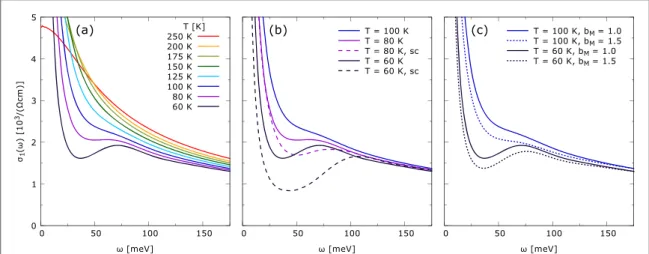
Figure 1. (a) Real part of the in-plane infrared conductivity of Hg-1201 with 10% doping andTc=67 Kforfive selected temperatures

(data obtained by Mirzaei and coworkers, published infigure 1 of [35]). (b), (c): the corresponding spectra of M1and M2, respectively

(data fromfigure 4 of [35]). The arrows indicate the features discussed in the text: the one in (a) the change of slope ofσ1, the left (right) one in (b) the maximum (the onset feature at the high energy side) of the characteristic peak of M1, and that in (c) indicates the

kink of M2. (d), (e), (f): The spectra ofσ1, M1and M2calculated using the model of charged quasiparticles coupled to spinfluctuations

and the fully selfconsistent generalized Eliashberg equations. (g), (h), (i): The normal (green) and superconducting state (violet) spectra ofσ1, M1and M2calculated using the hybrid approach. The dotted lines in (h) and (i) represent the derivatives of M1and M2.

They are shown to highlight the shift of the structures due toΔSC. The vertical lines are guides to the eye.

Figure 2. Real part of the in-plane infrared conductivity of Hg-1201 with 10% doping andTc=67 Kfor eight selected temperatures

(data obtained by Mirzaei and coworkers published in_{figure 1 of [}35]). The dotted lines represent linear extrapolations and are shown to highlight the high-energy onset of the dip discussed in the text.

This will be discussed below. We focus on σ1first. The70 Kand120 Kspectra infigure1(a) display a clear

HEOD at an energy close to Eg, see alsofigure2. The 250 K spectrum, on the other hand, does not display any

such feature in the relevant spectral range. It can be seen infigure 1 of [35], see alsofigure2, that the dip feature vanishes at a temperature higher than160 Kbut⩽200 K, close to the maximum Tonsof [6] (180 K). Based on thisfinding and the earlier observations of [6] we assume that the temperature scale of the dip coincides with the earlier established Tons_{of [6] and T}p

of [7] and denote it by Tons_{. The T-dependence of the characteristic peak in}

the spectra of M1is similar: at70 Kand120 Kit is still very pronounced and almost at the same location as at low

temperatures, at 250 K a clear maximum is not evident (see alsofigure 4 of [35]; the remaining very weak band in the 90–130 meVrange seems to be of different origin, perhaps related to the sharp structure at ca80 meV). Note that the onset feature at the high energy side of a similar peak occurring in the case of UD Y-123 has already been reported to vanish around170 K[36], see discussion offigure 7 in [36]. Next we address the T-dependence of the kink in the spectra of M2. At low temperatures the feature is very sharp (note that the 10 K spectrum

overshoots the70 Kone). It gets less sharp aroundTcbut persists, at approximately the same energy, up to much

higher temperatures, seefigure 4 of [35]. In the 120–200 Krange, it transforms into a smoother onset at a lower energy due to the presence of the relatively narrow low energy component of σ1, that can be seen infigure2,

rather than to the HEOD. Notefinally that the onset of the features is very likely connected with a transition to a purely quadratic T-dependence of the dc resistivity occurring slightly above 200 K [35] and with the appearance below about 200 K of a Fermi-liquid like scaling ofM ( ) [ω 35].

In OPD materials, a dip feature inσ ω1( )terminated by a local maximum, a peak inM ( )1 ω and a kink in

ω

M ( )2 , similar to those discussed above, set in atTc(or very slightly aboveTc). For representative examples, see

[42–45]. These features of OPD materials are clearly caused by superconductivity, since they develop in parallel with the formation of the loss-free contribution to σ ω( ) of the superconducting condensate, involving the δ-peak at ω = 0 inσ ω1( ): theδ-peak collects the spectral weight lost by the formation of the dip. It appears, that

the three features of OPD materials, that set in atTcand are due to superconductivity, continuously transform

into those of the UD ones, setting in at Tons. This is a strong phenomenological argument in favor of the superconducting pairing-based interpretation of the three features and the precursor superconducting pairing based interpretation of the Tons_scale.

3. Results and discussion

3.1. Response functions calculated using the Eliashberg theory, comparison with the data

Recall that many properties of OPD cuprate superconductors, including superconductivity, can be (at least qualitatively) understood in terms of (various versions of) the model, where charged planar quasiparticles are coupled to spinfluctuations. For reviews, see [46–51]. In particular, the low-T spectra of σ1in the

superconducting state have been well reproduced [52–55] using a phenomenological version of the model, where the spinfluctuation spectrumχ ν( , )q is approximated by a narrow (inν) mode centered at the frequency of the magnetic resonance. By including a continuum contribution toχ ν( , )q and performing the calculations at the fully selfconsistent generalized Eliashberg level, almost quantitative agreement with the data can be achieved [56], see also [57]. In the following we demonstrate that even the low-T experimental spectra of UD Hg-1201 can be approximately reproduced using the generalized Eliashberg approach formulated in [56]. In order to avoid any misunderstanding, we emphasize here that it is not the purpose of the present paper to advocate a very specific model. There are only two ingredients of the model, that are really essential for our conclusions: the superconducting order of d-wave symmetry and the relatively strong coupling between charge carriers and bosonic excitations (not necessarily spinfluctuations), whose spectral density is peaked around 40–50 meV. Other ingredients—the presence of a tail of the spectrum of the bosonic excitations ranging to high energies, the full selfconsistency etc.—help to reproduce the low temperature data quantitatively.

We begin with a brief description of the computational approach, details can be found in appendixA. The generalized Eliashberg equations (see, e.g., [58]) can be written as

∑

Σ ω β χ ν ω ν = − −

(

k

)

g_N

(

q

) (

G k q

)

ˆ i ,n i , ˆ i i , , (1) m m n m q 2 ,

where Σˆ is the matrix selfenergy that can be expressed in terms of the Pauli matrices as

Σˆ =Σ(0)τˆ +Σ τˆ +Σ τˆ

0 (3) 3 (1) 1,Gˆ= G(0)τˆ0+G(3)τˆ3+G(1)τˆ1is the renormalized quasiparticle propagator,

ω = ω τ − ϵ −μ τ −Σ ω −

(

)

(

)

Gˆ i n,k i nˆ [ ( )k ] ˆ ˆ i ,n k , (2) 1 0 3

χ ν(i , )m q is the Matsubara counterpart of the the spin susceptibility, g is the coupling constant,iωnandiνmare

the fermionic and bosonic Matsubara energies, respectively. The equations have been solved on the real axis using spectral representations of Gˆ andχ. We have used the same form of the input spin susceptibility as in our

previous studies [55] and [56]. It contains a narrow (in frequency) mode centered at the frequency of the magnetic resonance and a component approximating the spin-fluctuation continuum. The corresponding formulas, the values of all input parameters, providing the values ofTcandΔmaxof133 Kand45 meV,

respectively, and some intermediate results are given in appendixA. HereΔ_maxis the maximum value of the superconducting gap ofdx2−y2symmetry. The high value ofT_cis not surprising considering the observation of

[59] that the value of the spin-fermion coupling constant providing the bestfit of the nodal kink in UD Y-123 yields a highTcvalue of175 K.

Finally, after obtaining the selfconsistent solution of the generalized Eliashberg equations, the optical conductivity was calculated using the formula

 σ ω Π ω ω = − + + N d K ( ) ie ( ) i0 . (3) xx p xx xx 2 ⎡⎣ ⎤⎦

Here d is the c-axis lattice parameter (d = 9.52 Å for Hg-1201, d = 11.65 Å for Y-123), Npis the number of CuO2

planes within a unit cell (Np= 1 for Hg-1201, Np= 2 for Y-123) andω is here in units of energy. The expressions

Kxxand Πxx( )ω in the numerator provide the diamagnetic and paramagnetic contributions to the optical

conductivity, respectively. Both can be expressed in terms of the matrix quasiparticle spectral function

τ τ τ

= + +

Aˆ A(0)ˆ A ˆ A ˆ

0 (3) 3 (1) 1defined byAˆ ( , )ω k = −2 Im{ ˆ (G ω+i0, )}. The diamagnetic term is given byk

the following formula (exact)

∫

∑

ϵ π β = − ∂ ∂ − −∞ ∞

( )

K N _{k a} E A E E k k 1 ( ) 1 d 2 ( , )tanh 2 . (4) xx x k 2 2 (3) ⎡ ⎣⎢ ⎤ ⎦⎥

The paramagnetic term is given by the current–current correlation function and can be expressed (in terms of

Aˆ) only approximately. The most frequently used approximation, employed also in our calculations, completely neglects vertex corrections and leads to the following formula for the imaginary part Π″xxofΠxx:

∫

∑

Π ω ϵ ν π ν ν ω ν ν ω ″ = − ∂ ∂ × + − + −∞ ∞

{

}

N k a A A k k k ( ) 1 2 ( ) d 2 Tr ˆ ( , ) ˆ ( , ) [f( ) f( )]. (5) xx x k 2 ⎛ ⎝ ⎜ ⎞ ⎠ ⎟

The real part Π′_xxofΠ_xxwas obtained using the Kramers–Kronig transformation. Note that the expression on

the right hand side of equation (3) includes the contribution of the condensate, the superfluid plasma energy ω_pl,scis given by  ω ϵ Π = N ′ − d K e (0) . (6) p xx xx 2 pl,sc2 2 0 ⎡⎣ ⎤⎦

In order to assess the validity of the approximation of equation (5), we have also evaluatedΠ_xxusing the gauge invariant approach of [56], where an important class of vertex corrections is included. The corrections modify the spectra of Π″_xxonly slightly, the only significant problem of the approximation being an

underestimation of the total spectral weight atfinite frequencies and Π∣ ′xx(0)∣by ca 8%. For the normal state, this leads to the presence of a small unphysical singular component. In order to avoid the problem, we have replaced Kxxwith Π′ (0)xx in the normal state calculations. For temperatures belowTc, we have setKxx=Πxx′ (0)[140 K].

The corresponding value of the (total) plasma energyωplis1.95 eV.

For future reference, we provide here also the formula for the real partσ ω1( )of σxx( )ω resulting from

equation (5): 

∑

∫

σ ω ω ϵ ν π ν ν ω ν ν ω ν ν ω = ∂ ∂ + + + − + −∞ ∞

}

( )

N d N k a A A A A k k k k ( ) e 1 d 2 { ( , ) ( , ) ( , ) ( , ) [f( ) f( )], (7) p x k 1 2 2 (1) (1) ⎛ ⎝ ⎜ ⎜ ⎞ ⎠ ⎟ ⎟

whereA( , )ν k =A(0)( , )ν k +A(3)( , )ν k is the usual spectral function. The normal state version of the formula reads



∫

∑

σ ω ω ϵ ν π ν ν ω ν ν ω = ∂ ∂ × + − + −∞ ∞

( )

N d N k a A k A k ( ) e 1 d 2 ( , ) ( , )[f( ) f( )]. (8) p x k 1 2 ⎛ 2 ⎝ ⎜ ⎜ ⎞ ⎠ ⎟ ⎟

Figures1(d)–(f) show the calculated spectra of σ1, M1, and M2, respectively. Note the agreement between the

low-T spectra and the low-T data shown infigures1(a)–(c). The structures of σ1and M2, in particular a weak

onset around the energy of the resonance modeω0(here 50 meV), and the HEOD of σ1and the corresponding

kink of M2at≈ω0+2Δmax, can be interpreted along the lines of the earlier theoretical studies [55,56]. For the

convenience of the reader, the interpretation is summarized in the following paragraph.

Figure3(a) shows the30 Kspectra of σ1and M2fromfigures1(d) and (f) and the corresponding spectra of

the second derivative of ωM2, all in arbitrary units. The arrows indicate three important features, occuring also

in the experimental spectra of OPD cuprates, whose interpretation was presented in [55,56]: (i) a weak onset of

σ1and M2around the energyω0of the bosonic mode (within the present context the magnetic resonance)

[43,44,52,55,56]. (ii) A maximum of the second derivative of ωM2[60] at approximatelyω0+ Δmax

[53,55,56]. (iii) A local maximum of σ1at Egwith Egapproximately equal or slightly aboveω0+2Δmax

[43,44,54,56], associated with the HEOD, and the corresponding kink of M2. At the simplest relevant

perturbative level (Bogolyubov quasiparticles of a d-wave superconductor coupled to bosons), the basic infrared activefinal states consist of two Bogolyubov quasiparticles and the bosonic mode, see figure3(b). Final states consisting of two Bogolyubov quasiparticles are not infrared active in the clean limit. The features (i), (ii), and (iii) are due, as detailed in [55,56], to the appearance above the characteristic energies (ω0,ω0+ Δmax,

ω0+ 2Δmax) offinal states consisting of (i) two near nodal (Bogolyubov) quasiparticles and the bosonic mode,

(ii) a near nodal quasiparticle, an antinodal quasiparticle and the mode, and (iii) two antinodal quasiparticles and the mode. Aboveω0+ 2Δmax, the density of availablefinal states saturates. A schematic representation of

the three types offinal states, associated with the features (i), (ii), and (iii) is presented in figure3(c).

The relationEg≈ 2Δmax + ω0[54–56] allows for a quantitative consistency check. The value of Egof UD

Hg-1201 of140 meVis indeed approximately consistent with the available experimental values ofω0andΔmax

(ω ≈0 50 meV[61], Δmax ≈ 39 meV[62], Δmax ≈45 meV[63]). Recently, a similar consistency check has

been applied to the infrared data of OPD Bi2Sr2CaCu2O8+δ(Bi-2212) by Homes and coworkers [64]. To

conclude, the low-T infrared spectra of UD Hg-1201are consistent with a well established model of a d-wave superconductor.

Next we address the T-dependence of the model spectra. It can be seen infigures1(d)–(f) that the three

important features (the dip of σ1, the maximum of M1and the M2kink) develop belowTcin the same fashion as

in the data of OPD materials [42–45]. In particular, the σ1dip forms already close toTc. What we would like to

highlight here is that not only the T dependence of the data of OPD cuprates but also that of the UD is similar to the model spectra, comparefigures1(a)–(c) with figures1(d)–(f). Note that the development of the dip in the UD Hg-1201 belowTons≈ 180 K_{is analogous to that of the model spectra belowT}

c: somewhat below Tons/Tca

characteristic change of slope appears inσ ω1( ), with decreasing T its energy approaches Egand the minimum at

low energies and the characteristic maximum around Egare forming. In the model spectra, the energy scale of

Figure 3. (a) 30 K spectra ofσ1and M2fromfigure1(d), (f) and the corresponding spectra of the second derivative ofωM2, all in arbitrary units. The arrows indicate three important features discussed in the text. (b) Diagrammatic representation of thefinal states discussed in the text. The solid lines denote Bogolyubov quasiparticles, the dashed line a boson participating in thefinal state, within the present scheme the resonance. (c) Schematic representation of the three types offinal states associated with the features (i), (ii), (iii). We show thefirst Brillouin zone and the Fermi surface, the symbols represent the Bogolyubov quasiparticles, the arrows the

the dip develops more gradually than in the data. This difference is most likely due to the meanfield character of the model. The similarity between the T-dependence of the data below Tons_{and that of the model spectra below}

Tcprovides a further support for the interpretation of the Tonsscale in terms of a precursor superconducting

pairing state, for which Tonscorresponds to the meanfield transition temperature.

Admittedly, the meanfield model does not reproduce the low-energy part of the data aboveTc. The

calculated spectra of σ1at70 K,100 K, and120 Kcontain aδ function at ω = 0 (not shown), which is not

present in the corresponding experimental spectra. In addition, the calculated spectra of M2at70 K,100 K, and 120 Kdisplay a more gradual increase with increasing frequency than the experimental ones, that satisfy the

Fermi-liquid like scaling,M2( ,ω T)∼ ξ2, withξ= (ω)2+ (p k Tπ B )2and p = 1.5 [35]. In our opinion,

these discrepancies are due to the presence of strongfluctuations which suppress the long range phase coherence in the temperature range fromTcto Tons. An adequate microscopic description of the spectra in this

temperature range must include thefluctuating condensate and/or a contribution of uncondensed pairs, and the coupling between the former and the thermally excited quasiparticles. Note, however, that in the frequency range around the HEOD, the impact of thefluctuations on the spectral features can be expected to be of less importance. For completeness, the T-dependence of the contribution of the condensate/fluctuating condensate in UD cuprates will be qualitatively discussed below. At low temperatures, the response of the condensate is represented by theδ-peak at ω = 0 inσ ω1( ). When going from T = 0 toTc, the spectral weight of theδ-peak

decreases, which is compensated by thefilling in of the gap [65,66]. AtTc, theδ-peak vanishes but the superfluid

does not, merely its long range phase coherence has been lost [67]. Simultaneously, the superfluid acquires a finite phasecorrelation time τ, probably due to a random motion of unbound thermally excited vortices, and the δ-peak is replaced with a Drude peak of finite width∼1 τ[68,69] that cannot be easily distinguished from the response of thermally excited quasiparticles.

For our considerations on the origin of the three spectral structures, it is very important that the THz experiments [68] have clearly confirmed the presence of a fluctuating condensate atTcand at temperatures

slightly higher thanTc. For a slightly UD epitaxialfilm of Bi-2212 with =Tc 74 K, the reported value of the

fluctuating condensate density atTc(Tc+ 5 K) is ca 35% (25%) of that at low temperatures (see theTθ0line in

figure 4 of [68]). Based on this observation only, it can be expected, with a high degree of certainty, that the more strongly UD Hg-1201 sample of [35] will be, at temperatures not much higher thanTc=67 K, e.g., at70 K, in a fluctuating state with a considerable value of the fluctuating condensate density and the magnitude of the superconducting gap not very different from the low-T one. And, importantly, there is no clear qualitative difference between the70 Kexperimental data of [35] and the80 K, 90 K and100 Kones.

When going fromTcto higher temperatures, the spectral weight of thefluctuating condensate (i.e., that of

the corresponding narrow Drude peak) decreases further [68], in parallel with thefilling in of the gap. At the same time,τ decreases dramatically [68], so that for T above caTc+20 K, the contribution of thefluctuating condensate could not be distinguished from that of normal state electrons [68,69], see also [70]. It has remained an open question [71], whether at higher temperatures thefluctuating condensate is simply absent or merely unobservable by the THz techniques, while manifesting itself in the Nernst and diamagnetic response [1–3]. The data reported by Mirzaei and coworkers clearly show that the process offilling in the gap, very similar to that of OPD cuprates or that of a model d-wave superconductor (the similarity has been demonstrated in the present study), continues up to Tons_{, and the spectral weight comes from the lowest frequencies (ω < 20 meV). For}

these reasons we suspect that the partially condensed and/or uncondensed pairs persist up to Tons_{providing a}

low-energy component of σ ω( ). This issue will be addressed again at the end of section3.3. Finally, we note that the precursor phenomena discussed above may be strongly influenced by a spatial inhomogeneity of the superconducting order [4,72].

In our calculations,fluctuations of the condensate have not been included. There is no established way of doing this in conjunction with a retarded interaction, which is needed for a description of the infrared response. Previous attempts are limited to phenomenological models (e.g., [73]) and models involving a nonretarded interaction (e.g., [74]). Manske and coworkers [75] have used thefluctuation exchange approximation combined with results of the Kosterlitz–Thouless theory and thermodynamic considerations based on the Ginzburg–Landau theory to estimate the difference betweenTcand the meanfield transition temperature (Tc*)

and have confirmed the claim of [67] that in UD cupratesTcis considerably lower thanTc*. This approach,

however, cannot be easily extended towards calculations of the optical conductivity in thefluctuating state. The calculations also do not include the pseudogap setting on at T* (‘antinodal pseudogap’). Its opening can be expected to influence the in-plane conductivity in two different ways: (a) directly, by modifying the

contribution to σ1of the antinodal region, that is approximately determined by the corresponding contribution

to the sum overkon the right hand side of equation (8). (b) Indirectly, through a renormalization of near nodal quasiparticles, caused by a nodal–antinodal boson assisted scattering. The former contribution can be expected to be small since in moderately UD cuprates the pseudo-gapped region of the Brillouin zone around the

antinode is relatively small [33,76] and, in addition, the magnitude of the corresponding vertex (∼ ∂ϵ ∂(k ax )

) is small. The mechanism (b) may influence the spectra significantly. The large difference between T* and Tons_,

however, indicates, that the dip feature in the spectra of σ1is not caused by the antinodal pseudogap. In the

following subsection we further demonstrate, using the EAT, that the feature is unlikely to be caused by an order setting on at Tons_{and unrelated to superconducting pairing.}

3.2. Analysis of the aboveTcdata based on the EAT, problems of interpretations not involving pairing

The normal state (i.e., aboveTc) spectra of M1and M2of UD Y-123 and Bi2Sr2CaCu2O8+δ(Bi-2212) have been

previously successfullyfitted and interpreted in terms of the phenomenological EAT [36–39]. This is based on two implicit assumptions: (i) the in-plane response is dominated by the contribution of near nodal

quasiparticles; (ii) the dominant part of the renormalization of these quasiparticles comes from a nodal– antinodal boson assisted scattering, the antinodal region being gapped. The essential inputs are a function

α2F ( )ν describing bosonic excitations and a density of statesN ( ) displaying the antinodal gap, whose physicalω

origin is not specified. Here we provide two indications that the gap captured by the EAT based fits is likely related to superconducting pairing.

(i) We havefitted the Hwang’s data of UD Y-123 reported in [36] using the formulas of the EAT, i.e., the Allen’s formula [77,78] 

∫

σ ω ϵ ω ω ϵ ϵ ω ϵ ω Σ ω ϵ Σ ω = − + − + + −∞ ∞ ( ) i d f( ) f( ) ( ) * ( ) , (9) 0 pl2

whereω and ωplare in units of energy, the formula for the imaginary partΣ2of the retarded selfenergyΣ

proposed in [37]

∫

Σ ω π να ν ω ν ν ω ν ω ν ν ω ν = − − + − − + + + + ∞ F N N ( ) d ( ){ ( )[b( ) 1 f( )] ( )[b( ) f( )]} , (10) 2 0 2 and

∫

Σ ω π ν Σ ν ω ν = − − −∞ ∞  ( ) 1 d ( ). (11) 1 2

We have achieved a degree of agreement comparable to that of previous studies (e.g., that of [39]). In the above equations,b( ) andν f( ) are the Fermi and the Bose functions, respectively. Our ansatz for αω 2F ( )ν _{, the one for}

ω

N ( ), and a detailed description of ourfits can be found in appendixB.

The importantfindings are: (a) while the presence of the density of states gap is needed to achieve a high qualityfit for temperatures well below Tons, it is not essential for temperatures higher than Tons. For the latter temperatures (and not for the former, see appendixC), the simple Allen’s theory [77,78], as used in [79,80], appears to be sufficient. The characteristic temperature of the sharp gap of the EAT based fits is thus Tons_rather

than the pseudogap temperature T*. (b) The opening of the gap in the density of states causes a spectral weight shift from the dip region to low frequencies, the same effect as expected for a precursor superconducting pairing state.

(ii) Assuming that the physics atTc <T<Tonsis unrelated to superconducting pairing, we arrive at a

contradiction with the experimental data, as outlined below. Starting from the above assumption, the opening of the superconducting gap in the near nodal region belowTccan be expected to give rise to a blue shift of the

structures established aboveTc. This blue shift occurs indeed in the calculated spectra, see the discussion below,

but is not seen in the experimental data. Figure1(g) shows the normal (100 Kand 67 K) and the

superconducting state (67 K) spectra of σ1calculated using a version of the hybrid approach [55,81], that is

described in the following paragraph.

The hybrid approach uses an approximate expression for the Nambu Green’s function, involving the dispersion relation of charged quasiparticles ϵ k( ), the superconducting gap Δk, and a selfenergy correction

Σˆ =Σ(0)τˆ +Σ τˆ +Σ τˆ 0 (3) 3 (1) 1: ω ωτ ϵ τ Δ τ ω ϵ Δ = + + − − G k k k ˆ ( , ) ˜ ˆ ˜( ) ˆ ˜ ˆ ˜ ˜ ( ) ˜ , (12) k k 0 3 1 2 2 2 where ω˜ = ω−Σ(0)( , )ω k, ϵ˜( )k =ϵ( )k − μ+ Σ(3)( , )ω k, Δ˜k =Δk +Σ(1)( , )ω k. In contrast to [55,81]

(see also [49] and references therein), where Σˆ was obtained using a perturbative nonselfconsistent treatment of the coupling to spinfluctuations, we employ here the selfenergy resulting from our EAT based fits of the Y-123 data of [36]. The superconducting gap is approximated by the common d-wave ansatz

Δ = Δ

( )

k a −

( )

k a

2 cos x cos y (13)

k max⎡⎣ ⎤⎦

and the components of Σˆ by

Σ ω Σ ω Σ Σ ω Σ ω ω Δ = = = − ′ k k ( , ) AD( ), 0, ( , ) AD( ) k, (14) (0) (3) (1)

where ΣADis given by equations (10), (11), with α2F ( )ω from ourfits of the 100 K and 67 K data and with the

value of the gap depth of h = 1 (for the spectra of α F2 _{, seefigureB1(d), h is defined by equation (B.2)). The}

construction of Σ(1)_{ensures that the gap ofA( , ) is exactly equal to Δν k}

kforϵ( )k =μ. The in-plane

conductivity σ ω( ) has been calculated using equations presented in subsection3.1. The value of the plasma frequencyωpl,sc, however, has not been obtained by a direct computation of the expression on the right hand

side of equation (6), but using the sum rule

∫

ω ω πϵ ωσ ω = − ∞ + 2 d ( ). (15) pl,sc2 pl2 0 0 1

Here ωplis the (total) plasma frequency, that has been approximated by

∫

ω πϵ ωσ ω = ∞ 2 d ( ), (16) pl2 0 0 1 n

where σn( )ω is the calculated normal state conductivity. We use thet − ′t dispersion relation with t = 250 meV and ′ = −t 100 meV, μ = −350 meV, and the values of Npand d corresponding to Hg-1201.

The approach allows us to identify in a simple way the impact of the opening of the superconducting gap on the spectral structures. For the superconducting (normal) state we set Δmax =40 meV(0 meV). The normal state, 67 K, conductivity spectrum is very close (when multiplied by the conversion factor2dHg 1201− dY 123− ) to

the experimental data of Y-123 and exhibits a dip with the HEOD around125 meV. In the superconducting state, the feature is clearly shifted to higher energies, and the same applies to the spectra of M1and M2shown in

figures1(h) and1(i). This is, however, in contradiction with the experimental data, where there is no

comparable shift. The relatively small magnitude of the shift in the calculated spectra as compared toΔ_maxis a consequence of the Brillouin zone averaging with a major contribution of the near nodal quasiparticles. Note that a similar shift between the above and belowTcspectra, not occuring in the data, appears also in results of

models, where the dip is solely due to an electron–boson coupling and the temperature dependence of the Fermi and Bose factors, for an example, seefigureC1of appendixC.

3.3. Optical conductivity calculated starting from the properties of the quasiparticle spectral function obtained by Reber and coworkers

Reber et al [10,11] have recently analyzed their photoemission data of OPD and UD Bi-2212 using the tomographic density of states. This has led them to the observation that the near-nodal gap evolves smoothly throughTcand closes only at a temperatureTclose, that is for UD samples considerably higher thanTc(see [11])

and presumably corresponds to Tons. This is a photoemission data based indication of the precursor

superconducting pairing scenario. Here we demonstrate that the energy scales of the infrared data and those of the photoemission ones are consistent with each other. We further argue that the data, taken together, suggest the presence of superconducting pairing correlations in the T-range fromTcto Tons.

Figure4shows the spectra of σ1calculated using the type of parametrization of the quasiparticle spectral

function, that has been used tofit the photoemission data in [10]:A( , )ω k = −2 Im[G(0)( , )ω k +G(3)( , )]ω k _,

with Gˆ given by equation (12), Δkby equation (13), Σˆ by equation (14), Σ ″ADby

Σ ω Γ ω Ω Γ Ω ω ″ = − < ⩽ Γ Γ ∞ T T ( , ) ( ) for , for , (17) AD ⎧ ⎨ ⎩

and Σ ′_ADby equation (11). The temperature dependence of Γ T( ) has been determined by the condition that

Γ( ) {1T −limω→0[ΣAD′ ( )ω ω]}equals the experimental value of the broadening parameter reported infigure

4 (a) of [10], corresponding to the UD Bi-2212 sample withTc= 67 K. The values of the other input parameters are Ω =Γ 70 meV and Γ =∞ 150 meVand Δmax =40 meV, with no temperature dependence for simplicity.

The last one is consistent withfigure 4(a) of [10]. We have used the same dispersion relation as in section3.2and the values of Npand d corresponding to Y-123. The thin lines represent the spectra computed using the standard

normal state formula, equation (8), not assuming any specific order. The thick lines have been obtained using the standard superconducting state formula, equation (7), with A(1)_{corresponding to the Nambu Green’s}

function Gˆ introduced above. In both cases the sum overkentering the expression for σ1runs over the restricted

region of the Brillouin zone that is shaded in the inset offigure4, i.e., over the region addressed in [10].It is clear from the data of [10], that this region is not significantly influenced by the antinodal pseudogap setting on at T*.

Note that the thin (artificial normal state) lines are shown merely to illustrate the role of the off-diagonal component ofAˆdetermining the coherence factor.

First of all, it can be seen that the HEOD occurs at an energy very close to that of the experimental infrared data of UD cuprates. Second, from the two blue lines, only the thick one is qualitatively consistent with the data for temperatures slightly aboveTc. The thin one displays a pronounced shoulder feature in the middle of the dip,

that the experimental data do not contain. The energy of the structure is determined byΔ_max, here it is located at ca 60 meV. The feature persists to some extent to higher temperatures—note the differences between the onsets at the high energy side of the low energy maximum of σ1in the thick lines and those in the thin lines. It

corresponds to‘transitions across the gap’. What we mean is the following: the expression on the right hand side of equation (8) (see the factorA( , ) (ν k A ν+ ω, )[f( )k ν −f(ν+ω)]) can be thought of as a sum of

contributions of different‘transitions’ between ν and ν+ω, forT→0between occupied states at negative energies and unoccupied states at positive energies. A pronounced contribution can be expected to originate from transitions between the broad peaks at the negative energy side and those at the positive energy side—the transitions across the gap. For a schematic representation of the transitions, seefigure5. In the superconducting state belowTc, the contribution toσ ω1( )of the transitions across the gap denoted infigure5by the solid blue

arrow (A→A) is compensated by the contribution of the transitions denoted by the dashed blue arrow

(A(1)→A(1)_{, see the second term in the integral of equation (7)). This is a manifestation of the characteristic}

coherence factor [82] described here by A(1)_{. In the spectra calculated using the unrealistic normal state model}

forTc<T<Tons, the contribution of the transitions accross the gap denoted by the solid red arrow infigure5,

is not compensated and yields the structure in the middle of the dip infigure4.

The absence of the structure in the aboveTcexperimental data indicates the persistence of the coherence

factor of superconducting pairing correlations aboveTc. In fact, we are not aware of any ordered state not

involving superconducting pairing that would be consistent with Reber’s observations and at the same time exhibit a coherence factor consistent with the infrared data. For simple charge and spin density wave systems, the relevant coherence factor is such that the contribution of the transitions across the gap is enhanced rather than

Figure 4. The spectra of σ ω1( )calculated using the hybrid approach and the same value of the gap magnitude and the same structure of the quasiparticle selfenergy as in [10]. Shown is the contribution of the region of the Brillouin-zone that is shaded in the inset. The thin (thick) lines represent results obtained with the off-diagonal component of the Green’s function not included, as in standard normal state calculations (included, as in standard superconducting state calculations).

Figure 5. Model quasiparticle spectral functionA( , )ω k forT<Tc(solid blue line), the corresponding off-diagonal componentA(1) (dashed blue line), andA( , )ω k forTc<T<Tclose(solid red line) displaying a broad peak at the negative energy side and another one at the positive energy side. The arrows indicate the transitions across the gap discussed in the text.

fully suppressed. For a discussion of the coherence factors of density waves, see [82], for examples of

conductivity spectra of density wave compounds displaying the2Δpeak due to the transitions, see [83–85]. A clear2Δpeak appears also in the calculated spectra corresponding to the d-density-wave model [86]. Fujita and coworkers reported recently a complex pattern of the charge distribution associated with the density wave occurring in UD cuprates [87]. To the best of our knowledge, possible consequences for the coherence factors have not been investigated thus far.

Finally, we would like to comment on the fate of the spectral weight of the transitions across the gap indicated infigure5. In the true superconducting state the loss of this spectral weight caused by the presence of

A(1)_{is compensated by the formation of theδ-peak at ω = 0. In the normal state, for < <T T T}

c ons, there is no

long range phase coherence and thereforeA(1)= 0_{. The persisting pairing correlations, however, must provide a}

vertex correction to the right hand side of equation (8) playing a similar role as A(1)_belowT

c, i.e., a correction

partially reducing the spectral weight of the transitions across the gap. The lost spectral weight can be expected to reappear at low energies, in the contribution to σ1of collective degrees of freedom associated with the pairing

correlations.

4. Summary and Conclusions

The published experimental data ofσ ω1( )of UD high-Tccuprate superconductors (HTCS) display a clear dip

feature below ca130 meV, that starts to develop atTons>T

c. This dip feature gives rise to corresponding

structures of the memory function. The features are similar to those of OPD HTCS, where they set in very close toTcand are commonly assigned to superconductivity and well understood in terms of the Eliashberg theory.

This similarity and the one between the data and our calculated (Eliashberg) spectra strongly suggest that the dip feature of the UD HTCS is also due to superconducting pairing correlations and its persistence in the

temperature range fromTcto Tonsdue to the presence of a precursor superconducting pairing phase. In order to

support this interpretation, we have further demonstrated that (a) the temperature dependence of the dip feature cannot be simply accounted for in terms of a normal state gap unrelated to superconductivity, or in terms of normal fermions coupled to bosons, and (b) that the infrared data taken together withfindings of recent photoemission studies employing the tomographic density of states indicate the persistence of the coherence factor characteristic of superconducting pairing correlations in a range of temperatures aboveTc. Future studies

should focus on clarifying the relation between the superconducting pairing correlations and the observed charge density waves and on the origin of the Fermi-liquid like scaling ofM ( ) in the temperature range fromω

Tcto Tons.

Acknowledgments

This work was supported by the project CEITEC—Central European Institute of Technology (CZ.1.05/1.1.00/ 02.0068) from the European Regional Development Fund. BŠ was supported by the Program Nr. CZ.1.07/ 2.3.00/30.0009 and by the Metacentrum computing facilities(LM2010005). J Ch was supported by the AvH Foundation and by the EC 7th Framework Programme (286154/SYLICA). C B acknowledges support by the Swiss National Science Foundation (SNF) project No. 200020-153660. Extensive discussions with J Humlíček are gratefully acknowledged. We thank T Timusk for providing us the data of UD Y-123 reported in [36], D van der Marel and coworkers for providing us the data of UD Hg-1201 reported in [35], and D Geffroy for a critical reading of the manuscript.

Appendix A. Generalized Eliashberg equations: detailed account of the computational

approach and the values of input parameters

Within the framework of the spin-fermion model used to obtain the data presented infigures1(d)–(f), the superconductivity emerges in a similar way as in a coupled electron–phonon system of a conventional

superconductor. The retarded pairing interaction is mediated by spinfluctuations replacing the phonons of the conventional case and coupling to the spin of the quasiparticles instead of their charge, for reviews, see [46–51]. A quantitative treatment of the spin-fermion model can be based on the generalized Eliashberg equations, see, e.g., [58]. The matrix selfenergy Σˆ , in terms of Pauli matrices Σˆ =Σ(0)τˆ +Σ τˆ +Σ τˆ

0 (3) 3 (1) 1, is determined by

∑

Σ ω β χ ν ω ν = − −

(

k

)

g_N

(

q

) (

G k q

)

ˆ i ,n i , ˆ i i , , (A.1) m m n m q 2 ,

involving the renormalized quasiparticle propagator

ω = ω τ − ϵ −μ τ −Σ ω

−

(

)

(

)

Gˆ 1 i n,k i nˆ0 [ ( )k ] ˆ3 ˆ i ,n k , (A.2) and the spin susceptibility χ ν(i , )m q , whereiωnare the Matsubara energies for fermions andiνmfor bosons. The

value of the coupling constant g can be adjusted so that realistic values of the superconducting gap and of the transition temperature are obtained.

A direct solution of equation (A.1) in Matsubara energies has to be followed by a numerical analytical continuation of the selfenergy to the real axis which is an ill-posed problem. To avoid the numerical difficulties, one can employ the spectral representation of the quasiparticle propagator

∫

ω ω π ω ω ω = − −∞ ∞

(

)

Gˆ i ,k d A k 2 ˆ ( , ) i , (A.3) n n whereAˆ =A(0)τˆ +A τˆ +A τˆ

0 (3) 3 (1) 1is defined byAˆ ( , )ω k = −2 Im{ ˆ (G ω+ i0, )} and also of the spink

susceptibility

∫

χ ν π χ ν ν ν ν = − ″ − −∞ ∞

(

i ,q

)

1 ( , )q i d . (A.4) m m

By inserting the spectral representations in equation (A.1), the following expression for the imaginary part of the retarded selfenergy on the real axis can be obtained

∫

∑

Σ ω ν πχ ν ω ν ω ν ν ″ _{= ″ − − − − −} −∞ ∞ g N A k q k q ˆ ( , ) d 2 ( , ) ˆ ( , )[f( ) b( ) 1], (A.5) q 2

wheref( ) andω b( ) are the Fermi and the Bose functions, respectively. The corresponding real part of theν

selfenergy is calculated via the Kramers–Kronig transformation. The evaluation of the expression on the right hand side of equation (A.5) represents the most demanding part of the calculation due to theq, -summationν

for every (ω k, ). The computational effort can be greatly reduced by using the fact that the expression can be written as a difference of two convolutions of the form

∫

∑

ν ω ν ν ⋆ ω = − − −∞ ∞ X Y N X q Y k q 1 ( , ) ( , )d , (A.6) k q ,

which can be efficiently evaluated using the fast Fourier transform algorithm. With the above definition, a compact expression forΣ″reads

Σ″ α =_g χ″⋆ _f− 1 _Aα − + χ″ ⋆_Aα α= 2 b 1 2 , 0, 3, 1. (A.7) ( ) 2⎡ _{⎜ ⎟} ( ) _{⎜ ⎟} ( ) ⎣⎢ ⎛ ⎝ ⎞⎠ ⎛⎝ ⎞⎠ ⎤ ⎦⎥

We have solved the selfconsistent equations for the selfenergy iteratively starting with a BCS spectral function. The bare quasiparticles were described by the tight-binding dispersion

ϵ( )k = −2t⎣⎡cos

( )

k ax +cos

( )

k ay ⎦⎤−4 cost′

( ) ( )

k ax cos k ay , (A.8) with =t 380 meV and ′ = −t 120 meV,a= 3.828Å. The same form of the model spin susceptibility

containing the resonance mode and a continuum as in [55,56] was employed,

χ ω χ ω χ ω χ ω ξ ω ω Γω χ ω ξ ω ω Γ ω = + = + − − − = + − − − b b F F q q q q q Q q q Q ( , ) ( , ) ( , ), ( , ) 1 1 ( ) i , ( , ) 1 1 ( ) i , SF RM RM C C RM _{2 2} RM 02 2 C ₂ C2 C C2 2 C

whereQ=(π a,π a) and the values ofFRMandFCare determined by a normalization condition presented in

[55]. Here we have setω =0 50 meV, Γ = 20 meV, ξ =2.5 ,a ω =C 400 meV, Γ = 1000 meVC , ξ =C 1.5a,

=

bM 2, andbC=4. The main differences with respect to the input values of [56] are: the energy of the

resonanceω0is slightly higher (40 meVin [56]), the‘coherence length’ ξCof the continuum is ca three times

higher, and the dimensionless spectral weight of the resonancebMis twice as high. With these values of the

parameters, the value of the coupling constant ofg= 3 eV leads toTc=133 Kand Δmax =45 meV.

After every iteration, the chemical potentialμ was adjusted to keep the electron occupancy atnel= 0.85. Working with the spectral functions, nelis evaluated by using the formula

∫

∑

π β = − −∞ ∞ n N E A E k E 1 1 d 2 ( , )tanh 2 . (A.9) k el (3)

For the sampling of the selfenergy, we have used a grid of 128 × 128 points in the Brillouin zone and the energy axis was discretized using 32768 points covering uniformly the energy range −( 4 eV,+4 eV).

FigureA1shows examples of our intermediate results: the real and imaginary parts of the quasiparticle selfenergy at the nodal point as functions of temperature.

Appendix B. EAT with a gap in the density of states

The aim of this section is to explore to what extent we can reproduce the experimental data of the in-plane conductivity in the temperature rangeTc<T<T*using the EAT. A special attention is paid to the

experimental trend occurring below Tons_{. Our starting point is thefitting procedure developed by Hwang,}

Sharapov and Carbotte [37,39]. This formalism has been slightly modified so that it is somewhat more rigorous,

involves lessfitting parameters and also allows one to evaluate all important optical functions.

To describe the model we begin with the boson spectral function α F2 _{. The Ansatz consists of a single peak}

described by two parameters Asand ωs

α ω ω ω ω ω ω = + < < F( ) A , 0 , (B.1) 2 s 4 s4 c

an example is shown infigureB3(c). The density of statesN ( ) occurring in the formula for the selfenergy readsω

ω ω Δ ω Δ Δ ω Δ Δ ω = − − < + < < < N h h ( ) 1 1 for , 1 2 3 for 2 , 1 for 2 , (B.2) pg 2 pg pg pg pg ⎧ ⎨ ⎪ ⎪ ⎪ ⎩ ⎪ ⎪ ⎪ ⎛ ⎝ ⎜ ⎜ ⎛ ⎝ ⎜⎜ ⎞_⎠⎟⎟⎞ ⎠ ⎟ ⎟

for an example, seefigureB3(d). Fixing the width of the pseudogap at Δpg = 35meV, the end of the‘recovery region’ [38] at2Δpgand conserving the number of states, we have only 2+1fitting parameters in total— As, ωs

and the pseudogap depth h. The selfenergyΣ is calculated within the non–selfconsistent Fock approximation with the gapped density of states N. For the imaginary part of the retarded selfenergy we have [37]

∫

Σ ω π να ν ω ν ν ω ν ω ν ν ω ν = − − + − − + + + + ∞ F N N ( ) d ( ){ ( )[b( ) 1 f( )] ( )[b( ) f( )]}. (B.3) 2 0 2

Figure A1. Real and imaginary parts of the quasiparticle selfenergy at the nodal point, as functions of temperature, calculated using the generalized Eliashberg approach and the values of the input parameters presented in appendixA.

The real part Σ1is obtained using the Kramers–Kronig relation

∫

Σ ω π ν Σ ν ω ν = − − −∞ ∞  ( ) 1 d ( ). (B.4) 1 2

The conductivity is calculated using the Allen’s theory [77,78]

∫

χ ω ϵ ϵ ω ϵ ω Σ ω ϵ Σ ω = − + − + + −∞ ∞ ( ) d f( ) f( ) ( ) * ( ) , (B.5)  σ ω ϵ ω ω χ ω = ( ) i 0 p ( ), (B.6) 2

whereω and ωplare in units of energy. For the sake of simplicity the integration in (B.5) does not involve the

non–constant density of states N. The memory function M is obtained as

ω ω χ ω = − + M ( ) 1 ( ) 1 . (B.7) ⎧ ⎨ ⎩ ⎫ ⎬ ⎭

Here is the main formal difference between our approach and the one by Hwang et al [39], where a simplified

expression, obtained by a series expansion of the right hand side of equation (B.5) in powers of the selfenergy is used to calculate M2.

The values of the parameters As, ωsand h have been obtained by minimizing

∫

∣M ( )ν −M ( ) dν ∣ ν 30 meV

400 meV

num exp using simulated annealing followed by a simplex method. Here Mnumis a

result of the calculations described above and Mexpis derived from experimental data.

We have applied the describedfitting procedure to the experimental data ofε1and σ1obtained by Hwang

et al [36]. To obtain Mexpfrom the data we have set ϵ =∞ 3.6. We have further setωpl =2350meV

(temperature independent), so thatm* ( )ω m= M1( )ω ω+1≈ 1at ω = 1 eV (as in [88]). Results of the fitting procedure are shown in figureB1. The experimental data (gray lines) are presented for several temperatures only. We can see that the quality of thefits is good in the whole range of temperatures. For each temperature we run the procedure several times. Thefinal α F2 _{is usually almost identical. The maximum of α F}2

grows monotonically and shifts to lower frequencies with decreasing temperature, seefigureB1(d). The gap volume2hΔ

3 pg, shown in the inset of (d), is equal to zero at 295 K and at lower temperatures displays a weak temperature dependence but with a significant variance of its value.

Closer look at the results for lower and higher temperatures reveals a clear difference in the role of the gap. In figureB2 we compare results obtained by the above described 2+1 parameter model with those obtained using the 2 parameter model with no gap in the density of states. In (a) we see that for higher temperatures the gap does not play any essential role. It only helps to improve thefit quality slightly. On the other hand in (b) we see that for

Figure B1. (a), (b) Results of thefitting procedure described in the text applied to the experimental data of underdoped Y-123 reported in [36]. The data (gray lines) are presented for selected temperatures only. We can see that the quality of the_{fit is good for all}

temperatures studied. (c) The resulting spectra ofσ1together with selected data. (d) The obtained temperature dependence of the function α F2 _{. We see that with decreasing temperature the maximum of α F}2 _{grows and shifts to lower frequencies. The inset shows} the temperature dependence of the gap volume2/3hΔpg. At 295 K the bestfit is with no gap in the density of states and thus the gap volume is zero. Below this temperature the gap volume shows a weak temperature dependence, but with a signi_{ficant variance.}

lower temperatures the features in M1and M2, which are discussed in the main text, can be well reproduced only

by the model including the gap in the density of states. This is shown in more detail infigureB3, where we present the spectra of M1calculated using the α F2 from thefit of the 67 K data (a) without and (b) with the gap in

the density of states included. The results confirm that within the studied model the discussed low-temperature feature of M1is due to the gap in N.

InfigureB4 we review some important characteristics of both types offits—with and without the gap in N. The measure of the quality of thefit in (a) is given by the integral norm ∣Mnum− Mexp∣described above. We see that for higher temperatures bothfits are of a comparable quality. For temperatures closer toTc, starting from ca

200 K, better results are achieved by the approach with a nonzero gap in N. In (b) we show the temperature dependence of the integrated spectral weight, ω ω =

∫

νσ ν

ω ω

SW( 1, 2) d 1( )

1 2

of the experimental data from [36]. Comparison of (a) and (b) reveals that the temperature, below which the gap in N is necessary for achieving a good quality of thefit, approximately coincides with the temperature of the onset of the spectral weight shift from the frequency range 30–200 meV to lower frequencies, see the green and the yellow lines in figureB4(b). This temperature scale was recognized already in [6] and found to be close to Tons_{of the c-axis data. The}

temperature dependence of the frequency ωmaxof the maximum of the boson spectral density in (c) and that of

Figure B2. Illustration of the impact of the gap in the density of states on the quality of thefit. (a) 244 K data of UD Y-123 reported in [36] together with the results of thefit involving the gap (red lines) and with those not involving the gap (blue lines). It can be seen that the presence of the gap does not lead to a significant improvement. (b) The same for 67 K. It can be seen that the role of the gap is essential.

Figure B3. Illustration of the role of the gap in the density of states. (a) The temperature dependence of the spectra of M1calculated

using the profile of α F2 _{from thefit of the 67 K data and no gap in the density of statesN ( )ω. (b) The same with the gap included. We} clearly see that the characteristic maximum of M1can be, within the studied model, reproduced by the calculation with the gap in the

density of states only. (c) The function α F2 _{obtained from the 67 Kfit. (d) Profile of the density of states used in the calculations with} (black line) and without (gray line) the gap.