Mismatch in microbial food webs: predators but not prey perform better in their biotic 1
and abiotic conditions 2
Parain Elodie C, Dominique Gravel, Rudolf P. Rohr, Louis-Félix Bersier and Sarah M. 3
Gray 4
5
Methods: Additional information on methodological procedures. ... 2
6
Table A1: Specialization to abiotic conditions for bacteria grown alone. ... 8
7
Table A2: Specialization to abiotic conditions for bacteria and protozoans. ... 8
8
Table A3: Specialization to biotic conditions for bacteria and protozoans. ... 9
9
Table A4: Relative importance of specialization to biotic and abiotic conditions for
10
protozoans. ... 9
11
Table A5: Results of Canonical Correspondence Analysis. ... 10
12
Figure A1: Schematic of the factorial experimental design. ... 11
13
Figure A2: Response of bacteria to biotic conditions. ... 12
14
Figure S3: Response of interaction strength to abiotic conditions. ... 13
15
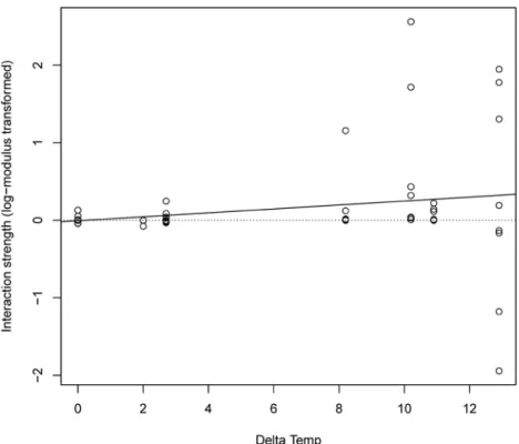
Figure A4: Ecological specialization of interaction strength in abiotic conditions. ... 14
16
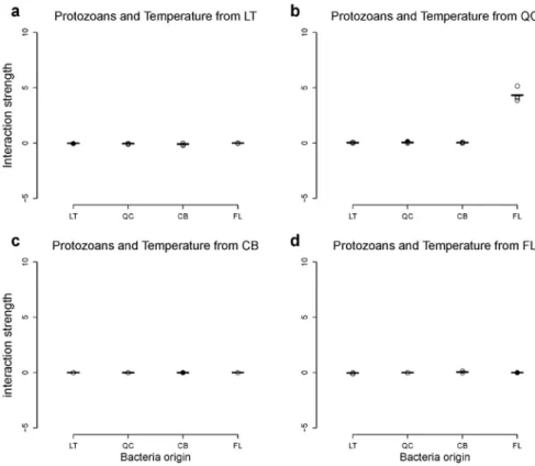
Figure A5: Response of interaction strength to biotic conditions for bacteria. ... 15
17
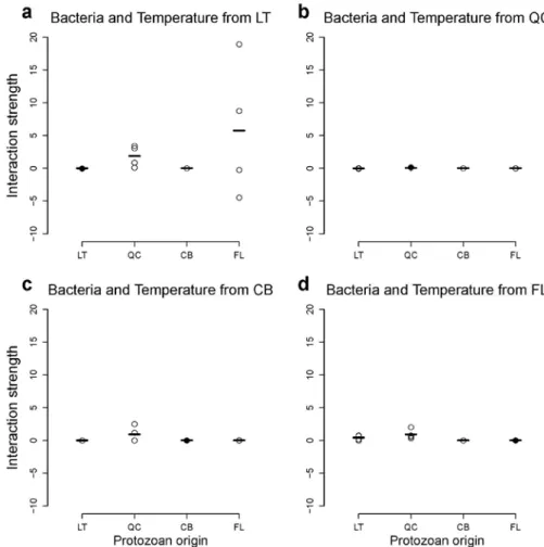
Figure A6: Response of interaction strength to biotic conditions for protozoans. ... 16
METHODS: Additional information on methodological procedures 19
Sample collection
20
The present study was conducted with inquiline communities that were collected from
21
Sarracenia leaves at two sites in the native range and two sites in the non-native range of the 22
plant’s distribution. Site selection was determined by the similarity in the average maximum
23
and minimum temperatures for July according to 30 years of data acquired by WorldClim
24
(www.worldclim.org). We therefore had duplicate native and non-native sites for the warm
25
and cold temperature limits of the plant species. The warm sites were Naczi Bog in Sumatra,
26
Florida (FL, native site, 30°16'32"N, 84°50'49"W, minimum and maximum July temperature:
27
21.6°C, 32.7°C) and Champ Buet in the low elevation of Switzerland (CB, non-native site,
28
46°36’50’’N, 6°34’50’’E, minimum and maximum July temperature: 18.9°C, 31.4°C). The
29
cold sites were Lac des Joncs in Saint-Fabien, Québec (QC, native site, 48°21'22"N,
30
68°49'29"W, minimum and maximum July temperature: 11.5°C, 22.4°C) and Les Tenasses in
31
the high elevation of Switzerland (LT, non-native site, 46°29’29’’N, 6°55’16’’E, minimum
32
and maximum July temperature: 9.2°C, 19.3°C) .
33
Teams in Switzerland, Québec and Florida simultaneously collected water from
34
mixed-aged leaves according to a shared protocol. Each member of the team was trained so
35
that little variation in the collection procedure would occur. At each field site, leaves were
36
randomly selected throughout the site. A sterilized pipette was used to gently mix the aquatic
37
community inside each leaf and deposit it into an autoclaved bottle. The process was
38
continued until 1L of pooled water from all randomly selected leaves was collected. In the
39
native sites, the top predator mosquito larvae were removed from the water immediately after
40
collection. Each of the 4 samples was then distributed in autoclaved bottles with enough
41 42
Switzerland was transported overnight to the Université du Québec à Rimouski (UQAR),
44
where the experiment took place. Samples that were collected in Québec remained at 4°C in
45
the laboratory during this time. All permits for collecting and shipping samples were acquired
46
before the start of the experiment.
47 48
Experimental design
49
Four incubators were set to reproduce the minimum and maximum daily July
50
temperatures for each of the four sites (Florida: 21.6°C, 32.7°C ; CB: 18.9°C, 31.4°C ; QC:
51
11.5°C, 22.4°C ; LT: 9.2°C, 19.3°C). Temperature linearly increased from 04h00 to 16h00
52
and decreased over the remainder of the 24 hour period. The incubators were also set to
53
follow a light:dark cycle of 12 hours, starting at 06h00. Temperature and light conditions
54
inside incubators were checked regularly, allowing us to assume that the experimental error
55
among incubators was negligible compared to the error due to the variability in the response
56
of bacteria and protozoans to the treatments. Inside incubators, tubes were placed in a random
57
block design, with the blocks rotated daily. The experiment lasted for 5 days, or an estimated
58
15 to 20 generations of protozoans (Lüftenegger et al. 1985) and 40 generations of bacteria
59 (Gray et al. 2006). 60 61 Experimental set-up 62
To start with a similar biomass of morphospecies in all replicates, initial population
63
sizes were 500 individuals for each flagellate, and 10 individuals for each ciliate. We used a
64
flow cytometer to measure the bacterial density in the bacteria cultures before the start of the
65
experiment. We then diluted the cultures of the four sites to a standardized concentration of
66
50'000 individuals of bacteria per mL. We then aliquoted 10 mL of this water into 50 mL
67
macrocentrifuge tubes in which the experiment took place. In each tube, 0.1 mL of water
containing the protozoan communities were introduced according to treatment. Note that
69
some contamination by local bacteria was unavoidable at this stage, but was assumed to be
70
negligible due to volume and density differences. A solution of 1 mL of autoclaved Tetramin
71
fish food (concentration of 6 mg of solid fish food in 1 mL of DI water, terHorst (2010)) was
72
added in all the tubes as the basal nutrient input for the communities.
73 74
Monitoring
75
We measured protozoan and bacterial density at the start of the experiment and after
76
five days of incubation. After gentle mixing of the community, an aliquot of 100 µL (1% of
77
the total volume; see Palamara et al. (2014)) from each sample was used to count the density
78
of protozoans with a Thoma cell microscope plate. If densities were too low for an accurate
79
Thoma cell microscope plate count, we used an entire microscope slide to count the density of
80
the protozoan in 100 µL. The density of bacteria was measured using a flow cytometer and
81
100 µL of each sample (Hoekman 2010).
82 83
Statistical analyses: one-tailed tests
84
For mixed-effects models using Temp or ∆Temp as explanatory variables, reported
p-85
values are one-tailed in accordance with the expected sign of the relationship. We chose the
86
best model based on BIC. In practice, when the sign of the relationship was not in the
87
expected direction, we computed the BIC for a model with the intercept only (no explanatory
88
variable), which corresponds to the best model in this situation. It is then necessary to correct
89
its BIC value by addition of the natural logarithm of the number of observations.
90 91 92
Statistical analyses: dealing with variability in interaction strength
94
Interaction strength was quantified using the index described by (Wootton 1997) and
95
Laska and Wootton (1998) with the index calculated as follows:
96
𝛾𝛾 = ln �𝐸𝐸𝐶𝐶� .𝑀𝑀 ,1
with E the abundance of the bacteria in the presence of protozoans, C the abundance of
97
bacteria in the absence of protozoans, and M the abundance of the protozoans.
98
This index is a compound of several measurements (E, C and M), and each has an associated
99
variance. In our case, we have four repetitions of each control density (for each origin), and
100
used their geometric average as C in the above equation. Furthermore, the division by M
101
strongly influences the variance of γ, with low values of M generating high variability. In
102
order to try to include this variability in our model we used the varIdent command, and
103
combining it with a varFix variance component assuming it was proportional to (var(Ci)/M)0.5, 104
with Ci as the four replicates of control density. However, this method was not sufficient to 105
circumvent the high variation issue, therefore we used Spearman correlation tests to analyze
106
our data.
107 108
Impact of abiotic and biotic conditions on protozoan species composition 109
We investigated the impact of the abiotic and biotic conditions on the community composition
110
at the end of the experiment with Canonical Correspondence Analysis (CCA). Note that the
111
composition was standardized for all tubes at the start of the experiment. We used the
log-112
transformed densities of the four protozoan morphospecies as response variable, and the
113
binary variables Local/Away for the biotic and the abiotic conditions as explanatory variables.
114
We added protozoan origin as a factor to account for intrinsic site differences. We performed
115
a CCA for each variable to obtain its overall contribution to the total variance of the data, and
116
partial CCA to estimate their exclusive contribution by controlling for both other variables.
Analyses were performed with the function cca of the vegan package (Oksanen et al. 2015) in
118
R (R Core Team 2015); the statistical significance of each variable considered globally was
119
evaluated with a permutation test with 10'000 simulations (function anova .cca of the vegan
120
package). The results are given in Table A5.
REFERENCES 122
Gray, S. M., T. E. Miller, N. Mouquet, and T. Daufresne. 2006. Nutrient limitation in
detritus-123
based microcosms in Sarracenia purpurea. Hydrobiologia 573:173-181.
124
Hoekman, D. 2010. Turning up the heat: temperature influences the relative importance of
125
top-down and bottom-up effects. Ecology 91:2819-2825.
126
Laska, M. S., and J. T. Wootton. 1998. Theoretical concepts and empirical approaches to
127
measuring interaction strength. Ecology 79:461-476.
128
Lüftenegger, G., W. Foissner, and H. Adam. 1985. r-and K-selection in soil ciliates: a field
129
and experimental approach. Oecologia 66:574-579.
130
Oksanen, J., F. G. Blanchet, R. Kindt, P. Legendre, P. R. Minchin, R. O'Hara, G. L. Simpson,
131
P. Solymos, M. H. H. Stevens, and H. Wagner. 2015. Package ‘vegan’. Community
132
ecology package, version:2.2-1.
133
Palamara, G. M., D. Z. Childs, C. F. Clements, O. L. Petchey, M. Plebani, and M. J. Smith.
134
2014. Inferring the temperature dependence of population parameters: the effects of
135
experimental design and inference algorithm. Ecology and Evolution 4:4736-4750.
136
R Core Team. 2015. R: A language and environment for statistical computing. R Foundation
137
for Statistical Computing, Vienna, Austria.
138
terHorst, Casey P. 2010. Evolution in response to direct and indirect ecological effects in
139
pitcher plant inquiline communities. The American Naturalist 176:675-685.
140
Wootton, J. T. 1997. Estimates and Tests of Per Capita Interaction Strength: Diet, Abundance,
141
and Impact of Intertidally Foraging Birds. Ecological Monographs 67:45-64.
142 143
Table A1 : Specialization to abiotic conditions for bacteria grown alone. Parameter estimates from 144
linear mixed effect models comparing distance to local temperature (∆Temp) and temperature effects on 145
bacteria when grown in the absence of protozoans. 146
147
Table A2 : Specialization to abiotic conditions for bacteria and protozoans. Parameter estimates from 148
linear mixed effect models comparing distance to local temperature (∆Temp) and temperature effects on 149
bacteria and protozoan densities from a subset of data where protozoan and bacteria origins matched, 150
and the bacteria and protozoan are grown together. 151
152
Random
effects Model Fixed effects Estimates SE DF t-value p-value BIC
Bacteria Bacteria origin ∆Temp Intercept 13.54 0.35 59 38.64 <0.001 154.7
∆Temp -0.03 0.02 59 -1.91 0.0030
Temperature Intercept 12.04 0.64 59 18.86 <0.001 126.5 Temperature 0.06 0.03 59 2.41 0.009
Random effects Model Fixed effects Estimates SE DF t-value p-value BIC
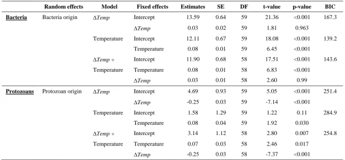
Bacteria Bacteria origin ∆Temp Intercept 13.59 0.64 59 21.36 <0.001 167.3
∆Temp 0.03 0.02 59 1.81 0.963 Temperature Intercept 12.11 0.67 59 18.08 <0.001 139.2 Temperature 0.08 0.01 59 6.45 <0.001 ∆Temp + Intercept 11.90 0.68 58 17.51 <0.001 143.6 Temperature Temperature 0.08 0.01 58 6.83 <0.001 ∆Temp 0.03 0.01 58 2.60 0.99
Protozoans Protozoan origin ∆Temp Intercept 4.69 0.93 59 5.05 <0.001 251.4
∆Temp -0.25 0.03 59 -7.14 <0.001 Temperature Intercept 1.58 1.29 59 1.22 0.11 284.9 Temperature 0.08 0.04 59 1.92 0.030 ∆Temp + Intercept 3.14 1.12 58 2.80 0.007 254.8 Temperature Temperature 0.07 0.03 58 2.46 0.017 ∆Temp -0.25 0.03 58 -7.37 <0.001
Table A3 : Specialization to biotic conditions for bacteria and protozoans. Parameter estimates from 153
linear mixed effect models comparing specialization of bacteria and protozoans to biotic conditions. 154
Using two subsets of data, one where bacteria grew in their own temperature with the different 155
protozoan origins and the second one where protozoans grew in their own temperature with the different 156
bacteria origins. "Local" indicates the conditions where bacteria, protozoans and temperature were from 157
the same origins. "Away" indicates the cases where the origins of the two trophic levels did not match. 158
159 160 161
Table A4: Relative importance of specialization to biotic and abiotic conditions for protozoans. 162
Parameter estimates from linear mixed effect models comparing specialization of bacteria and 163
protozoans to biotic and abiotic conditions both expressed as "Local/Away" binary variables. 164
165 166
Random effects Model Fixed effects Estimates SE DF t-value p-value
Bacteria Bacteria origin Local vs. Away Intercept (Away) 13.65 0.30 59 45.07 <0.001
Local 0.03 0.33 59 0.09 0.465
Protozoans Protozoan origin Local vs. Away Intercept (Away) 3.90 0.90 59 4.34 <0.001
Local 0.88 0.45 59 1.97 0.027
Random effects Model Fixed effects Estimates SE DF t-value p-value
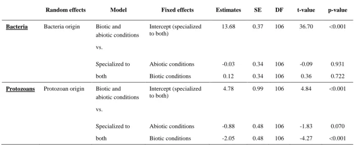
Bacteria Bacteria origin Biotic and
abiotic conditions
Intercept (specialized to both)
13.68 0.37 106 36.70 <0.001
vs.
Specialized to Abiotic conditions -0.03 0.34 106 -0.09 0.931 both Biotic conditions 0.12 0.34 106 0.36 0.722
Protozoans Protozoan origin Biotic and
abiotic conditions
Intercept (specialized to both)
4.78 0.99 106 4.84 <0.001
vs.
Specialized to Abiotic conditions -0.88 0.48 106 -1.83 0.070 both Biotic conditions -2.05 0.48 106 -4.27 <0.001
Table A5 : Results of Canonical Correspondence Analysis (CCA). The overall and exclusive (i.e., 167
controlling for the other variables using partial CCA) contributions of the three explanatory variables 168
are given, with the corresponding statistics and p-values. Percentage contributions are in parenthesis. 169
170
Inertia Permutation test
Explanatory variable Global Exclusive Chi2 F p-value
Protozoan origin 0.362 (25.1%) 0.373 (25.9 %) 0.362 17.10 <0.001
Local/Away for biotic conditions 0.015 (1.0 %) 0.020 (1.4 %) 0.015 1.59 0.066
Local/Away for abiotic conditions 0.010 (0.7%) 0.021 (1.5%) 0.010 1.09 0.160
171 172
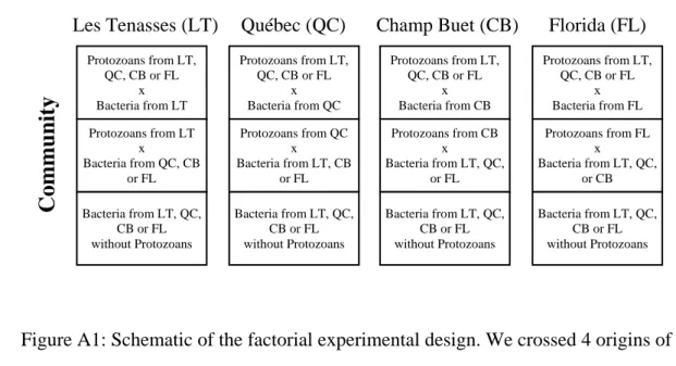
Figure A1: Schematic of the factorial experimental design. We crossed 4 origins of protozoan
173
communities with 4 origins of bacteria communities (Les Tenassses (LT), Québec (QC),
174
Champ Buet (CB), and Florida (FL) in both cases), and grew each combination in 4
175
incubators set to the average temperatures of month of July for the 4 sites (LT = 14.2°C,
176
QC = 17°C, CB = 25.2°C, and FL = 27.2°C ). The temperatures varied through time over a
177
cycle of 24 hours (see details in the Methods section).
178 Protozoans from LT, QC, CB or FL x Bacteria from LT Protozoans from LT x Bacteria from QC, CB or FL Bacteria from LT, QC, CB or FL without Protozoans Protozoans from LT, QC, CB or FL x Bacteria from QC Protozoans from QC x Bacteria from LT, CB or FL Bacteria from LT, QC, CB or FL without Protozoans Protozoans from LT, QC, CB or FL x Bacteria from CB Protozoans from CB x Bacteria from LT, QC, or FL Bacteria from LT, QC, CB or FL without Protozoans Protozoans from LT, QC, CB or FL x Bacteria from FL Protozoans from FL x Bacteria from LT, QC, or CB Bacteria from LT, QC, CB or FL without Protozoans
Les Tenasses (LT) Québec (QC) Champ Buet (CB) Florida (FL)
Co
m
m
uni
ty
Temperature
179
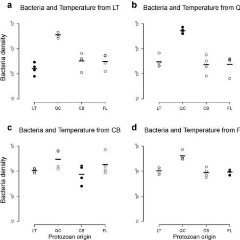
Figure A2: Response of bacteria to biotic conditions. This figure shows the response of
(log-180
transformed) densities (individuals/mL) of bacteria when grown in their local temperature, in
181
the presence of protozoans from the different origins. The black dots indicate the cases where
182
bacteria were grown in their local temperature with the protozoans from their origin. This
183
figure does not show any evidence of specialization to biotic conditions for bacteria. Legend
184
as in Fig. A1.
186
Figure A3: Response of interaction strength to abiotic conditions. This figure shows the
187
response of interaction strength between bacteria and protozoans from the same origins when
188
grown together in the different temperatures. The black dots indicate cases where bacteria and
189
protozoan from the same origin were in their local temperature. This figure illustrates the high
190
variation between each treatment. Note that the estimated values of interaction strength were
191
positive in several cases, indicating that density of bacteria was higher in the presence of
192
protozoans than without. Although we cannot exclude measurement errors, a potential
193
explanation is preferential feeding of protozoan for large bacteria, allowing smaller species to
194
become more abundant. This may lead to a switch towards communities dominated by small
195
species which could have a higher density but a lower biomass than communities with more
196
large bacteria species. Legend as in Fig. A1.
198
Figure A4: Ecological specialization of interaction strength in abiotic conditions. Using the
199
same data as in Fig. S3, interaction strength (log-modulus transformed) is expressed as a
200
function of ∆Temp (Delta Temp). Using Spearman rank correlation, we found that interaction
201
strength was positively related to ΔTemp, with ρ = 0.298, p-value = 0.014 (p-value from
202
permutation test with 10'000 simulations). The effect of protozoans on bacteria became
203
weaker when moving away from the local temperature, consistent with protozoans being at an
204
optimum in their local abiotic condition. The fitted line is from a linear regression.
206
Figure A5: Response of interaction strength to biotic conditions for bacteria. This figure
207
shows the response of interaction strength when bacteria grew in their local temperature, but
208
in the presence of protozoans from the four origins. The black dots indicate the cases where
209
bacteria, protozoan and temperature origins matched. This figure does not show any evidence
210
of specialization of bacteria to biotic conditions. Legend as in Fig. A1.
212
Figure A6: Response of interaction strength to biotic conditions for protozoans. This figure
213
shows the response of interaction strength when protozoans grew in their local temperature,
214
but in the presence of bacteria from the four origins. The black dots indicate the cases where
215
bacteria, protozoans and temperature origins matched. This figure does not show any
216
evidence of specialization of protozoans to biotic conditions. Legend as in Fig. A1.