HAL Id: hal-01448127
https://hal.uca.fr/hal-01448127
Submitted on 27 Jan 2017
HAL is a multi-disciplinary open access
archive for the deposit and dissemination of
sci-entific research documents, whether they are
pub-lished or not. The documents may come from
teaching and research institutions in France or
abroad, or from public or private research centers.
L’archive ouverte pluridisciplinaire HAL, est
destinée au dépôt et à la diffusion de documents
scientifiques de niveau recherche, publiés ou non,
émanant des établissements d’enseignement et de
recherche français ou étrangers, des laboratoires
publics ou privés.
Changing the routing protocol without transient loops
Nancy Rachkidy, Alexandre Guitton
To cite this version:
Nancy Rachkidy, Alexandre Guitton. Changing the routing protocol without transient loops.
Com-puter Communications, Elsevier, 2016, 82, pp.49 - 58. �10.1016/j.comcom.2016.02.010�. �hal-01448127�
Changing the Routing Protocol without Transient Loops
Nancy El Rachkidy, Alexandre Guitton∗
Clermont Universit´e, Universit´e Blaise Pascal, LIMOS, BP 10448, F-63000 Clermont-Ferrand, France CNRS, UMR 6158, LIMOS, F-63173 Aubi`ere, France
Abstract
Computer networks generally operate using a single routing protocol. However, there are situations where the routing protocol has to be changed (e.g., because an update of the routing protocol is available, or because an external event has triggered a traffic with different quality of service requirements). In this paper, we show that an uncontrolled change of the routing protocol might yield to transient routing loops (even if the involved routing protocols are loop-free). We show that it is possible to achieve a loop-free change for multiple destinations using a strongly connected component approach producing successive steps, where each step contains nodes that can change the routing protocol in parallel. Our aim is to reduce the number of steps in order to reduce the time required for the network to change from one routing protocol to another. Simulation results show that our strongly connected component approach greatly reduces the number of steps compared to the state of the art, and thus it greatly reduces the time for the change. Keywords: Routing protocols, routing protocol change, transient routing loops.
1. Introduction
Computer networks generally operate a single routing protocol which determines the route packets have to follow in order to reach a destination. However, some situations require to change the current routing protocol. For example, this change might be triggered by the availability of a major update of the protocol or the correction of a security issue [1]. Another example concerns monitoring applications in wireless sensor networks, where the detection of a critical event might trigger the change from an energy-efficient routing protocol to a delay-sensitive routing protocol [2]. Another example focuses on the changes in routing decisions caused by major modifications of the topology (due to link or node failures, or to significant changes in routing metrics) [3, 4, 5].
If nodes are accurately synchronized, they can perform the change simultaneously from the current
routing protocol R1to the new routing protocol R2. However, this solution is often difficult to implement in
practice, especially in large networks. Indeed, the cost of an accurate synchronization might be prohibitive, or nodes might be operated by different network administrators, leading to different plannings for the change. We assume in the following that nodes cannot be synchronized in such a precise manner.
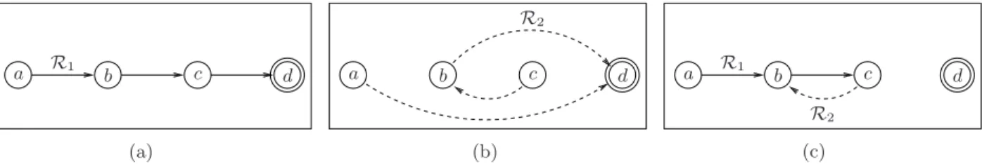
If nodes are not synchronized and if nodes perform the change arbitrarily, transient routing loops might occur, even if the routing protocols are loop-free when considered independently. Figure 1 shows such an
example. Initially, all packets towards d are routed according to routing protocol R1, and R1 is loop-free
(see Figure 1(a)). If nodes are requested to change to another protocol R2 in arbitrary order (R2is shown
on Figure 1(b)), it is possible that c changes first, resulting into the routing depicted on Figure 1(c). In this case, a transient routing loop occurs between nodes b and c. This loop will eventually disappear when node
b changes to R2too, but the impact on the network performance is not negligible.
∗Corresponding author.
Email Address: [email protected](Alexandre Guitton) Phone: +33 473405229, Fax: +33 473407639
a a a R1 b c d b c d R1 b c d R2 R2 (a) (b) (c)
Figure 1: Uncontrolled changes might yield to routing loops. (a) The initial routing protocol R1 is loop-free for destination d.
(b) The new routing protocol R2 is also loop-free for destination d. (c) A loop occurs between nodes b and c, if a and b route
according to R1and c routes according to R2.
Routing loops reduce network performance as they can cause node inaccessibility issues or overload the network. Even if the routing loops caused by the changes are transient (because all nodes will eventually perform the change to the new, loop-free routing protocol), our aim is to completely avoid them, as they might have a significant impact for the applications.
In [6], we classified routing protocols into three categories: (i) compatible routing protocols, which do not yield to routing loops when they are used together, (ii) delayable routing protocols, where nodes might avoid loops based on the knowledge of the distance functions of the two protocols, and (iii) combined routing protocols, when the distance functions of the two protocols are not known or hard to compute locally by the nodes. In [7], we use a probabilistic approach to avoid loops. Indeed, some nodes choose randomly whether to forward packets or to hold them. However, the common assumption of [6, 7] is that routing protocols alternate. In this paper, we make a more general assumption, where the change is final: once a node has
changed to R2, it does not change back to R1 anymore. This new assumption makes the previous solutions
inapplicable. Moreover, we show that the change to R2can be performed in successive steps, where all nodes
of the same step can perform the change arbitrarily without causing loops.
Our contribution is three-fold. First, we show that the probability of transient loops is high for both random and real topologies, and for several types of routing protocols pairs. Second, we improve the main heuristic proposed by [8] for networks with several destinations, by proposing a greedy mechanism to deal with troublesome destinations, and by computing a sequence of steps rather than a sequence of nodes. Third, we propose our centralized heuristic based on the computation of strongly connected components in order to classify nodes into steps. It is aimed at reducing the overall number of steps and thus reducing the change duration, which is our main metric.
The remainder of the paper is organized as follows. Section 2 describes relevant research works of the literature. Section 3 first presents two improvements for the main protocol of the literature [8]: a greedy mechanism for the per-destination ordering, and the computation of a sequence of steps rather than a sequence of nodes. Then, it presents our central theorem based on strongly connected components. Finally, it presents our heuristic based on this theorem. Section 4 evaluates the performance of these heuristics on several topologies and for several routing protocols pairs. Finally, Section 5 concludes this work.
2. Related work
In this section, we first describe architectures where routing loops might occur. Then, we present the solutions from the literature that avoid routing loops occurring during the change from one protocol to another. Then, we describe in details the Routing Tree Heuristic (RTH) presented in [8], as it is the main heuristic to change routing protocols. Finally, we describe the main differences between RTH [8] and this paper.
2.1. Networks and protocols with risks of loop occurrence
Several routing protocols that combine different routing decisions have been proposed in the literature. In [9], the authors propose to combine a reactive routing protocol with a greedy geographical routing protocol. When a packet has to be forwarded, the reactive protocol establishes the whole route to the destination. The
geographical protocol is used when the next-hop according to the reactive protocol becomes unreachable. Routing loops can occur if the geographical protocol forwards packets to a node that uses the reactive
protocol. In [10], a routing protocol Rd that reduces delay is combined with a routing protocol Re that
reduces energy. Rd and Re are used depending on the traffic produced by the application: urgent packets
are forwarded according to Rd, while periodic packets are forwarded according to Re. Routing loops can
occur if an urgent packet reaches a node that has a limited energy and uses Re. In [11], packets are given
a priority based on traffic type. The next-hop of a packet is computed according to several parameters, including packet priority, number of hops to the destination, link quality for the next-hop, residual energy for the next-hop, load of the next-hop, etc. Routing loops can occur if the parameters used by a node are different from the parameters used by another node on the path to the destination.
Multi-purpose Wireless Sensor Networks (WSNs) [12] have been proposed to enable a single WSN de-ployment to support several applications. The main advantage of multi-purpose WSNs is that the cost of deployment is shared by all the applications. Several researchers have proposed protocols for multi-purpose WSNs [13, 14, 15, 16]. In such networks, several routing protocols can be used simultaneously, because the large amount of applications yield to different requirements that cannot be met by a single routing protocol. However, dealing with several routing protocols might cause routing loops when the choice of the routing protocol is made locally by each node [6, 7].
2.2. Heuristics that avoid routing loops
The problem of avoiding transient loops during a change of routing protocols is a recent issue. We summarize here the main related works.
In [6, 7], nodes are synchronized and forward packets according to a schedule composed of two periods p1
and p2. During p1, nodes forward packets according to R1, and during p2, nodes forward packets according
to R2. Routing loops can occur if nodes become desynchronized or if the decision to forward a packet
according to R1 or R2 is made locally by each node, independently of the period. In [6], properties of
pairs of routing protocols are studied, and three categories are identified: (i) compatible routing protocols, which do not yield to routing loops, (ii) delayable routing protocols, where nodes might avoid loops based on the knowledge of the distance functions of the two protocols, and (iii) combined routing protocols, where the distance functions of the two protocols are not known or hard to compute locally by the nodes. The
last two categories require R1 and R2 to alternate, as some nodes hold packets indefinitely for one routing
protocol. They are not suitable for a final change of routing protocol, as we consider in this paper. In [7], two heuristics are proposed to avoid loops or reduce their occurrences. In the first heuristic, all loops are avoided
by forbidding some nodes to forward packets according to one routing protocol Ri. In the second heuristic,
a probabilistic approach is used to reduce the risk of loops: nodes that could potentially be involved in loops choose randomly whether to forward or to hold packets for one routing protocol. These two heuristics cannot
be applied here because the change from R1to R2 is final: once a node has performed the change to R2, it
does not change back to R1.
In [4], the authors show that most routing protocols can produce transient routing loops after a topological change. They show that such loops can be avoided by having routers process routing updates in a specific order. Their mechanism is able to deal with link failures, new links, or updates on link metrics. The
differences with this paper are the following: (i) we consider arbitrary protocols for R1 and R2, while [4]
considers a single routing protocol on two similar topologies, (ii) we reduce the number of steps required for the change, while [4] provides an ordering of updates that does not cause loops, and (iii) in our proposition, each node is updated exactly once for each destination, while the algorithm of [4] might update the same node several times.
In [3, 5], the authors show that ordering the routing updates yields to additional message overhead and increases the change delay. They avoid transient routing loops by exploiting the existence of one forwarding table per interface. Messages arriving through unexpected interfaces are discarded, because they indicate a discrepancy between the view of the router and of its neighbors. Once all routers have the same view of the topology, the protocol converges and produces loop-free routes. The main difference with this paper is that we do not drop packets during the change to reduce the impact of loops, but we avoid changing the routing protocol of nodes if it causes a loop.
In [17, 18], the authors show that transient routing loops that occur after topological changes can be avoided by applying a sequence of topology updates. Between two topology updates, the same routing protocol is used, but some link values are modified, which result into changes in routing decisions. They propose a protocol that minimizes the number of topology updates. The difference with this paper are the following: (i) we consider two different routing protocols on a single topology, while [17, 18] consider a single routing protocol applied on a sequence of updated topologies, (ii) we consider arbitrary routing protocols, while [17] considers changes on only one link and [18] considers changes concerning the links of a single router, and (iii) we reduce the number of steps to perform the change, where each step is a set of nodes and each node appears exactly once per destination, while [17, 18] attempts to minimize the number of topology updates to guarantee the convergence of a single routing protocol without transient loops.
In [8], the authors describe a heuristic which is based on similar assumptions as in this paper. We describe this heuristic in details in the next subsection.
2.3. Routing Tree Heuristic [8]
In [8], authors proposed ordering algorithms in order to avoid loops during the change from one routing
protocol R1to another routing protocol R2. They proposed a heuristic called Routing Tree Heuristic (RTH).
RTH consists of the following. For each destination d, the ordering constraints are computed separately.
First, a greedy algorithm is used to compute the set Sdof nodes that do not yield to loops in the network. A
node is added to Sdif and only if its next-hops using R1 and using R2 are already in Sd. Second, the set ¯Vd
of nodes is built by adding each node that does not have the same next-hops using R1and R2. Third, RTH
builds a set of constraints C in the following way: for each path on R2from a source node to the destination
d, a constraint is generated for the last pair of nodes (u, v) on this path such that u ∈ ¯Vd and u /∈ Sd. In
this way, the change from R1to R2 starts from the destination backwards (according to R2) to the sources,
which guarantees that no loop occur on the path. This means that a node n does not change before all its
successors on R2 have already changed. Finally, RTH creates an acyclic directed graph GC from the set of
constraints C, and the ordering is computed as a topological sort of GC.
2.4. Differences between RTH and our proposition The differences with this paper are the following:
• RTH changes the routing protocol of nodes one by one, so the duration of the change is proportional to the number of nodes in the network. However, we show here that it is possible to change the routing protocol of several nodes in parallel, without any loop occurrence. We use this parallelism to reduce the time required for the routing protocol change.
• RTH changes the routing protocol of nodes by following the arcs of R2from the destination backwards
to the sources. However, we show that it is possible to change the routing protocol for nodes
indepen-dently of their position on the paths from sources to destinations according to R2. We use a strongly
connected component approach to identify those nodes.
• The authors of RTH assume that there are few troublesome destinations, so RTH tries to compute the ordering for all destinations together when possible. However, we show that troublesome destinations are relatively frequent, so we decided to consider destinations independently.
3. Fast changes of routing protocols
The main criteria when performing changes of routing protocols without transient loops is the overall time required for the change. We consider in this paper that it is possible to perform the change as a sequence of steps, where nodes of each steps can change their routing protocol in parallel. Thus, the time required for the change is proportional to the number of steps, rather than to the number of nodes in the network.
In this section, we first describe improvements to RTH [8]: the first improvement is a greedy mechanism that deals with troublesome destinations, and the second improvement enables the support of steps. Second, we give a mathematical background for parallel steps based on strongly connected components. Third, we describe our heuristic based on this background.
3.1. Improvements of RTH
We present here two improvements of RTH. The first improvement describes the per-destination ordering, when a per-router ordering does not exist due to troublesome destinations. The second improvement describes how to enable parallel changes in RTH.
3.1.1. Improvement 1: Greedy mechanism of per-destination ordering in RTH
The first improvement is a greedy mechanism of per-destination ordering. Note that this ordering can be applied when a per-router ordering exists (in this case, all destinations can be regrouped, and the re-sult is the same as with the original RTH) as well as when a per-router ordering does not exist (in this case, several destinations are regrouped in a greedy manner, and troublesome destinations are processed independently). Authors of [8] mainly described the per-router ordering (which assumes that there is no troublesome destination), and explained that troublesome destinations can be processed independently from the other destinations. However, they did not propose an algorithm that identifies troublesome destinations, or that aggregates non-troublesome destinations (this was left as future work due to the fact that troublesome destinations were limited in their experimental evaluation, cf Subsection V.C of [8]).
The RTH heuristic (see Figure 8 of [8]) is modified in the following way. Initially, the set of troublesome
destinations is initialized to ∅. In the main loop that considers each destination d, the constraint graph GCis
computed using V and the set of constraints C. If the new graph GC, including the constraints generated by
all previous non-troublesome destinations and the new destination d, has no loop, then the new destination
is considered as a non-troublesome destination. However, if the new graph GC has a loop, destination d
is added to the list of troublesome destinations, and the constraints generated from this destination are
removed from C. In this case, modifications to GC concerning d are discarded. After all destinations have
been considered, the ordering is made first for all non-troublesome destinations together using GC, and then
for all troublesome destinations one by one, using the per-destination ordering. 3.1.2. Improvement 2: Parallel changes in RTH
The second improvement consists of enabling parallel changes in RTH, in order to obtain a sequence of steps rather than a sequence of nodes. This modification can be performed efficiently from the constraint
graph GC computed for all non-troublesome destinations (as well as for each troublesome destination
inde-pendently). This improvement consists of changing the last step of RTH, by replacing the topological sort
of GC with Algorithm 1. In this algorithm, a new set S is added to sequence T at each iteration. At each
iteration, all nodes that have no incoming edges in GC (that is, no constraints), are added to the new set S
and all edges leaving from these nodes are removed from GC. Since GC has no loop (due to the construction
of all non-troublesome destinations, and to the fact that troublesome destinations are considered indepen-dently), the process ends with all nodes being in T . In our implementation, sequence T contains first the steps for all non-troublesome destinations, then the steps for each troublesome destination successively.
In the following, we denote by RTH-p this heuristic. 3.1.3. Example of RTH-p
In the following, we describe RTH-p in an example. This example shows our greedy mechanism for per-destination ordering, as well as parallel changes.
Figure 2 shows a graph of five nodes, with three destinations and two routing protocols: (a)
destina-tion a with Ra 1 and R a 2, (b) destination d with R d 1 and R d
2, and (c) destination e with R
e
1 and R
e
2. When
considering destinations independently, RTH produces the order (a, e, d, c, b) for destination a, (d, e, a, b, c) for destination d, and (e, d, c, b, a) for destination e. When considering all destinations together, our greedy mechanism first considers destination a, identifies destination d as troublesome, and identifies destination e as non-troublesome. Thus, RTH-p produces sequence ({d, e}, {c}, {b}, {a}) for both non-troublesome des-tinations a and e, and sequence ({a, d, e}, {b}, {c}) for troublesome destination d. The resulting sequence is ({d, e}, {c}, {b}, {a}, {a, d, e}, {b}, {c}) (to simplify the notation, we did not indicate which destination is concerned by the change at each step). Note that each node appears several times but for different destinations.
Algorithm 1Parallel changes in RTH.
Require: GC a graph of constraints
Ensure: T is a sequence of steps
T ← ∅
whilesome nodes are not in T do
S ← ∅
whilenode n ∈ GC do
if n /∈ S and n /∈ T then
if n has no incoming edges in GC then
S ← S ∪ {n} end if
end if end while
whilenode n ∈ S do
remove from GC all edges leaving from n
end while
add set S to sequence T end while Ra1 R a 2 Rd1 Rd2 Re1 Re2 (a) (b) (c) a a a b c d b c d b c d e e e
Figure 2: Example of routing protocols for three destinations: (a) a is the destination, (b) d is the destination, and (c) e is the destination.
3.2. Problem formulation for the construction of sequence of steps
Let V be a set of nodes and d ∈ V a destination. Let us consider two routing protocols for destination d:
R1is the routing protocol initially used by nodes, and R2 is the new protocol to use. For all i ∈ {1, 2} and
for all n ∈ V , we denote by Ri(n) ∈ V the next-hop of n towards d according to Ri. Given a partition
(V1, V2) of V (i.e., V1∪ V2= V and V1∩ V2= ∅), we denote by RV1,V2 the routing protocol defined in the
following way: for all n ∈ V1, RV1,V2(n) = R1(n), and for all n ∈ V2, RV1,V2(n) = R2(n). In other words,
nodes of V1 route according to R1, and nodes of V2 route according to R2. The set of routing decisions of
both R1 and R2 form the set E of the edges of the graph G = (V, E).
Definition 1 (Loop-free step). Let (V1, V2) be a partition of nodes, and S ⊂ V1 a set of nodes that change
their routing protocol to R2 in arbitrary order. S is called step. Step S is said to be loop-free if and only if
for all S′ ⊂ S, the routing protocol RV1\S′,V2∪S′ is loop-free.
Definition 1 states that a step S is loop-free if and only if all the possible intermediate sub-steps S′⊂ S
correspond to a loop-free routing protocol. This means that the nodes of S can change their routing protocol arbitrarily without causing loops.
Definition 2 (Loop-free sequence). Let T = (S1, . . . , Sm) be a sequence of steps. Sequence T is said to be
loop-free if and only if both conditions apply:
• (S1, S2, . . . , Sm) partitions the set V ,
• for all i ∈ [1; m], Siis a loop-free step on partition (V1i, V
i 2), with V i 2 = S1∪ . . . ∪ Si−1 and V1i= V \V i 2.
Definition 2 states that a sequence T = (S1, . . . , Sm) is loop-free if and only if each step Si is loop-free,
and after step Sm, all nodes belong to V2m∪ Sm = V (that is, they have changed to the target routing
protocol R2). Note that the set of nodes running R2, which is V2i, increases as the sequence progresses.
Figure 3 shows an example of loop-free sequence T = ({a, b, d}, {c}). Figure 3(a) shows the initial
routing protocol R1. Figure 3(b) shows both R1 and R2for nodes of the first step {a, b, d}, to indicate that
these nodes might route either according to R1 (if they have not changed yet) or R2 (if they have already
changed). It can be seen that for any routing protocol used by the nodes of the first step, no loop occurs
for any arbitrary order of change. Figure 3(c) shows R2 for nodes that have changed their routing protocol
on the previous step, and shows both R1and R2 for the node of the second step. On a side note, it can be
noticed that T is a loop-free sequence with a minimum number of steps, as it is not possible to have both b and c in the same loop-free step.
a a a b c d b c d b c d R1 R1 R1 R2 R2 (a) (b) (c)
Figure 3: An example of loop-free sequence T = ({a, b, d}, {c}). (a) Initially, all nodes route according to R1. (b) During the
first step, nodes from {a, b, d} might route according to R1 or R2 without causing loops. (c) During the second step, node c
routes according to R1 or R2, while all nodes from {a, b, d} route according to R2. At the end of the second step, all nodes
route according to R2(not shown).
Theorem 1. Let G, V1, V2, R1 and R2 be defined as previously for a destination d. Let G′= (V, E′) with
E′ ⊂ E, such that for all x ∈ V
1, (x, R1(x)) ∈ E′ and (x, R2(x)) ∈ E′, and for all x ∈ V2, (x, R2(x)) ∈ E′.
Let C = {Ci}i be the set of all strongly connected components of G′. For all i, let us denote by Ci′⊂ Ci a set
of nodes that verifies the following properties:
• C′
• G′
i= (V, Ei′) does not contain any loop, with Ei′ defined as follows:
– if x ∈ C′
i then (x, R1(x)) ∈ Ei′ and (x, R2(x)) ∈ Ei′,
– if x ∈ V1\Ci′ then (x, R1(x)) ∈ E′i,
– if x ∈ V2 then (x, R2(x)) ∈ Ei′.
Then, S = ∪iCi′ is a valid step for destination d.
Proof. Let us assume that {C′
i}i verifies the properties. We have to show that S = ∪iCi′ is a valid step, that
is, for every S′⊂ S, R
V1\S′,V2∪S′ is loop-free and leads to destination d. Let S′ be an arbitrary subset of S,
and let us build RV1\S′,V2∪S′.
Let us first show that RV1\S′,V2∪S′ is loop-free. By contradiction, let us suppose that there is a loop
(x0, x1, . . . , xn) in RV1\S′,V2∪S′, with xn = x0.
• Suppose here that this loop spans a single strongly connected component Ci. For all k, we have
(xk, xk+1) ∈ ES′. (i) If xk ∈ S′, then xk+1 = R2(xk) by construction of ES′ (since S′ ⊂ S ⊂ Ci′).
Because of the properties of C′
i, we have (xk, R2(xk)) ∈ Ei′. (ii) If xk ∈ S/ ′ and xk ∈ V1, then
xk+1= R1(xk) by construction of ES′. We have to consider the two following sub-cases: xk∈ Ci′ and
xk ∈ C/ i′. If xk ∈ Ci′, then (xk, R1(xk)) ∈ Ei′. If xk ∈ C/ i′, then (xk, R1(xk)) ∈ Ei′. (iii) If xk ∈ S/ ′
and xk ∈ V2, then xk+1= R2(xk) by construction of ES′, and xk ∈ C/ i′. Thus, (xk, R2(xk)) ∈ Ei′. To
summarize these three cases, all the arcs of the loop on ES′ are also included in the arcs of Ei′, thus
G′
i contains a loop. However, this is impossible by construction of Ci′. Thus, by contradiction, there is
no loop on GS′.
• Suppose now that this loop spans several strongly connected components, including Ci and Cj, with
i 6= j. For all nodes xm of the loop (with (xm, xm+1) ∈ ES′), let us show that (xm, xm+1) ∈ E′. (i) If
xm∈ S′, then xm+1= R2(xm), and xm∈ Ci′, which means that xm∈ V1. Thus, (xm, R2(xm)) ∈ E′by
construction of E′. (ii) If x
m∈ S/ ′ and xm∈ V1, then xm+1= R1(xm). Thus, (xm, xm+1) ∈ E′. (iii) If
xm∈ S/ ′and xm∈ V2, then xm+1= R2(xm). Thus, (xm, xm+1) ∈ E′. To summarize these three cases,
for all xmof the loop, (xm, xm+1) ∈ E′, so there exists a loop in G′ between a node of Ci and a node
of Cj, which means that Ci and Cj are the same strongly connected component, which is impossible.
Let us show now that for any node x, d is reachable from x in GS′. By contradiction, let us suppose that
there is a node x from which d is not reachable. Let us consider the path starting from x in GS′. Either
there exists a node on the path that has no next-hop on GS′, or the path has a loop. We just proved that
there is no loop in GS′, so there has to be a node y without a next-hop. By construction of GS′, we can see
that all nodes y ∈ S′∪ (V
1\S′) ∪ V2= V have a next-hop, so destination d is reachable from any node x in
GS′. This completes the proof.
Figure 4 shows an example of a graph of nine nodes, where destination is node f . The routing protocols R1
and R2 are shown on Figure 4(a). To build the first valid step, all routing arcs are considered. The strongly
connected components of the resulting graph are the following: C1= {f }, C2= {b, c} and C3= {a, d, e, g, h, i}.
The following sets verify the property of the theorem: C′
1= {f }, C′2 = {b} and C′3 = {d, g, h, i}. Indeed,
it can be verified that none of the graphs G′
i (for i ∈ {1, 2, 3}) has a loop (this can also be seen on the
graph shown on Figure 4(b)). Thus, the step S1= {b, d, f, g, h, i} is a valid first step. To build the second
valid step, the strongly connected components of the graph shown on Figure 4(c) are computed. They are
the following: C1 = {a}, C2 = {b}, . . . , C9 = {i}. The following sets verify the property of the theorem:
C′ 1= {a}, C ′ 3 = {c}, C ′ 5= {e}, and C ′
i = ∅ otherwise. The second step is S2= {a, c, e}. After this step, all
nodes route according to R2. Thus, T = (S1, S2) is a loop-free sequence.
3.3. Centralized heuristic for loop-free change of routing protocols
In this subsection, we describe our centralized heuristic for loop-free change, called Strongly Connected component Heuristic with parallel changes (SCH-p). We assume that a centralized entity knows the whole
a a a b c b c b c d d d e f e f e f g g g h i h i h i (a) (b) (c)
Figure 4: Sequence based on strongly connected components. (a) The graph has three strongly connected components C1= {f },
C2= {b, c}, C3= {a, d, e, g, h, i}. (b) The first step is S1= {b, d, f, g, h, i}, and only the nodes of S1can route according to R1
or R2. (c) The second step is S2= {a, c, e}, and only the nodes of S2 can route according to R1or R2.
SCH-p is based on Algorithm 2. Each destination is considered sequentially and independently. First, the set of strongly connected components of the graph is built based on the two routing protocols for the
current destination. Then, each strongly connected component Ci is considered individually, and nodes are
distributed into several steps according to Algorithm 3. We use a greedy approach: for each step Sj, we add
nodes one by one into a set C′
i,j, until it is not possible to add more nodes without violating the constraints
of Theorem 1. Then, we move to the next step, until all nodes of Ci are in a step for this destination.
The worst-case complexity of SCH-p is O(|V |5). Indeed, there are at most |V | destinations. For each
destination, the strongly connected components of a graph can be computed in O(|V | + |E|) with Tarjan’s algorithm [19]. Note that in our graphs, |E| ≤ 2|V | as each node has at most two outgoing arcs (one with
R1and one with R2). For each strongly connected component Ci, there are at most |Ci| resulting steps (as
there is at least one node per step). Computing the set C′
i,j requires considering at most |Ci|2 combinations
of nodes, each requiring to build G′ and determining if it has a loop, which can be done in O(|C
i|). As the
set of strongly connected components partitions the graph, we obtain the overall complexity of O(|V |5).
4. Simulation results
In this section, we describe our simulation results. We start by describing our settings. Then, we quantify the probability of loop occurrence when using arbitrary routing protocols, with uncontrolled changes (that is, without any heuristic to avoid transient loops). We also quantify the number of troublesome destinations for RTH and RTH-p. Then, we compute the number of steps required to change the routing protocols for RTH, RTH-p and our heuristic SCH-p.
4.1. Topologies and parameter settings
We used two types of topologies in order to evaluate the heuristics over a large number of networks. First, we decided to generate random connected graphs. We generated networks composed of 50, 100, 150, 200, 250, and 300 nodes, randomly deployed on an area of 100m×100m. Nodes that are distant of less than 20 m are considered connected. Second, we decided to test our heuristic SCH-p on real networks. We used the Rocketfuel network topologies [20, 21], which are also used for the evaluation of RTH in [8]. The resulting topologies have 79, 87, 104, 138, 161, and 315 nodes.
In the following, we use three scenarios for the routing protocols. They are all based on shortest paths,
using different link metrics. In Scenario 1, R1 uses the hop-count metric and R2 uses a random metric,
chosen randomly within [1; 100] for each link. R2 models a protocol based on a delay or loss rate. In
Scenario 2, both R1and R2are based on independent random metrics chosen within [1; 100] (such as delay
for R1 and loss rate for R2). In Scenario 3, R1is based on a random metric chosen within [1; 100] for each
link, and R2 uses a correlated weight for links. If w ∈ [1; 100] denotes the weight of the link for R1, the
Algorithm 2Main algorithm for SCH-p.
Require: G = (V, E) a graph, D ⊂ V a set of destinations, R1 and R2 two routing protocols (for each
destination of D)
Ensure: T is a valid sequence
j ← 1
ford ∈ D do
max ← 1
C ← strongly connected components of G (with arcs resulting of R1 and R2for destination d)
forCi∈ C do
if |Ci| = 1 then
Sj← Sj∪ Ci
else old ← j
whilethere are nodes of Ci that are not in a step yet do
find a suitable set C′
i,j⊂ Ci (see Algorithm 3)
Sj← Sj∪ Ci,j′ j ← j + 1 end while if j − 1 > max then max ← j − 1 end if j ← old end if end for j ← j + max end for returnT = (S1, . . . , Sj−1)
Algorithm 3Computation of one step for Ci in SCH-p.
Require: Ci is a strongly connected component (with at least two nodes), d is a destination, the list of
previous steps is known
Ensure: C′
i,j satisfies Theorem 1
C′
i,j← ∅
end ← f alse
whilenot end do
end ← true
fornode n in Ci do
if n is not already in a step and n /∈ C′
i,jthen
build G′ with the nodes of G and no edges
for each node m that has been added in a previous step, add arc (m, R2(m)) to G′
for each node m ∈ C′
i,j∪ {n}, add arcs (m, R1(m)) and (m, R2(m)) to G′
for each other node m 6= d, add arc (m, R1(m)) to G′
if G′ does not contain a loop then
C′ i,j← Ci,j′ ∪ {n} end ← f alse end if end if end for returnC′ i,j end while
case where protocol R2 uses an updated version of the topology, or includes an additional parameter in the
computation of link weights.
4.2. Simulation on loop occurrence with uncontrolled changes
We consider that a loop occurs if it is possible for a packet to enter a routing loop when nodes on the
path decide arbitrarily to route according to R1 or R2. For instance, we consider that there is a loop in the
topology shown on Figure 1, because it is possible that b routes according to R1while c routes according to
R2. Notice that even if there is a loop occurrence in a topology, some nodes might be able to send packets
to the destination without loops. Thus, our metric refers to the risk of occurrence of at least one loop. In the following, all the results on loop occurrences are averaged over 100 simulations per destination, and over all possible destinations.
4.2.1. Loop occurrences on random networks
In this subsubsection, we quantify the probability of loop occurrence for random graphs, in the three previous scenarios.
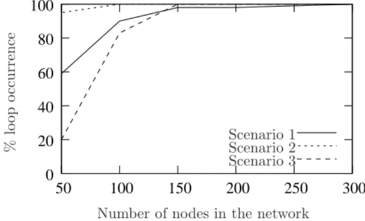
Figure 5 shows the percentage of loop occurrence as a function of the number of nodes in the network, for the three scenarios. In Scenario 1, the percentage of loop occurrence increases with the number of nodes. Even when the number of nodes is small (for instance, 50), the percentage of loop occurrence is about 60%, which means that loops are likely to occur. This comes from the fact that the two routing protocols build
paths with low correlations due to the random weight of R2. In Scenario 2, the percentage of loop occurrence
is about 100% for all numbers of nodes in the network. This is due to the fact that R1 and R2 yield to
different routing decisions, thus paths have a very low correlation. In Scenario 3, the percentage of loops
is low for a small number of nodes. Indeed, since the link metrics are correlated, R1 and R2 are likely to
be similar, so packets are likely to follow similar paths. However, when the number of nodes is large, the two routing protocols exhibit differences, and the resulting shortest paths have low correlations (even if the weights are correlated).
0 20 40 60 80 100 50 100 150 200 250 300
Number of nodes in the network
% lo o p o cc u rr en ce Scenario 1 Scenario 2 Scenario 3
Figure 5: In random networks, when R1is based on a hop-count metric and R2is based on a random metric, the percentage of
loop occurrence is high, due to the low correlation of the metrics of R1and R2. When R1and R2are both based on a random
metric, the percentage of loop occurrence is very high, again due to the very low correlation of the metrics of R1and R2. When
R1is based on a random metric and R2is based on a deviation of the metric of R1, the percentage of loop occurrence is high
for topologies with a large number of nodes, despite the high correlation of the metrics.
4.2.2. Loop occurrences on real networks
In this subsubsection, we quantify the number of loops that might appear using R1 and R2, for real
networks.
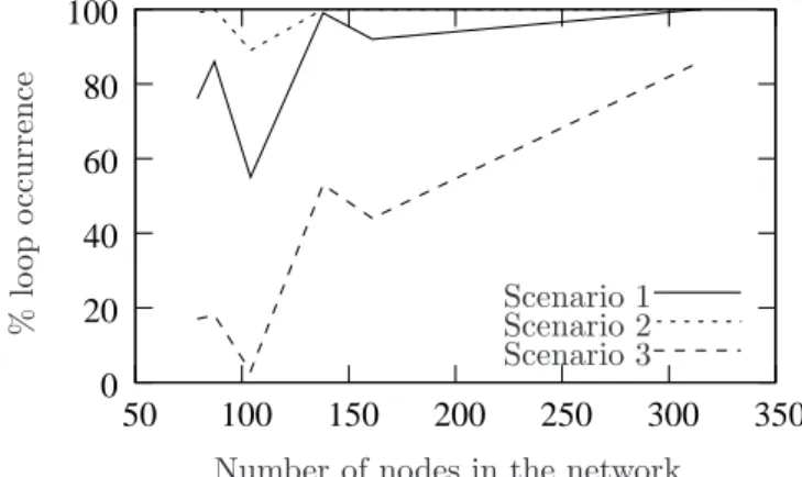
Figure 6 shows the percentage of loop occurrence as a function of the number of nodes, for the three scenarios. We notice that the percentage of loop occurrence is much larger with Scenario 1 and Scenario 2
than with Scenario 3. This is due to the fact that the routing protocols R1 and R2of Scenario 3 are highly
correlated. However, the percentage of loop occurrence is more important for large networks as the paths are longer. For real networks, the percentage of loop occurrence depends on the underlying topology. In general, this percentage increases with the network size, but there are some real topologies (such as the Rocketfuel topology ’1221.city’ with 104 nodes) that yield few routing loops (see also Figure 16 of [8]).
0 20 40 60 80 100 50 100 150 200 250 300 350
Number of nodes in the network
% lo o p o cc u rr en ce Scenario 1 Scenario 2 Scenario 3
Figure 6: In real networks, for Scenario 1, the percentage of loops is high (between 50% and 80% for small networks (less than 104 nodes), and above 90% for large networks). For Scenario 2, the percentage of loops is always high independently of the network size (between 90% and 100%). For Scenario 3, the percentage of loops increases with the network size (10% for small networks and up to 90% for large networks).
4.3. Average percentage of troublesome destinations
In this subsection, we focus on the percentage of troublesome destinations. Troublesome destinations are destinations that require to be considered independently by RTH and RTH-p. These destinations cannot follow the common per-router ordering used for all the remaining destinations.
We compute the number of troublesome destinations for random and real networks by averaging over 100 simulations, and we normalize it with respect to the number of nodes of the network in order to obtain a percentage. All nodes act as destinations.
4.3.1. Troublesome destinations for random networks
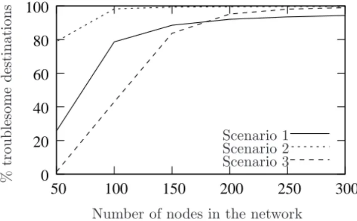
Figure 7 shows the average percentage of troublesome destinations in random networks. We notice that the percentage of troublesome destinations is low for small networks and increases consistently for large networks. This is due to the fact that the percentage of loop occurrence is small (cf Subsubsection 4.2.1). Moreover, the percentage of troublesome destinations depends on the scenarios. In Scenario 1, we notice that the percentage of troublesome destinations is low for small networks (less than 26%) but it increases quickly for large networks (up to 94%). In Scenario 2, the percentage of troublesome destinations is about 80% for a network of 50 nodes and goes up to about 100% for a network of 300 nodes. In Scenario 3, the percentage
of troublesome destinations is almost zero for small networks when R1 and R2 are highly correlated, but it
increases up to 98% for large networks.
4.3.2. Troublesome destinations for real networks
Figure 8 shows the percentage of troublesome destinations in real networks. For Scenario 1 and Scenario 2, the percentage of troublesome destinations is important (between 70% and 100% for Scenario 1, and above 90% for Scenario 2) for large networks. This percentage is low for small networks as paths to destinations are smaller, which leads to a small number of loops in the network (cf Subsubsection 4.2.2). For Scenario 3, the percentage of troublesome destinations is low, even for large networks. Note that the low percentage of troublesome destinations for Scenario 3 is the main argument used by authors of [8] to justify that there are few troublesome destinations. However, we believe that Scenario 3 represents only a specific case, where the two routing protocols are highly correlated.
0 20 40 60 80 100 50 100 150 200 250 300
Number of nodes in the network
% tr o u b le so m e d es tin a tio n s Scenario 1 Scenario 2 Scenario 3
Figure 7: In random networks, the percentage of troublesome destinations is more important in large networks than in small networks. Troublesome destinations appear even with correlated routing protocols (such as in Scenario 3).
0 20 40 60 80 100 50 100 150 200 250 300 350
Number of nodes in the network
% tr o u b le so m e d es tin a tio n s Scenario 1 Scenario 2 Scenario 3
Figure 8: In real networks, the percentage of troublesome destinations is more important in large networks than in small networks. Correlated routing protocols (see Scenario 3) are able to greatly reduce the number of troublesome destinations.
4.4. Results on average number of steps
In this subsection, we evaluate the number of steps required for all the nodes to change from R1 to R2
without any loop occurrence. This is our main metric, as the change duration is proportional to the number of steps produced by the heuristics.
We consider that all nodes are destinations. Simulation results are averaged over 100 repetitions and confidence intervals of 95% are shown.
We compare our heuristic SCH-p to RTH [8]. Recall that RTH provides an ordering to change the nodes sequentially: the number of steps of RTH is equal to the number of nodes in the network, if there is no troublesome destination. We also compare our heuristic SCH-p to RTH-p. Recall that RTH-p consists of changing several nodes in parallel.
4.4.1. Number of steps for random networks
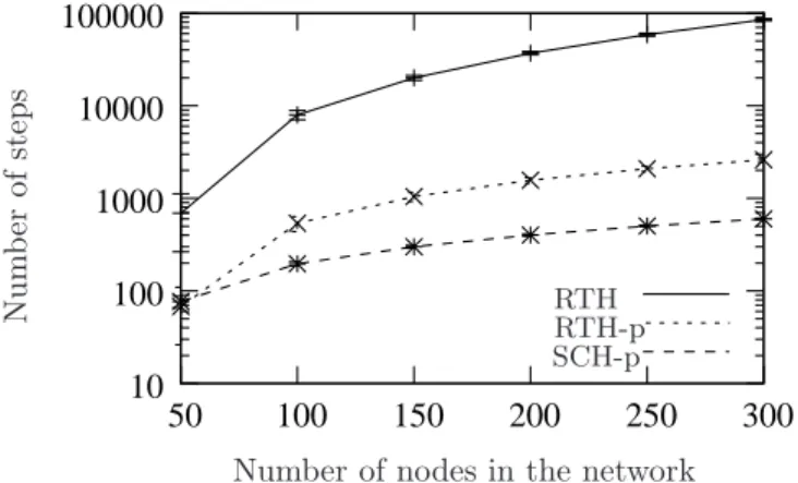
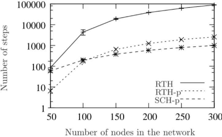
Figure 9 shows the average number of steps required to change the routing protocol, in term of the number of nodes in the network, for Scenario 1. The y-axis is depicted using a logarithmic scale. We notice that the number of step increases consistently with the size of the network for all the heuristics (RTH, RTH-p and SCH-p). We notice also that the number of steps is very large for RTH. This is due to the fact that only
one node at each step is able to change from R1to R2. More precisely, the number of steps for RTH is equal
to the number of nodes in the network, times α + 1, where α is the number of troublesome destinations. Both RTH-p and SCH-p outperform RTH with a gain that reaches up to 97% for RTH-p, and up to 99% for SCH-p. SCH-p outperforms RTH-p: for large networks (more than 100 nodes), SCH-p shows a gain of 63% for a network of 100 nodes, and a gain of 77% for a network of 300 nodes. The large gain of SCH-p can be explained as follows:
• SCH-p is able to change the routing protocol of nodes independently on their position on the paths
from the sources to the destinations (according to R2), while RTH-p only changes the routing protocol
for nodes starting from the destinations and going backward to the sources.
• Since the number of troublesome destinations is large (see Fig. 7), RTH-p is not able to aggregate many non-troublesome destinations together.
10 100 1000 10000 100000 50 100 150 200 250 300
Number of nodes in the network
N u m b er o f st ep s RTH RTH-p SCH-p
Figure 9: In random networks for Scenario 1, SCH-p is able to perform the change in about 600 steps on average for large networks. RTH and RTH-p require respectively 85182 steps and 2602 steps to perform the change of all the nodes.
Figure 10 shows the average number of steps required to change the routing protocols in term of the number of nodes, for Scenario 2. The y-axis is depicted using a logarithmic scale. We can see that the number of steps increases consistently with the size of the network. We notice also the same behavior for RTH as in Fig. 9: the number of steps required to change all the nodes is very large, especially for large networks. RTH produces 2021 steps for networks of 50 nodes, and 90000 steps for networks of 300 nodes.
10 100 1000 10000 100000 50 100 150 200 250 300
Number of nodes in the network
N u m b er o f st ep s RTH RTH-p SCH-p
Figure 10: In random networks and for Scenario 2, SCH-p is able to perform the change in about 761 steps on average for large networks. RTH and RTH-p require respectively 90000 steps and 3864 steps to perform the change of all the nodes.
SCH-p outperforms RTH-p (respectively RTH), with a gain varying from 57% (respectively 94%) for small networks up to 80% (respectively 99%) for large networks.
Figure 11 shows the average number of steps in term of the number of nodes in the network, for Scenario 3. The y-axis is depicted using a logarithmic scale. RTH-p shows a better behavior than SCH-p for small networks of less than 150 nodes. Indeed, RTH-p shows a gain of 89% for a network of 50 nodes and 11% for a network of 100 nodes compared to SCH-p. Those gains are due to the fact that there are few troublesome
destinations in this case, as R1 and R2 are highly correlated. Recall that SCH-p considers destinations
independently, and thus is not able to benefit from non-troublesome destinations. SCH-p is better than RTH-p for large networks. Indeed, SCH-p shows a gain of 42% for a network of 150 nodes and of 61% for a network of 300 nodes, compared to RTH-p.
1 10 100 1000 10000 100000 50 100 150 200 250 300
Number of nodes in the network
N u m b er o f st ep s RTH RTH-p SCH-p
Figure 11: In random networks and for Scenario 3, SCH-p is able to perform the change in about 998 steps on average for large networks. RTH and RTH-p require respectively 89361 steps and 2585 steps to perform the change of all the nodes.
4.4.2. Number of steps for real networks
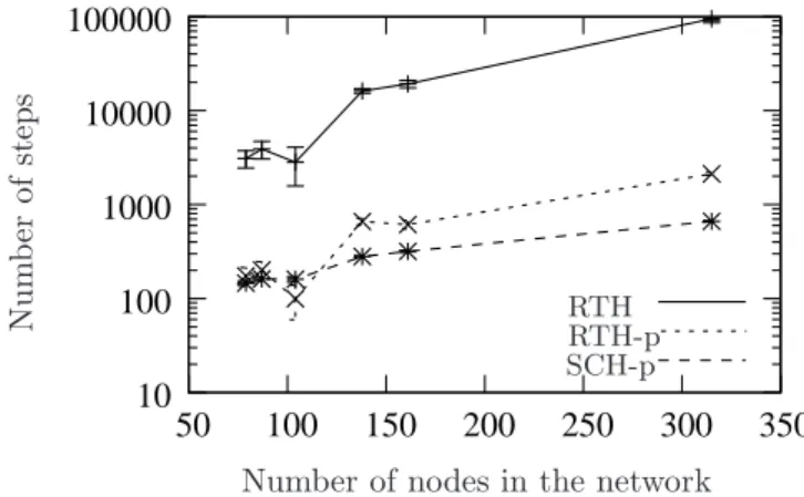
Figure 12 shows the average number of steps in term of the number of nodes for Scenario 1 and Rocketfuel topologies. The y-axis is depicted using a logarithmic scale. We notice the same behavior as for random networks. For small networks, SCH-p and RTH-p achieve a similar performance. For large networks, SCH-p shows better performance than RTH-p: SCH-p shows a gain that reaches 99% compared to RTH and 68% compared to RTH-p, for a network of 315 nodes.
Figure 13 shows the average number of steps in term of the number of nodes in the network, for Scenario 2, using a logarithmic scale. The gain of SCH-p reaches 96% for the smallest network compared to RTH, and
10 100 1000 10000 100000 50 100 150 200 250 300 350
Number of nodes in the network
N u m b er o f st ep s RTH RTH-p SCH-p
Figure 12: In real networks and for Scenario 1, SCH-p is able to perform the change in about 664 steps on average for the largest network (315 nodes). RTH and RTH-p require respectively 94890 steps and 2121 steps to perform the change of all the nodes.
48% compared to RTH-p. The largest gain reached for the largest network is 99% compared to RTH, and 69% compared to RTH-p. 100 1000 10000 100000 50 100 150 200 250 300 350
Number of nodes in the network
N u m b er o f st ep s RTH RTH-p SCH-p
Figure 13: In real networks and for Scenario 2, SCH-p is able to perform the change in about 869 steps on average for the largest network. RTH and RTH-p require respectively 99102 steps and 2851 steps to perform the change of all the nodes.
Figure 14 shows the average number of steps in term of the number of nodes in the network, for Scenario 3, using a logarithmic scale. RTH-p is better than SCH-p due to the very small number of troublesome destinations in this specific scenario and for these specific networks. The gain of RTH-p reaches 94% for a network of 104 nodes.
The computation time of SCH-p is larger than the computation time of RTH and RTH-p. With our mono-thread implementation on a i7-2600 CPU at 3.40 GHz (with eight cores), SCH-p is able to compute all the steps for the largest real topology in 91 seconds on average (with a standard deviation of 3 seconds, and for Scenario 2 which yields the largest number of loops). RTH and RTH-p compute all the steps in 1.5 seconds and 2.2 seconds respectively. However, we believe that the computation time of SCH-p is reasonable for large networks of 300 nodes, and that the gain of the change duration outweights the computation time. 5. Conclusion
When a routing protocol has to be changed, transient routing loops might occur in the network. In this paper, we quantified the percentage of loop occurrence on several scenarios. We show that loops can be completely avoided by having nodes change their routing protocol according to a sequence which depends
1 10 100 1000 10000 100000 50 100 150 200 250 300 350
Number of nodes in the network
N u m b er o f st ep s RTH RTH-p SCH-p
Figure 14: In real networks and for Scenario 3, RTH-p is generally better than SCH-p due to the very low number of troublesome destinations. SCH-p performs the change in about 666 steps for the largest network. RTH and RTH-p require respectively 59629 steps and 698 steps to perform the change of all the nodes.
on the topology and on the routing protocols. This sequence is a list of steps, where each step is a set of nodes that can change their routing protocol in arbitrary order. We proposed RTH-p, an enhancement of the RTH heuristic [8], that is able to change several nodes in parallel. Then, we proposed SCH-p, a centralized heuristic which builds sequences with a small number of steps. Reducing the number of steps is crucial, as the duration of a change is proportional to the number of steps. Simulation results for random and real networks show that SCH-p outperforms both RTH and RTH-p in most scenarios. The gain of SCH-p in term of number of steps varies between 80% and 99% when compared to RTH, and between 61% and 77% for most large networks when compared to RTH-p.
References
[1] K. Butler, T. R. Farley, P. McDaniel, J. Rexford, A survey of BGP security issues and solutions, Proceedings of the IEEE 98 (1) (2010) 100–122.
[2] P. Trakadas, T. Zahariadis, S. Voliotis, P. Karkazis, T. Velivassaki, L. Sarakis, Routing metric selection and design for multi-purpose WSN, in: IWSSIP (International Conference on Systems, Signals and Image Processing), 2014, pp. 199–202.
[3] Z. Zhong, R. Keralapura, S. Nelakuditi, Y. Yu, J. Wang, C. N. Chuah, S. Lee, Avoiding transient loops through interface-specific forwarding, in: IEEE/ACM IWQoS (International Symposium on Quality of Service), Vol. 3552 of Lecture Notes in Computer Science, Springer, 2005, pp. 219–232.
[4] P. Francois, O. Bonaventure, Avoiding transient loops during the convergence of link-state routing proto-cols, IEEE/ACM Transactions on Networking 15 (6) (2007) 1280–1292. doi:10.1109/TNET.2007.902686. [5] S. Nelakuditi, Z. Zhong, J. Wang, R. Keralapura, C. N. Chuah, Mitigating transient loops through
interface-specific forwarding, Computer Networks 52 (3) (2008) 593–609.
[6] N. El Rachkidy, A. Guitton, M. Misson, Avoiding routing loops in a multi-stack WSN, JCM (Journal of Communications) 8 (3) (2013) 751–761.
[7] N. El Rachkidy, A. Guitton, M. Misson, Improving routing performance when several routing protocols are used sequentially in a WSN, in: ICC (IEEE International Conference on Communications), 2013, pp. 1408–1413.
[8] L. Vanbever, S. Vissichio, C. Pelsser, P. Francois, O. Bonaventure, Lossless migrations of link-state IGPs, IEEE/ACM Transactions on Networking 20 (6) (2012) 1842–1855.
[9] R. Shirani, M. St-Hilaire, T. Kunz, Y. Zhou, J. Li, L. Lamont, Combined reactive-geographic routing for unmanned aeronautical adhoc networks, in: IWCMC (International Wireless Communications and Mobile Computing Conference), 2012.
[10] S. Moad, M. T. Hansen, R. Jurdak, B. Kusy, N. Bouabdallah, A. Ksentini, On balancing between minimum energy and minimum delay with radio diversity for wireless sensor networks, in: IFIP Wireless Days, 2012.
[11] M. Fonoage, M. Cardei, A. Ambrose, A QoS based routing protocol for wireless sensor networks, in: IPCCC (IEEE Performance Computing and Communications Conference), 2010.
[12] J. Steffan, L. Fiege, M. Cilia, A. P. Buchmann, Towards multi-purpose wireless sensor networks, in: Systems Communications, 2005, pp. 336–341.
[13] J. Steffan, M. Voss, Security mechanisms for multi-purpose sensor networks, in: GI Jahrestagung, Vol. 2, 2005, pp. 158–160.
[14] D. Manjunath, S. V. Gopaliah, A multi-purpose wireless sensor network for residential layouts, in: BWCCA (International Conference on Broadband and Wireless Computing, Communication and Ap-plications), 2007, pp. 49–58.
[15] P. Javier del Cid, Optimizing resource use in multi-purpose WSNs, in: PerCom Workshops (Pervasive Computing Workshops), 2011, pp. 395–396.
[16] L. Sarakis, T. Zahariadis, H.-C. Leligou, M. Dohler, A framework for service provisioning in virtual sensor networks, EURASIP Journal on Wireless Communications and Networking (1) (2012) 135. [17] F. Clad, P. Merindol, J.-J. Pansiot, P. Francois, O. Bonaventure, Graceful convergence in link-state IP
networks: A lightweight algorithm ensuring minimal operational impact, IEEE/ACM Transactions on Networking 22 (1) (2013) 300–312. doi:10.1109/TNET.2013.2255891.
[18] F. Clad, P. Merindol, S. Vissicchio, J.-J. Pansiot, P. Fran¸cois, Graceful router updates for link-state protocols, in: IEEE ICNP (International Conference on Network Protocols), 2013.
[19] R. E. Tarjan, Depth-first search and linear graph algorithms, SIAM Journal on Computing 1 (2) (1972) 146–160.
[20] N. Spring, R. Mahajan, D. Wetherall, Measuring ISP topologies with rocketfuel, in: ACM SIGCOMM, 2002, pp. 133–145.